Article

An Optimal Control Method for Greenhouse Climate Management Considering Crop Growth’s Spatial Distribution and Energy Consumption

School of Electrical and Information Engineering, Jiangsu University, Zhenjiang 212013, China
*
Author to whom correspondence should be addressed.
Energies 2023, 16(9), 3925; https://doi.org/10.3390/en16093925
Submission received: 20 March 2023 / Revised: 28 April 2023 / Accepted: 3 May 2023 / Published: 6 May 2023

Abstract

:
The environmental factors of greenhouses affect crop growth greatly and are mutually coupled and spatially distributed. Due to the complexity of greenhouse climate modeling, the current optimal control of greenhouse crop growth rarely considers the spatial distribution issues of environmental parameters. Proper Orthogonal Decomposition (POD) is a technique to reduce the order of a model by projecting it onto an orthogonal basis. In this paper, POD is used to extract environmental features from Computational Fluid Dynamics (CFD) simulations, and a low-dimensional feature subspace is obtained by energy truncation. With multi-dimensional interpolation, fast and low-dimensional reconstruction of the dynamic variation of greenhouse climates is achieved. On this basis, a rolling-horizon optimal control scheme is proposed. For each finite horizon, the external meteorological data are updated, and the response of the greenhouse environment is quickly calculated by the POD model. With the performance criterion J of maximizing crop production and energy efficiency, through the particle swarm optimization algorithm, the optimal settings for the greenhouse shading rate and the fan speed are derived. Such control computations are rolled forward during the whole planting season. Results of a case study show that the proposed method has low computation cost and high spacial resolution and can effectively improve the spatiotemporal accuracy of greenhouse climate management. In addition, different from traditional global optimal control methods, the proposed rolling-horizon scheme can correct various external disturbances in the procedure of crop growth, and thus it is more robust and has potential for engineering applications.

1. Introduction

With the growing population, depletion of resources and regional conflicts, it becomes gradually important to increase food production and energy consumption efficiency [1]. Greenhouse planting can overcome unfavorable conditions of outdoor climate and geography and thus plays a significant role in modern agriculture, especially in densely populated areas in China. As a complex, high-dimensional system, the process of greenhouse climate variation contains mutually interacting sub-processes with large differences in response times and spaces. With the development of computing power and artificial intelligence, practical designs of greenhouse climate management to promote crop growth and save energy usage have attracted more and more attention [2,3,4,5]. The main idea of such control techniques relies on using an objective function based on climatic and crop models over different timescales to determine the optimal trajectories of the main environmental variables. For example, Van Henten proposed a receding-horizon optimal control strategy to derive the main environmental variable trajectories throughout lettuce production [6,7]. To handle time-varying parameters of the greenhouse crop model, Xu et al. [8] applied a two-time-scale optimal controller for greenhouse crop cultivation with online parameter estimation. Similar studies can be found in [4,5,9,10,11]. However, for large greenhouses, the distribution of environmental parameters in the crop area is not uniform. The environmental variables to which the crops are subjected are not equivalent to the control outputs of the actuators at the greenhouse boundary. To this end, without considering the spatial distribution of the greenhouse, the environmental control sequence derived from the above studies is not strictly optimal, but it is sub-optimal. Limited by the computational cost of environmental simulation, there are few solutions to this problem.
A greenhouse system contains multiple mutually interacting subsystems such as the indoor climate, crop dynamics (photosynthesis, respiration and transpiration) and crop growth. Although there are several engineering practices for indoor environment modeling, including nodal methods, zone methods, etc., Most of them only follow the laws of energy conservation and mass conservation and do not meet the requirements of greenhouse planting systems. Relatively, CFD methods are a suitable option. In fact, CFD simulation has been widely used for high-resolution modeling and analysis of greenhouse flow fields. For example, Santorini et al. [12] used a CFD method to study the numerical characteristics of natural ventilation in a greenhouse. Zhang et al. [13] conducted CFD analysis on the spatial distribution of the  CO 2  concentration in a strawberry greenhouse. Kim et al. [14] used three-dimensional CFD to study the humidity distribution in a greenhouse that was validated by experimental data. It is noted that due to the complex modeling and high computational cost, CFD methods are mostly oriented towards systems analysis, not optimal control [15]. Combining CFD simulation with model reduction tools to build a low-dimensional surrogate model of a greenhouse environment is a new perspective. In 2008 and 2013, Sempey et al. [16] and Li et al. [17], respectively, successfully rebuilt indoor dynamical temperature fields based on POD order reduction. Similar studies include [18,19,20,21,22]. In 2020, Li et al. [23] first introduced the POD method to the greenhouse production field. Reduced-order models of the temperature field and carbon dioxide concentration distribution in a greenhouse were reconstructed. By combining a spline interpolation tool with the obtained low-dimensional parameter models, the greenhouse environmental response can be solved fast with low computation cost. It is interesting to combine low-dimensional environmental models with climate-optimal control strategies. This will help us understand the spatial distribution of crop growth trends, which will guide us to adjust the greenhouse climate to optimal conditions with high spatial resolution. The challenges are: (1) During the whole crop growth cycle, the external meteorological data changes a lot and external disturbances exist. How do we quickly solve the greenhouse environmental response with high-resolution at each time step? (2) The greenhouse climate model is built by a CFD-POD method, and crop growth is commonly modeled by differential equations. How do we coordinate the parameters of two such different types of models? (3) From the engineering sense, the external meteorological conditions for the entire crop growth cycle are not known in advance. How do we design a finite-horizon optimal control method based on short-term weather data?
In view of the above issues, this paper aims to propose a rolling-horizon optimal control strategy considering crop growth spatial distribution. The main contributions of this paper are as follows:
(1)
A reduced-dimensional model of the greenhouse climate is rebuilt by the POD method and can provide indoor climate variation with high spatial resolution. With different external meteorological data, the response of the greenhouse environment can be quickly solved by multi-dimensional interpolation for each control step.
(2)
The low-dimensional model of the greenhouse climate is integrated with a simplified crop growth model. The environmental values to which the crop is subjected are coordinated with the ambient parameters of the crop area in the climate model.
(3)
Considering that the external meteorological conditions are not known in advance for the entire planting season, a finite-horizon optimal control strategy is proposed. The control horizon is set based on external weather condition forecasting. At each finite horizon, the PSO optimization algorithm is applied to adjust the control variables of the climate model. Such control action rolls forward during the whole crop growth cycle.
(4)
Through a case study, the effects of this method on economic benefits and energy saving are validated and analyzed.
The rest of this paper is organized as follows: Section 2 describes basic principles and methods used in this study, including the reduced-dimensional modeling method, the greenhouse crop modeling method and the whole optimal control scheme. Section 3 presents the construction procedure of the proposed greenhouse climate model. Section 4 carries out a case study using the proposed optimal control scheme. Section 5 provides a brief discussion of this method. The Conclusion Section gives some remarks and future work.

2. Method

2.1. Reduced-Dimensional Modeling of Greenhouse Climate

2.1.1. Principles of POD Method

Proper orthogonal decomposition can be regarded as the optimal linear reconstruction model in the sense of the least squares [24]. POD has been widely used to reduce the dimensions of distributed environmental data [18,19,20]. After POD order reduction, by an interpolation operation within the obtained low-dimensional parameter sub-space, the response of the greenhouse climate can be solved quickly without losing the features of the original model.
The basic idea of POD is: given a data set  θ k H k = 1 n  in the n-dimensional vector space V, find a group of m-dimensional ( m < < n ) subsets s to form a subspace, minimizing the error  E θ k P s θ k  in mapping the original data to the subset, where V is assumed to be a Hilbert space with inner product  · , · θ k P s θ k  is the energy norm of H, and  P S  is the orthogonal mapping of the subspace S. In the application of greenhouse climate modeling, the dimension of the  θ k  vector represents the grid number of the area of interest [25]. The above problem can be transformed to an eigenvalue problem, where R is a square matrix of order n:
R = E x k x k * ,
R φ k = λ k φ k , λ 1 λ n 0 ,
where  φ K  is the eigenvector, or the so-called POD mode.
In the CFD simulation, the dimension of n is huge, which results in the very high calculation cost of R. To this end, the snapshot solution method is applied in practice [23]. The snapshot solution method selects m groups of linearly independent data in the n-dimensional vector space V and uses the linear combination of these m groups of data to replace  φ K ; it can be formulated as:
φ K = k = 1 m C k θ k .
By combining Equations (1)–(3), we get
E x k x k * × k = 1 m C k θ k = λ k = 1 m C k θ k .
According to the property of tensor products, the above equation can be simplified as
1 m A T A C = λ C ,
where A is the original data matrix obtained by CFD simulation, and  A T A  is an m-order square matrix. Because  m < < n , the calculation is simplified effectively.

2.1.2. Reduced-Dimensional Modeling of Greenhouse Climate

The above POD method has achieved satisfactory results in the dynamic/steady-state simulations of indoor environments [16,17]. From a mathematical point of view, the POD method in an agricultural greenhouse climate system is used to find and extract the dominant eigenvectors of environmental factors through multiple snapshots within the feasible range of the control variables. Through the linear combination of mode coefficients and eigenvectors, the subspace of environmental factor variation is reconstructed quickly. In this way, calculation of the greenhouse environmental response is transformed from complex CFD simulations to the interpolation of the mode coefficients. Such a modeling procedure consists of two offline–online stages, which will be specified in Section 2.3.
The reconstruction of a low-dimensional environmental model based on POD mainly includes the following steps:
S1.
Set up a proper CFD model of the greenhouse climate considering external meteorological data and crop dynamics.
S2.
Determine control variables and their feasible ranges. Set the variation range of external weather conditions.
S3.
Fully sample within the multi-dimensional space composed of the above control variables and external environmental parameters and carry out CFD steady simulations accordingly.
S4.
Extract the response parameter fields of each simulation (snapshots).
S5.
Reconstruct parameter variation subspaces by POD (see Section 2.1(1) for details).
S6.
According to the actual changes to the control variables/external conditions, apply multiple-dimensional interpolation in the obtained parameter subspace for fast acquisition of the greenhouse climate response.

2.2. Greenhouse Crop Growth Modeling

A greenhouse system has complex, mutually interacting processes between the indoor climate and crop growth. On the basis of the greenhouse climate model, a simplified lettuce growth process is modeled in this study. It is known that Henten’s four-state-variable dynamic model [9] integrates a one-state-variable lettuce growth model (including one state variable: crop dry weight) and a greenhouse climate model (including three state variables: air temperature, air humidity and carbon dioxide concentration). The adequacy of this model has been verified based on the destructive measurement of 20 plants at multiple sample dates [7]. A similar verification can be found at [26]. In this study, the greenhouse crop model refers to the basic principles of Henten’s model. The difference is that the climate-related state variables are either directly extracted from the POD climate model or are simplified according to the planting conditions. The lettuce growth model refers to Henten’s equation with crop dry matter as the main state variable. The first-difference form of the model is as follows:
X d ( i + 1 , k ) = C α β φ p h o t ( i , k ) C r e s p X d ( i , k ) × 2 0.1 X T ( i , k ) 2.5 + X d ( i , k ) φ p h o t ( i , k ) = 1 e C p l , d X d ( i , k ) × C r a d , p h o t V r a d ( C c o 2 , 1 X T ( i , k ) 2 + C c o 2 , 2 X T ( i , k ) C c o 2 , 3 ) ( X c C Γ ) C r a d , p h o t V r a d + ( C c o 2 , 1 X T ( i , k ) 2 + C c o 2 , 2 X T ( i , k ) C c o 2 , 3 ) ( X c C Γ ) ,
where  C α β  is the yield factor,  φ p h o t  is the photosynthetic rate,  C r e s p  is the respiratory rate,  C p l , d  is the effective canopy surface,  C r a d , p h o t  is the light utilization efficiency, and  V r a d  is the solar radiation outside the greenhouse;  C c o 2 , 1 C c o 2 , 2  and  C c o 2 , 3  describe the effect of temperature on the total photosynthesis of the canopy,  X c  is the state variable of carbon dioxide concentration, and  C Γ  represents the carbon dioxide compensation point. The values of related coefficients also refer to Henten’s report [7,9] (Table 1).
From the above lettuce model, it is seen that the crop dry weight  X d  is mainly determined by the indoor air temperature  X T , the solar radiation  V r a d  and the carbon dioxide concentration  X c . For this study, the indoor air temperature  X T  is extended to  X T ( i , k ) , and its value is extracted from the greenhouse climate model, which can derive air temperature at each time step and grid cell (i represents the time step and k means the  N o .  of the grid cell). The value of solar radiation  V r a d  is calculated by an external meteorological report and the shading rate of the greenhouse. Considering the planting conditions of East China’s summer, the carbon dioxide concentration  X c  is not set as a control variable and is simplified to a constant equal to the atmospheric concentration. The photosynthesis and respiration of crops are directly given by Equation (6) [7].

2.3. The Optimal Control Scheme

2.3.1. Statement of the Climate-Optimal Control Problem

Different from other greenhouse climate models, the environmental factors affecting crop growth are simulated by two models in this study. The crop growth model simulates the increase in dry weight that is mainly affected by ambient air temperature, solar radiation and carbon dioxide concentration (as a constant). In the greenhouse climate model, porous material is used to simulate the crop area. According to the description in Section 2.2, the coordination of the two models occurs mainly at the temperature field of the crop area. The temperature distribution of the crop canopy is solved by CFD simulation considering various environmental factors’ influences (outdoor radiation, outdoor air temperature, relative humidity and air speed). The resulting values of the temperature field at time step k are transferred to  X T ( i , k )  of the crop growth model. In this way, the reduced greenhouse climate model and lettuce growth equations are integrated to generate numerical solutions to the optimal control problem.
The control variables are set according to field conditions of the greenhouse. In this study, they are the ceiling shading rate and the fan speed of the greenhouse. The control variables both have equality constraints, which will be specified in the following section.
From the engineering sense, the external meteorological conditions cannot be predicted accurately in advance for the entire planting season. To this end, a kind of finite-horizon optimal control strategy is proposed that is more feasible than global optimal control methods. Based on the outdoor weather’s prediction time domain, the control horizon is set accordingly. Step by step, the control action rolls forward during the whole crop growth cycle. It should be noted that unlike traditional global optimal controls, rolling optimal control cannot obtain the ideal global optimal solutions because the performance criteria are set piecewise for finite horizons. However, considering the complexity of external weather variations, a finite-horizon optimal control strategy based on short-term weather prediction has better robustness, and the accuracy can be guaranteed.
Crop yield and energy efficiency during the planting process are the two main targets for greenhouse climate management. The crop dry matter weight is linearly related to the crop yield. For each control time horizon, the dry matter increase is converted to economic benefit, and the energy usage is converted to economic cost. Thus, for finite horizon  [ T 0 , T s ] , the performance criteria is set as following:
m a x J = Φ X d ¯ ( i ) L v f a n ( i ) Φ X d ¯ ( i ) = C λ , 1 1 C λ , 2 S g h C p r i c e , 1 × i = T 0 T s X d ¯ ( i ) L v f a n ( i ) = N f a n i = T 0 T s S f a n × v f a n ( i ) V f a n , r 3 P r C p r i c e , 2
where  Φ X d ¯ ( i )  is the converted economic benefit of crops for  [ T 0 , T s ] L ( v f a n ( i ) )  is the economic cost of electrical energy consumed by the greenhouse fan wet curtain system;  X d ¯ ( i )  is the average increase in the weight of crop dry matter in the crop area for one time step,  C λ , 1  is the ratio of wet weight to dry weight of lettuce,  C λ , 2  is the ratio of root dry weight of lettuce to total dry weight,  S g h  is the crop area, and  C p r i c e , 1  is the price of lettuce in the wholesale market;  S f a n  is the area of the greenhouse fan,  V f a n , r  is the rated air volume of the fan,  P r  is the rated power of the fan,  N f a n  is the number of fans, and  C p r i c e , 2  is the price of electricity per  kWh   [27].

2.3.2. PSO Optimization Algorithm

Since a CFD-based climate model is combined with a crop growth model for this optimal control issue, the traditional optimal control solutions are not applicable. In this study, searching for optimal solutions is carried out by a stochastic optimization algorithm—a particle swarm optimization algorithm—that has the characteristics of global search ability, a simple structure and fast search speed [28,29,30,31].
In the search space, composed of fan speed and shading rate for this paper, N particles are randomly placed with their positions and speeds initialized. For each iteration, the particle quality is evaluated by calculating the fitness value given by Equation (7). Note that the environmental response of the greenhouse for each particle is quickly calculated by POD. The position and speed of each particle is updated according to the individual’s best value (pbest) and the population’s best value (gbest). When the iteration number or accuracy requirements are met, the iteration stops and the optimal result is obtained. The details of the PSO algorithm can be found in [28].

2.3.3. Overall Optimal Control Framework Based on Offline–Online Strategy

Since the crop growth trend with high spatial resolution needs complex CFD simulations, the process of the overall optimal control framework is divided into two stages:
Offline stage: The CFD simulation of the greenhouse climate model is reduced by POD. The complex numerical iteration method of CFD is replaced by the fast interpolation method. Considering the outdoor meteorological data and the greenhouse structure, the greenhouse model is established and the control variables are set. Then, according to the ranges of main outdoor meteorological conditions and control variables, a sufficient number of sampling and corresponding steady simulations are conducted. The resulting temperature fields in the crop area are extracted, and POD is applied to rebuild a reduced-order temperature field variation space with respect to mode coefficients. In this way, the particles’ fitness function calculation can be accelerated by multiple-dimensional interpolation instead of CFD simulations.
Online stage: A simplified lettuce growth model is built in a first-order difference shape. According to the outdoor meteorological prediction timescale, the optimal control’s time horizon is set. The performance criteria considering economic benefits and energy savings is set. For each time horizon, the PSO algorithm is applied for optimal control variable searching in the control variable space. In each iteration of PSO, POD-based multiple-dimensional interpolation is carried out for greenhouse climate response calculation. The control operation rolls forward during the whole crop growth cycle. The overall optimal control framework is shown in Figure 1.

3. Construction of Greenhouse Climate Model

3.1. CFD Modeling

The greenhouse model used for optimal control in this paper refers to an actual greenhouse building located in Zhenjiang City, Jiangsu Province, China (longitude 119.452753 E, latitude 32.204402 N). The length of the greenhouse from north to south is 40 m, and the width from east to west is 18 m. The four walls and ceiling are made of float glass with light transmittance of 87%. Three negative-pressure fans are equipped in the north wall. In order to verify the stability and accuracy of the CFD model, the actual greenhouse is equipped with 36 wireless temperature sensors and 4 wind-speed sensors. The greenhouse’s location and structure are shown in Figure 2.
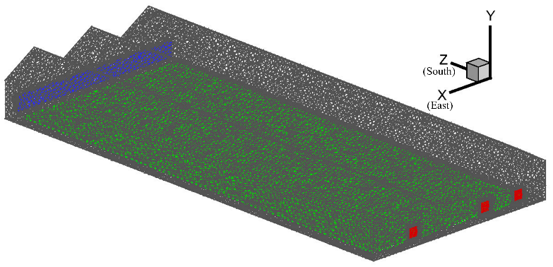
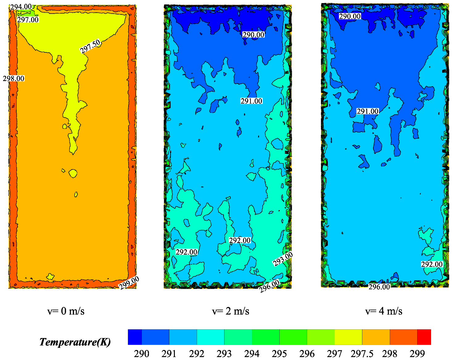
For CFD simulation, the fans are simplified to square holes with side lengths of 1 m. A wet curtain is simulated with a size of 38 m × 1.25 m and is located on the south wall 0.2 m above the ground. A cube is simulated as the crop area with a size of  l e n g t h × w i d t h × h e i g h t  = 36 m × 16 m × 0.2 m inside the greenhouse. The three-dimensional model is meshed with 72,492 grid units, and the wet curtain position is encrypted. The pressure-based solver is selected for model calculation. The standard  k ω  model is chosen for turbulence modeling. A discrete-coordinate DO model is used for radiation modeling. A porous material is used to simulate the crop area of the greenhouse. For simplicity, two momentum source terms, including viscous resistance terms and inertial resistance terms, are added to the momentum equation of the porous material, and the Ergun formula is used to estimate their values. To simulate the crop’s transpiration effect, a temperature boundary is set at the crop canopy. Referring to the data in other literature [32], the boundary temperature is simplified as a linear function of the wet curtain temperature and the external temperature. The geometric structure of the greenhouse model is shown in Figure 3, and the main physical properties of materials applied in the greenhouse model are listed in Table 2 [33,34]. Figure 4 provides the residual diagram of a typical CFD simulation by the above model setting, and Figure 5 provides the resulting temperature contours at three different fan speeds.

3.2. Reduced Model for Greenhouse Climate Variation

It is known that lettuce growth in greenhouses is sensitive to high temperatures. The most suitable temperature range for lettuce planting is  11 18 C . Ambient temperatures above  25 C  cause premature bolting, and temperatures above  28 C  cause slow growth and poor quality [35,36]. For greenhouses in summer in East China, the outdoor temperature and light intensity are usually higher than the proper values for lettuce growth. To this end, it is necessary to control the indoor temperature of the greenhouse to make it suitable for the growth of lettuce.
For summer planting, two months of hourly climate information for Zhenjiang City (Jiangsu Province, China) is collected from the US National Oceanic and Atmospheric Administration’s meteorological satellite (recorded in Figure 6).
According to the ranges of weather conditions collected, the variation ranges of the three main environmental parameters for the greenhouse are set as follows: the outside temperature range is  15 35 C , the outside humidity range is 35–100%, and the solar radiation range is 0–600 Wm 2 . Additionally, the feasible speed range of the wet curtain and the negative pressure fans is set to 0–4  ms 1 .
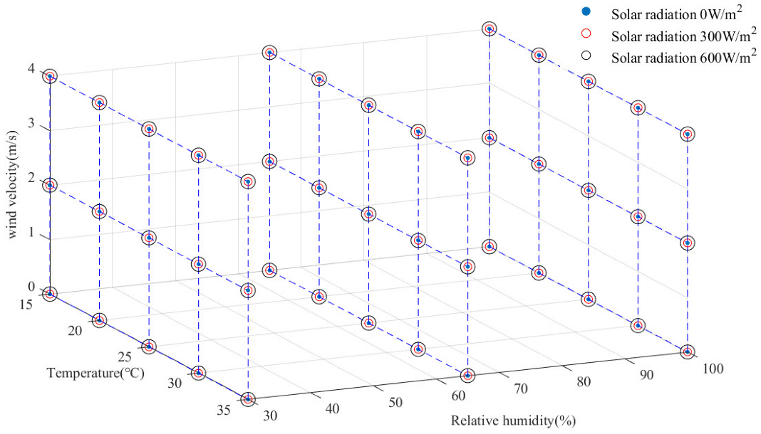
Within the four-dimensional space composed of these four main variables, 135 sample points are evenly sampled. Each sample point represents a parameter vector: [outside temperature, outside humidity, solar radiation, fan speed]. In this way, a total of 135 samples are evenly selected, as shown in Figure 7.
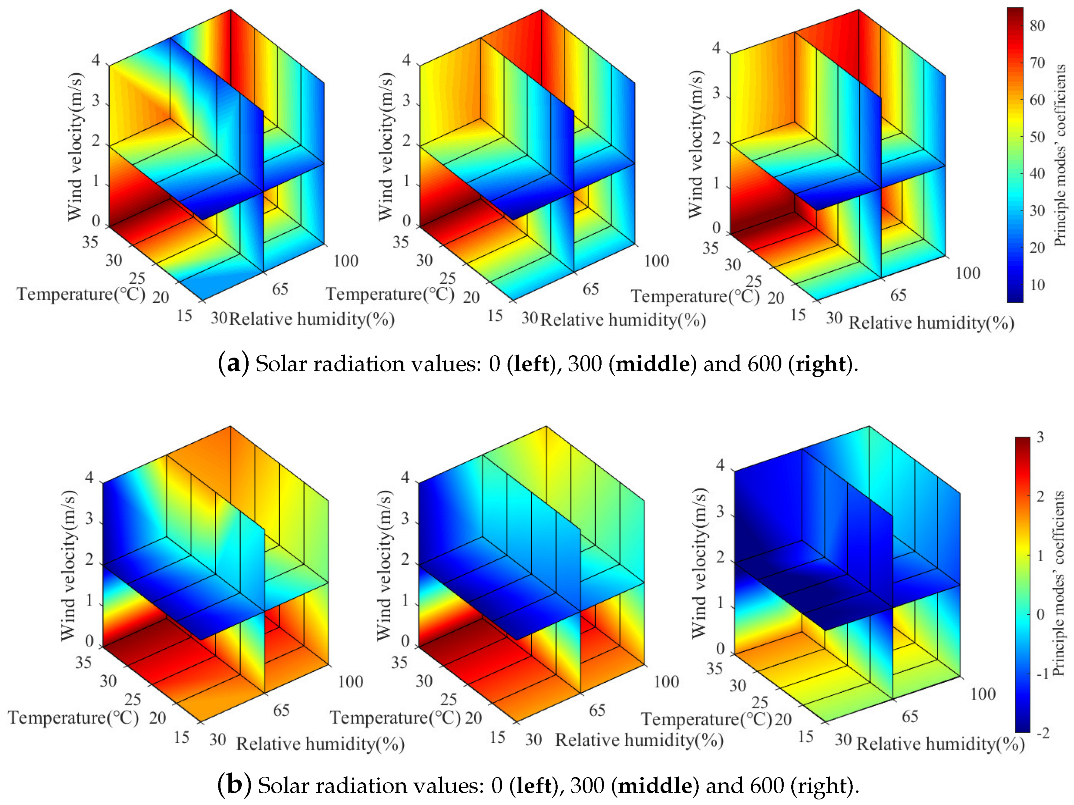
According to the selected parameter vector and other related boundary conditions, the corresponding 135 steady simulations of the greenhouse climate are performed during the offline stage. For POD order reduction, the temperature field, containing 8146 grids in the horizontal section 0.25 m above the ground, is extracted after each simulation. It represents the temperatures around the crop canopy, i.e.,  X T ( i , k )  in the crop growth equation (Equation (6)). The total of 135 temperature-field snapshots are straightened to form the temperature field variation matrix of the crop canopy, i.e., matrix A in Equation (5), whose dimensions are  8146 × 135 . According to the POD snapshot method mentioned in Section 2.1, the original eigenvalue problem is transformed into the eigenvalue problem of matrix  A T A , whose dimensions are  135 × 135 . By solving Equation (5), the eigenvalues  λ  and eigenvectors  Φ k  (POD modes) are solved. Thus, the temperature field’s variation (described by 135 snapshots) is transformed into a parameter subspace that can be described by the linear combination of POD modes and their coefficients. To ensure the obtained POD model contains more than 99% of the information of the original model, the first six energetic POD modes are retained [16]. Thus, when the actual weather condition is known (outside temperature, humidity and solar radiation), and the candidate control variables (fan speed and sunshade rate) from the optimal control iteration are set, the greenhouse climate response can be quickly solved by the interpolation of model coefficients within their distributions. Corresponding to the ranges of the four above variables, the distributions of the two most-principal mode coefficients are shown in Figure 8 as an example.
To verify the accuracy of the quickly obtained greenhouse climate response, experimental data from May 2017 [23] is compared with the temperature distribution from the POD model. The results show that the POD accuracy of the steady-state temperature field is consistent with that of experimental values, and the difference in temperature is no more than  0.8 C . More-detailed model validation can be found in our previous report [23]. Using the offline–online strategy, this method can obtain high-resolution greenhouse climate information quickly, which is the basis of the high-precision climate control described in the following section.

4. Optimal Control Results

4.1. Optimal Control Setting

For the purpose of optimal control with high spatial resolution, the reduced CFD model of the greenhouse climate and the simplified crop growth model are integrated as described in Section 2. From the engineering sense, the external meteorological data are assumed to come from short-term predictions (hourly). The finite-horizon optimal control strategy is applied for the optimal control of the greenhouse climate. The rolling-control horizon is set to one hour accordingly, and the whole planting cycle is set to 8 weeks. According to the actual planting conditions of the greenhouse, the control variables are set as ceiling shading rate and fan speed with equality constraints. The control target contains the maximum of dry weight increase and energy efficiency that is formulated in Equation (7). Because of the complexity of the mixed model, the stochastic optimization algorithm—the PSO algorithm—is used for optimal control variable searching in each control horizon. Considering the convergence efficiency, the particle number is set to 100 and the iteration number is set to 5. Although some parameters have been mentioned above, we summarize them together in Table 3.

4.2. Results and Analysis

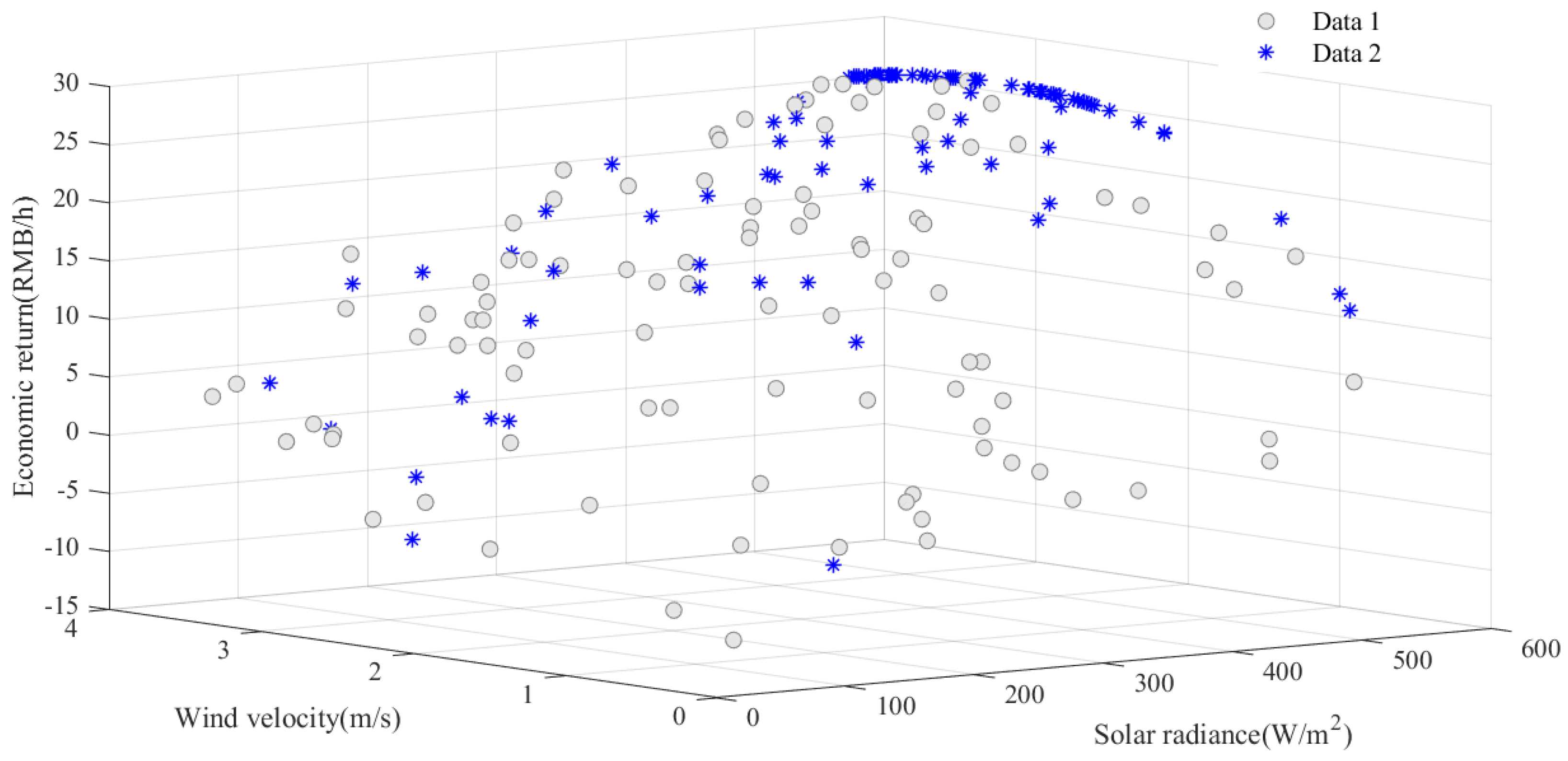
By using the mixed greenhouse model and parameter settings mentioned above, the proposed optimal control is conducted. To show the convergence efficiency of the PSO algorithm, a typical searching procedure for optimal control variables is recorded in Figure 9. It is seen that after five iterations, most of the particle swarm can converge to the optimal location successfully according to the fitness function.
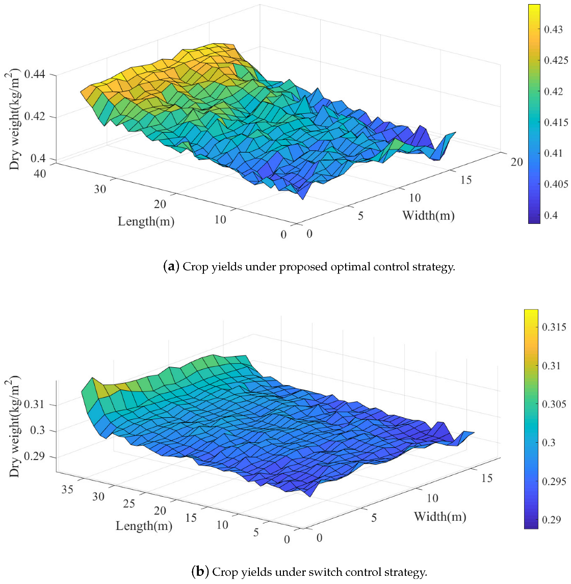
After the whole planting cycle of 8 weeks, the crop dry matter weight per square meter is derived and is shown in Figure 10a. From the figure, it is seen that due to the spatial inhomogeneity of greenhouse environmental parameters, the spatial distribution of the crop yield is different. By combining the POD-based reduced dimension greenhouse climate model with the crop growth model, the crop growth trend at each grid can be observed and controlled. In other words, the proposed method provides the ability to precisely manage the lettuce growth of the crop area in both temporal and spatial domains. From the result of the dry matter weight distribution, the crop weights near the wet curtain side are better than those near the other side. The two corner areas near the north wall have the lowest crop yield. The poor temperature regulation effect in these two zones may be the main reason. The corresponding control sequences of fan speed and sunshade rate during the whole planting cycle are recorded in Figure 11a and Figure 12, respectively.
To validate the effect of the proposed control strategy, another simple control scheme is also implemented for comparison. It belongs to a kind of switch control: that is, when the outdoor temperature is higher than  30 C , the fan speed is set to 4 m/s, and when the solar radiation is higher than 600 Wm 2 , the shading rate is set to  30 % . Figure 10b shows the crop dry matter weight per square meter under this switch control strategy. Compared with Figure 10a, it is obviously seen that crop yield under optimal control is much better than crop yield under switch control. The average weight of dry matter under optimal control is 0.43 kg/ m 2 , which is better than that under switch control (0.3 kg/m 2 ). Compared with the switch control method, the gross profit of the proposed method is increased by 42.75%. See Table 4 for a specific quantitative comparison.
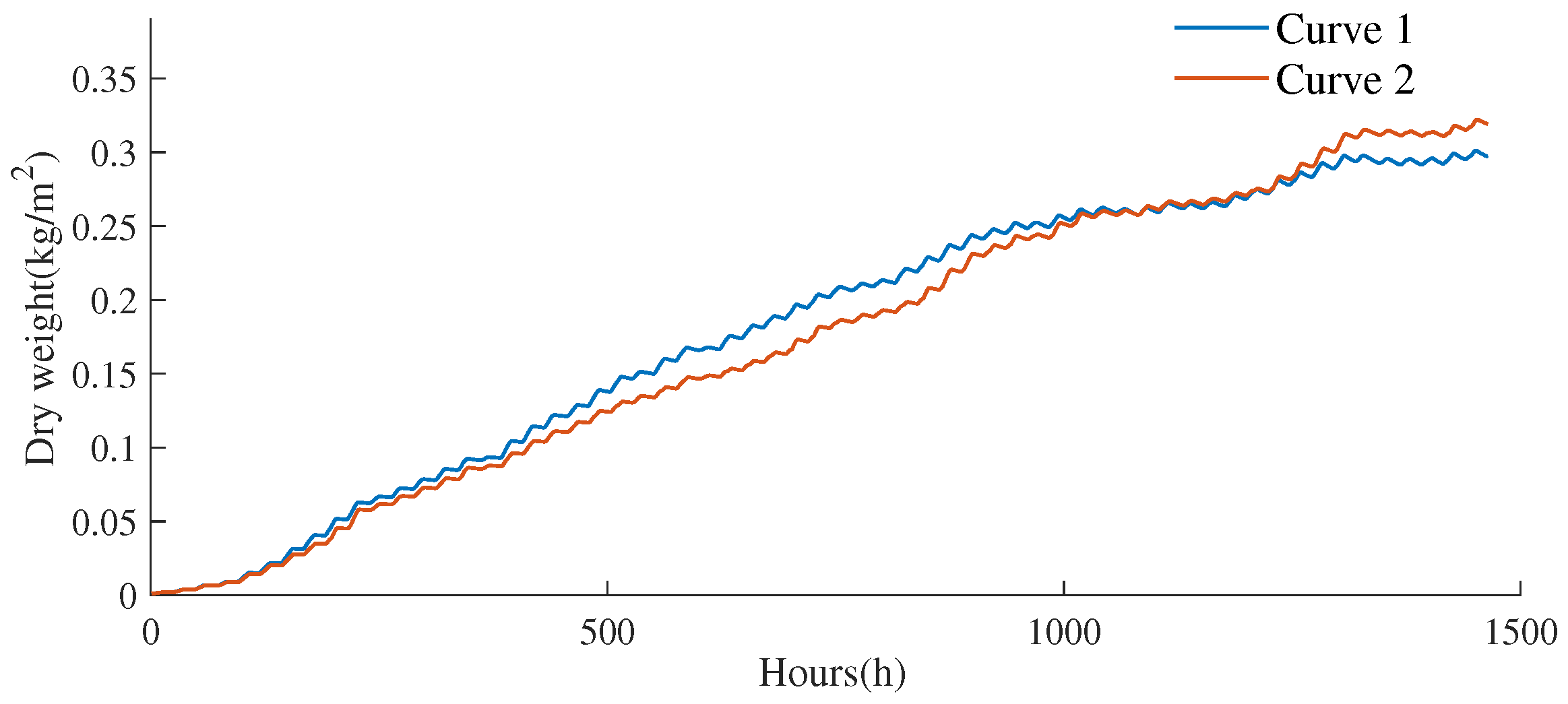
By using the switch control strategy, the reliability of the proposed mixed greenhouse model for lettuce growth trend simulation is also verified. The lettuce growth model of this paper refers to Henten’s four-state-variable model with crop dry matter as the main state variable. For this reason, the four-state-variable model [7] is constructed as a benchmark model. Using the same switch control strategy and collected external meteorological data, the dry matter growth curves under the two lettuce growth models are obtained and are shown in Figure 13. It can be seen from the figure that the crop growth curves under the two models are generally consistent.
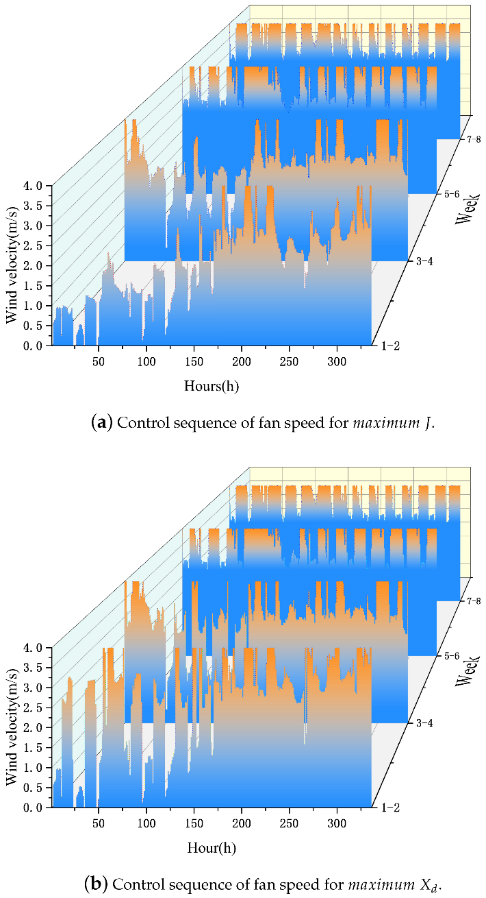
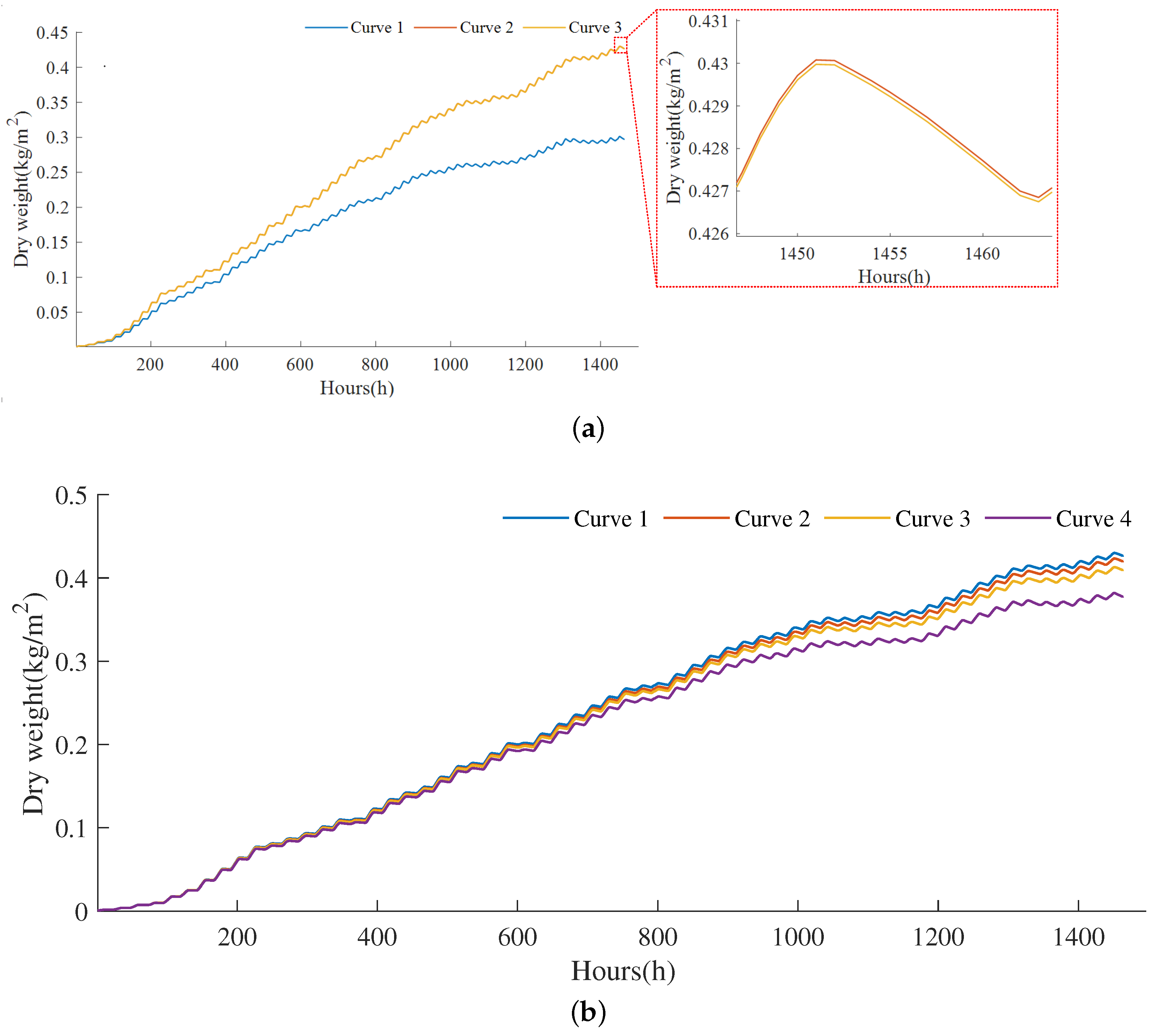
The features of the control sequences under different optimization objectives are also investigated. We change the objective function from  m a x i m u m J  to  m a x i m u m X d  and apply the same optimal control strategy again for comparison. From Figure 11, it is found that the fan-speed sequences under the two objectives are obviously different because the target of energy efficiency affects the usage of fans. The crop yield and fan energy consumption are both considered simultaneously in the objective function J. Especially in the early stage of crop growth, the fan-speed sequence under  m a x i m u m J  is much lower than that under  m a x i m u m X d . Table 4 specifies the gross profits under the two different objective functions. From the table, the proposed optimal control strategy with the objective of  m a x i m u m J  has a gross profit of RMB 12,688.17. Although the total sales of lettuce is slightly lower, the energy-saving use of fans makes the overall economic return better than that under  m a x i m u m X d  (RMB 12,678.56). Under optimal control with maximum Xd, the energy cost is RMB 92.57. Under optimal control with maximum J, the energy cost is RMB 79.80. The price of electricity is fixed, and the usage of energy is directly proportional to the energy cost: (79.80–92.57)/92.57 ≈ −13.8%; about 13.8% of the electric energy is saved. It is also noted that since only fan energy consumption is considered in  m a x i m u m J , the cost of energy consumption is disproportionately small compared with crop sales. (From Figure 14a, it is found that the crop yield curves under the two objectives are very close.) If necessary, the term of energy consumption in the objective J can be given a greater weight in the optimization process, so as to effectively strengthen the energy-saving effect. In Figure 14b, we simulate the crop yield curves under three soaring electricity prices. Table 4 also specifies their energy costs and economic benefits.
Overall, by the proposed control method, the spatial distribution of crop yield can be estimated with high resolution, and the greenhouse climate field can be optimally controlled accordingly. From the results of different control strategies, switch-control-based simple climate management has the worst economic return for crop harvest. The  m a x i m u m X d -based climate optimal control has the highest crop yields. Considering energy consumption, the proposed  m a x i m u m J -based climate control strategy is the best climate management solution in this study. By replacing CFD simulation with a real sensor matrix, this control method has the potential for engineering practice.

4.3. Assumptions and Limitations

Actually, the processes of greenhouse climate variation and crop growth are very complicated in real situations. To design the proposed optimal control strategy with low computation cost and high spacial resolution, the greenhouse crop model is simplified to some extent and has several assumptions as follows:
*
In the CFD simulations of the greenhouse climate, the temperatures of each wall and the land are considered homogeneous and constant. Considering the planting conditions of East China in summer, the concentration of carbon dioxide is simplified to a constant.
*
The timescales of greenhouse environmental variation and crop growth are unified at an hourly scale. Smaller-timescale changes are ignored.
*
Since the performance criteria are set hourly, the results of the proposed optimal control strategy are not the ideal global optimal solutions.

5. Conclusions

In this paper, an optimal control scheme for greenhouse climate management is designed. POD technology combined with CFD simulation helps achieve greenhouse climate response with high spatial resolution. A modified crop growth model is used to simulate the increase in dry weight that is mainly affected by ambient air temperature and solar radiation. With the performance criterion J of maximizing crop production and energy efficiency, the optimal control variables of greenhouse shading rate and fan speed are derived. The results indicate the proposed method’s low computation cost and high spacial resolution. Compared with the traditional switch control method, crop dry weight per square meter is increased from 0.30 kgm 2  to 0.43 kgm 2 , the total profit is increased from RMB 8888.17 to RMB 12,688.17, and the gross profit of this method is increased by 42.75%. In the comparison of two optimal control schemes with different performance criteria, the proposed strategy with objective  m a x i m u m J  saves 13.8% energy usage compared with the same control strategy with objective of  m a x i m u m X d . This method considers spatial distributions of environmental factors in the greenhouse; thus, it can help realize the optimal climate control for multi-crop planting in different zones with high accuracy and spatial resolution. By replacing CFD simulation with a real sensor matrix and also using the offline–online strategy, this control method is expected to be applied to engineering practice in the future.

Author Contributions

K.L. designed the overall framework. Y.M. developed the greenhouse CFD/POD model and performed the optimal control strategy. W.Z. prepared all data and realized part of the algorithms. All authors have read and agreed to the published version of the manuscript.

Funding

This research was funded by National Natural Science Foundation of China (grant No. 61873114), “Six Talents Peak” high-level talent program of Jiangsu Province (grant No. JZ-053), and the Youth Program of the Agricultural Equipment Faculty of Jiangsu University (grant No. NZXB20210211).

Data Availability Statement

Not applicable.

Conflicts of Interest

The authors declare no conflict of interest.

Nomenclature

PODProper orthogonal decomposition
CFDComputational fluid dynamics
CFD-POD methodRapid reconstruction of greenhouse climate environment based on CFD and
POD feature extraction
PSOParticle swarm optimization
DO modelDiscrete ordinates model
  C α β Yield factor
C c o 2 , 1 , C c o 2 , 2  , C c o 2 , 3 Temperature influence on gross canopy photosynthesis
  C p l , d Effective canopy surface
  C r a d , p h o t Light-use efficiency
  C r e s p Respiration rate expressed in terms of the amount of respired dry matter
  C Γ Carbon dioxide compensation point
  φ p h o t Gross canopy photosynthesis rate
  V r a d Solar radiation in the greenhouse
  X c Carbon dioxide concentration
  X T Temperature
  X T Crop dry weight
  P r Rated power of the fan
  N f a n Number of fans
  S f a n Rated air supply capacity of the fan
  S g h Area of the crop area
  C p r i c e , 1 Price of lettuce in the wholesale market
  C p r i c e , 2 Price of electricity
  C λ , 1 Ratio of wet weight to dry weight of lettuce
  C λ , 2 Ratio of root dry weight of lettuce to total dry weight
  Φ Converted economic benefit of crops
LEconomic cost of electrical energy consumed by the greenhouse
fan wet curtain system

References

  1. Lin, D.; Zhang, L.; Xia, X. Hierarchical model predictive control of Venlo-type greenhouse climate for improving energy efficiency and reducing operating cost. J. Clean. Prod. 2020, 264, 121513. [Google Scholar] [CrossRef]
  2. Dhiman, M.; Sethi, V.; Singh, B.; Sharma, A. CFD analysis of greenhouse heating using flue gas and hot water heat sink pipe networks. Comput. Electron. Agric. 2019, 163, 104853. [Google Scholar] [CrossRef]
  3. Van Straten, G.; Van Henten, E. Optimal greenhouse cultivation control: Survey and perspectives. IFAC Proc. Vol. 2010, 43, 18–33. [Google Scholar] [CrossRef]
  4. Jin, C.; Mao, H.; Chen, Y.; Shi, Q.; Wang, Q.; Ma, G.; Liu, Y. Engineering-oriented dynamic optimal control of a greenhouse environment using an improved genetic algorithm with engineering constraint rules. Comput. Electron. Agric. 2020, 177, 105698. [Google Scholar] [CrossRef]
  5. González, R.; Rodriguez, F.; Guzmán, J.L.; Berenguel, M. Robust constrained economic receding horizon control applied to the two time-scale dynamics problem of a greenhouse. Optim. Control. Appl. Methods 2014, 35, 435–453. [Google Scholar] [CrossRef]
  6. Van Hanten, E. Optimal control of greenhouse climate. Math. Control. Appl. Agric. Hortic. 1991, 24, 27–32. [Google Scholar] [CrossRef]
  7. Henten, E.J.V. Greenhouse Climate Management: An Optimal Control Approach; Wageningen University and Research: Wageningen, The Netherlands, 1994. [Google Scholar]
  8. Xu, D.; Du, S.; van Willigenburg, G. Adaptive two time-scale receding horizon optimal control for greenhouse lettuce cultivation. Comput. Electron. Agric. 2018, 146, 93–103. [Google Scholar] [CrossRef]
  9. Van Henten, E.; Bontsema, J. Time-scale decomposition of an optimal control problem in greenhouse climate management. Control. Eng. Pract. 2009, 17, 88–96. [Google Scholar] [CrossRef]
  10. Piscia, D.; Muñoz, P.; Panadès, C.; Montero, J. A method of coupling CFD and energy balance simulations to study humidity control in unheated greenhouses. Comput. Electron. Agric. 2015, 115, 129–141. [Google Scholar] [CrossRef]
  11. Xu, D.; Du, S.; Van Willigenburg, G. Double closed-loop optimal control of greenhouse cultivation. Control. Eng. Pract. 2019, 85, 90–99. [Google Scholar] [CrossRef]
  12. Santolini, E.; Pulvirenti, B.; Benni, S.; Barbaresi, L.; Torreggiani, D.; Tassinari, P. Numerical study of wind-driven natural ventilation in a greenhouse with screens. Comput. Electron. Agric. 2018, 149, 41–53. [Google Scholar] [CrossRef]
  13. Zhang, Y.; Yasutake, D.; Hidaka, K.; Kitano, M.; Okayasu, T. CFD analysis for evaluating and optimizing spatial distribution of CO2 concentration in a strawberry greenhouse under different CO2 enrichment methods. Comput. Electron. Agric. 2020, 179, 105811. [Google Scholar] [CrossRef]
  14. Kim, K.; Yoon, J.Y.; Kwon, H.J.; Han, J.H.; Son, J.E.; Nam, S.W.; Giacomelli, G.A.; Lee, I.B. 3-D CFD analysis of relative humidity distribution in greenhouse with a fog cooling system and refrigerative dehumidifiers. Biosyst. Eng. 2008, 100, 245–255. [Google Scholar] [CrossRef]
  15. Katzin, D.; van Henten, E.J.; van Mourik, S. Process-based greenhouse climate models: Genealogy, current status, and future directions. Agric. Syst. 2022, 198, 103388. [Google Scholar] [CrossRef]
  16. Sempey, A.; Inard, C.; Ghiaus, C.; Allery, C. A state space model for real-time control of the temperature in indoor space-principle, calibration and results. Int. J. Vent. 2008, 6, 327–336. [Google Scholar]
  17. Li, K.; Xue, W.; Xu, C.; Su, H. Optimization of ventilation system operation in office environment using POD model reduction and genetic algorithm. Energy Build. 2013, 67, 34–43. [Google Scholar] [CrossRef]
  18. Tan, B.T. Proper Orthogonal Decomposition Extensions and Their Applications in Steady Aerodynamics. Master’s Thesis, Singapore-MIT Alliance, Singapore, 2003. [Google Scholar]
  19. Tallet, A.; Allery, C.; Allard, F. POD approach to determine in real-time the temperature distribution in a cavity. Build. Environ. 2015, 93, 34–49. [Google Scholar] [CrossRef]
  20. Lieu, T.; Farhat, C.; Lesoinne, M. Reduced-order fluid/structure modeling of a complete aircraft configuration. Comput. Methods Appl. Mech. Eng. 2006, 195, 5730–5742. [Google Scholar] [CrossRef]
  21. Wang, X.; Zhao, J.; Wang, F.; Song, B.; Zhang, Q. Air supply parameter optimization of a custom nonuniform temperature field based on the POD method. Build. Environ. 2021, 206, 108328. [Google Scholar] [CrossRef]
  22. Munar, E.; Bojaca, C.; Baeza, E. Transient CFD analysis of the natural ventilation of three types of greenhouses used for agricultural production in a tropical mountain climate. Biosyst. Eng. 2019, 188, 288–304. [Google Scholar]
  23. Li, K.; Sha, Z.; Xue, W.; Chen, X.; Mao, H.; Tan, G. A fast modeling and optimization scheme for greenhouse environmental system using proper orthogonal decomposition and multi-objective genetic algorithm. Comput. Electron. Agric. 2020, 168, 105096. [Google Scholar] [CrossRef]
  24. Jolliffe, I.T.; Cadima, J. Principal component analysis: A review and recent developments. Philos. Trans. R. Soc. A Math. Phys. Eng. Sci. 2016, 374, 20150202. [Google Scholar] [CrossRef] [PubMed]
  25. Li, K.; Xue, W.; Mao, H.; Chen, X.; Jiang, H.; Tan, G. Optimizing the 3D distributed climate inside greenhouses using multi-objective optimization algorithms and computer fluid dynamics. Energies 2019, 12, 2873. [Google Scholar] [CrossRef]
  26. Xu, D.; Ahmed, H.A.; Tong, Y.; Yang, Q.; Willigenburg, L.V. Optimal control as a tool to investigate the profitability of a Chinese plant factory—Lettuce production system. Biosyst. Eng. 2021, 208, 319–332. [Google Scholar] [CrossRef]
  27. Xu, K. Fan Manual; China Machine Press: Beijing, China, 2011. [Google Scholar]
  28. Ratnaweera, A.; Halgamuge, S.K.; Watson, H.C. Self-organizing hierarchical particle swarm optimizer with time-varying acceleration coefficients. IEEE Trans. Evol. Comput. 2004, 8, 240–255. [Google Scholar] [CrossRef]
  29. Engelbrecht, A.P. Particle swarm optimization with crossover: A review and empirical analysis. Artif. Intell. Rev. Int. Sci. Eng. J. 2016, 45, 131–165. [Google Scholar] [CrossRef]
  30. Song, C.Y.; Jiang, M.C.; Shi, H.J.; Jiang, Y.Q.; Jiang, J.Q.; Bao, D.X. Particle Swarm Optimization Algorithm and Its Application. J. Inn. Mong. Univ. Natl. (Nat. Sci.) 2006, 29, 2531–2561. [Google Scholar]
  31. Tang, J.; Liu, G.; Pan, Q. A Review on Representative Swarm Intelligence Algorithms for Solving Optimization Problems:Applications and Trends. IEEE/CAA J. Autom. Sin. 2021, 8, 17. [Google Scholar]
  32. Kittas, C.; Bartzanas, T. Greenhouse microclimate and dehumidification effectiveness under different ventilator configurations. Build. Environ. 2007, 42, 3774–3784. [Google Scholar] [CrossRef]
  33. Fidaros, D.K.; Baxevanou, C.A.; Bartzanas, T. Numerical simulation of thermal behavior of a ventilated arc greenhouse during a solar day. Renew. Energy 2010, 35, 960–1481. [Google Scholar] [CrossRef]
  34. Wen, Z.; Shi, L.; Ren, Y. FLUENT Fluid Mechanics Calculation Application Textbook; Tsinghua University Press: Beijing, China, 2009. [Google Scholar]
  35. Al-Said, F.; Hadley, P.; Pearson, S.; Khan, M.M.; Iqbal, Q. Effect of high temperature and exposure duration on stem elongation of iceberg lettuce. Pak. J. Agric. Sci. 2018, 55. [Google Scholar]
  36. Zhou, J.; Li, P.; Wang, J.; Fu, W. Growth, photosynthesis, and nutrient uptake at different light intensities and temperatures in lettuce. HortScience 2019, 54, 1925–1933. [Google Scholar] [CrossRef]
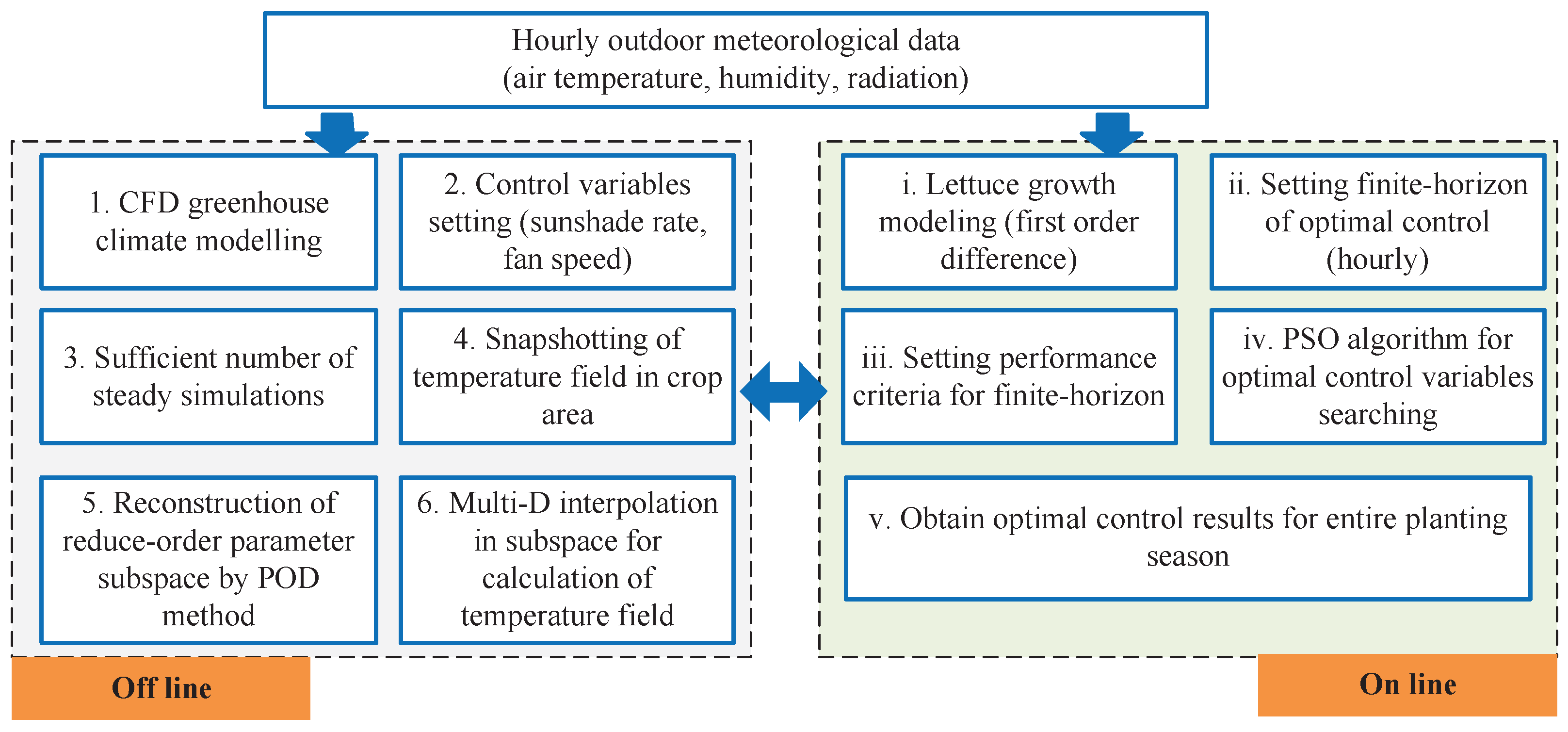
Figure 1. The overall optimal control framework.
Energies 16 03925 g001
Figure 2. The test greenhouse’s location and structure.
Energies 16 03925 g002
Figure 3. CFD model of greenhouse with mesh grids.
Energies 16 03925 g003
Figure 4. Residual diagram of CFD greenhouse modeling.
Energies 16 03925 g004
Figure 5. Temperature contours at X–Z section (0.3 m high) of greenhouse for three fan speeds: 0 m/s, 2 m/s and 4 m/s.
Energies 16 03925 g005
Figure 6. Meteorological data of the greenhouse: outdoor relative humidity (upper), air temperature (middle) and solar radiation (bottom) from 0:00 of 1 May to 23:00 of 30 June 2021.
Energies 16 03925 g006
Figure 7. The 135 evenly selected sample-point locations in the four environmental parameters’ space.
Energies 16 03925 g007
Figure 8. The first two principal mode coefficient distributions corresponding to four variables: (a) the 1st mode coefficient’s distribution; (b) the 2nd mode coefficient’s distribution.
Energies 16 03925 g008
Figure 9. Schematic of particle swarm searching process:  D a t a 1  represent the original distribution of the particle swarm, and  D a t a 2  represent the distribution after five iterations.
Energies 16 03925 g009
Figure 10. Spatial distributions of crop yields under different control strategies: (a) proposed optimal control and (b) switch control.
Energies 16 03925 g010
Figure 11. Optimal control sequences of fan speed for different objective functions: (a m a x i m u m J  and (b m a x i m u m X d .
Energies 16 03925 g011
Figure 12. Optimal control sequence of sunshade rate for  m a x i m u m J .
Energies 16 03925 g012
Figure 13. Simulated curves of crop dry weight per unit using the same switch control strategy and external meteorological data: Curve 1 represents the result of the proposed model, and Curve 2 represents the result of the four-state-variable model from [7].
Energies 16 03925 g013
Figure 14. Simulated curves of crop dry weight per unit using different control strategies and energy costs: (a) simulated curves representing different control strategies and (b) simulated curves representing different electricity prices. (a) Simulated curves of crop dry weight per unit using three control strategies: Curve 1 represents the result of switch control, Curve 2 represents the result of optimal control with  m a x i m u m X d , and Curve 3 represents the result of optimal control with  m a x i m u m J . (b) Simulated curves of unit crop dry weight per unit using four electricity prices: Curve 1 represents current electricity price, Curve 2 represents  5 ×  current price, Curve 3 represents  10 ×  current price, and Curve 4 represents  50 ×  current price.
Energies 16 03925 g014
Table 1. Initial/correlation coefficients of greenhouse lettuce growth model.
ParameterValue
  C α β 0.544
  C c o 2 , 1   5.11 × 10 6 m s 1   C 2
  C c o 2 , 2   2.30 × 10 4 m s 1   C 1
  C c o 2 , 3   6.29 × 10 4 m s 1
  C p l , d   53 m 2 kg 1
  C r a d , p h o t   3.55 × 10 9 kg J 1
  C r e s p   2.65 × 10 7 s 1
  C Γ   5.2 × 10 5 kg m 3
  X c   6.41 × 10 4 kg m 3
  P r   0.55 kWh
  N f a n 3
  S f a n   3 × 10 5 m 3 h 1
  S g h   6.08 × 10 2 m 2
  C p r i c e , 1   1.5 RMB kg 1
  C p r i c e , 2   0.5283 RMB kWh 1
  C λ , 1   22.5
  C λ , 2   1.69 × 10 1
Table 2. Physical property parameters of greenhouse materials.
MaterialDensitySpecific Heat Cap.Thermal Cond.Absorption Coef.Refractive
( kg m 3 )( J kg 1 K 1 )( W m 1 K 1 )( m 1 )Index
Porous material70023100.170.262.77
Land190022001.150.51.5
Float glass25007000.710.11.7
Table 3. Main parameter settings for optimal control.
ParameterValue or Range
Control variable 1fan speed (0–4  ms 1 )
Control variable 2sunshade rate
External meteorological dataair temperature, relative humidity and solar radiation
(East China from 1 May to 30 June 2021)
Control time horizon8 weeks
Time stephourly
Control targetdry weight increase and energy efficiency
Optimization algorithmPSO algorithm
Particle number100
Iteration number5
Number of POD modes6
Table 4. Effects of different control strategies on crop growth, energy consumption and economic benefits.
StrategyDry Weight,Wet Weight,Selling Price,Energy Cost,Gross Profit,
kg/m 2 kg/m 2 RMBRMBRMB
Switch control0.306.238898.5510.388888.17
Optimal control
(maximum  X d )≈ 0.43≈ 8.9412,771.1392.5712,678.56
Optimal control
(maximum J)   0.43   8.94 12,767.9779.8012,688.17
Optimal control
(maximum J 5 ×
electricity price)   0.42   8.80 12,568.0479.8012,405.41
Optimal control
(maximum J 10 ×
electricity price)   0.41   8.57 12,251.78188.4812,063.30
Optimal control
(maximum J 50 ×
electricity price)   0.38   7.91 11,297.56180.2511,117.32
Disclaimer/Publisher’s Note: The statements, opinions and data contained in all publications are solely those of the individual author(s) and contributor(s) and not of MDPI and/or the editor(s). MDPI and/or the editor(s) disclaim responsibility for any injury to people or property resulting from any ideas, methods, instructions or products referred to in the content.