Abstract
Tidal energy resource characterisation using acoustic velocimetry sensors mounted on the seabed informs developers of the location and performance of a tidal energy converter (TEC). This work studies the consequences of miscalculating the established flow direction, i.e., the direction of assumed maximum energy yield. Considering data only above the proposed TEC cut-in velocities showed a difference in the estimated flow direction of up to 4°. Using a power weighted rotor average (PWRA) method to obtain the established flow direction resulted in a difference of less than 1° compared with the hub-height estimate. This study then analysed the impact of turbine alignment on annual energy production (AEP) estimates for a non-yawing tidal turbine. Three variants of horizontal axis tidal turbines, which operate in different locations of the water column, were examined; one using measured data, and the other two via modelled through power curves. During perfect alignment to the established flow direction, natural variations in flow meant that the estimate of AEP differed by up to 1.1% from the theoretical maximum of a fully yawed turbine. In the case of misalignment from the established flow direction, the difference in AEP increased. For a 15° misalignment, the AEP differed by up to 13%. These results quantify important uncertainties in tidal energy site design and performance assessment.
1. Introduction
Tidal-stream energy, the extraction of kinetic energy from tidal currents to generate electricity, is becoming an increasingly attractive form of renewable energy due to the high predictability of the tides [1,2,3]. This resource has the potential to provide energy security and support a renewable grid network shift to decarbonised energy generation. Initial feasibility studies and characterisation of high energy sites often focus on peak velocity (>2.5 m·s) and a restricted range of water depths (25–50 m) [1,4,5]. However, peak values do not accurately indicate the potential power production due to fine-scale temporal and spatial variability in the flow. Therefore, gathering additional information from site resource characterisations, while using Acoustic Doppler Current Profilers (ADCPs), is vital for understanding the potential uncertainties. In addition to quantifying the available resource, evaluating the tidal energy converters’ (TECs) performance in natural conditions is challenging. Still, it remains an essential aspect of accelerating the tidal industry to the commercialisation phase [6].
Most TECs frequently developed do not have the ability to actively respond to changes in the current direction [7]. Thus, are of a non-yawing (no rotation in the nacelle) horizontal axis design, [8,9,10,11,12,13], some designs yaw ≈ four times a day to face perpendicular to the established flow direction, e.g., the 1 MW DEEP-Gen IV from Alstom [14,15]. However, the tidal current magnitude and direction are typically asymmetric in highly energetic tidal test sites [3,4,16,17], particularly in nearshore environments where the topography and bathymetry vary significantly [4,5]. Despite that, resource assessments commonly assume that the proposed TEC will always be aligned with the instantaneous tidal flow [4,5].
The International Electrotechnical Commission (IEC) Technical Specification (TS) on Power Performance Assessment (PPA) [18] provides guidance for collecting potential uncertainties associated with the measurement of current and power produced by TECs [18]. However, due to the limited number of grid-connected commercial-scale TECs deployed (in the UK [6,10,19], France [8,12] and the US [12,20]), the standard IEC62600-200 has been applied only to a limited number of turbines and, as a consequence, industry has limited feedback on the use of the IEC62600-200. Typically, a PPA is undertaken as a key step towards achieving type certification of the TEC [6], providing a basis to guarantee the power performance of the device to interested parties, e.g., customers, investors and insurers [21].
As part of the Reliable Data Acquisition Platform for Tidal (ReDAPT) project [22], multiple ADCP deployments took place at the European Marine Energy Centre (EMEC) full-scale tidal test site at Eday, the Fall of Warness (FoW), between 2011 and 2015. The aims were to assess the flow characteristics and evaluate in situ measurements for the power performance of the DEEP-Gen IV 1 MW tidal turbine. The location of the tidal test site is presented in Figure 1a,b. Part of this work identified a twist in the flow along the water column, where the current direction changed significantly through the water column by as much as 10° from the calculated mean [14]. At present, the flow direction measured by the ADCP depth bin relative to the proposed TEC should be reported as per IEC62600-200 [18]. Figure 1c presents the typical flow conditions at the tidal test site situated at the FoW, taken from one of the ReDAPT measurement campaigns [19]. Flow velocity and direction vary with depth—from bathymetry, seabed friction and interactions from the wind and waves. If this variation could be captured along the rotor plane of a TEC, a more accurate representation of the established flow could be estimated. This is performed for the flow velocity, using the power-weighted rotor average (PWRA) method [18], as shown in Figure 2.
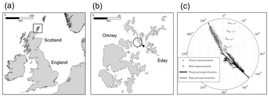
Figure 1.
Location of the study site. (a) Orkney location relative to the UK [23]; (b) The Orkney Islands with Eday and the falls of Warness full-scale tidal energy test site highlighted [23]; (c) Tidal ellipse of data used from one instrument deployed at the FoW, flood (black marker) and ebb (grey marker) flow directions are shown.
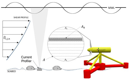
Figure 2.
The vertical variation of tidal current across the projected capture area—introducing the importance for the power PWRA technique.
Studies have analysed the impact of flow misalignment on tidal turbines. For example, Polagye and Thomson [24] used observations from an ADCP on a single point mooring to assess individual locations within Admiralty Inlet (Puget Sound, Washington, WA, USA) and estimated that the mean potential power generated by the non-yawing device may be, at most, 5% lower than for a passive yaw device at the same site. It was observed that the penalty for using non-yawing devices increases as directional variation in the flow increases [24], which agrees with work from Galloway and Frost et al. [4,25], where they suggest that power reductions may only become apparent above a certain threshold of misalignment (>7.5° with an approximately 7% reduction of peak power at ±10° directional misalignment, and a 20% reduction at 22.5°. Frost et al. [4] found that asymmetrical regimes (difference in peak velocity between the flood and ebb tidal cycle) lead to unequal power generation during the two tidal cycles. Since turbine power output is proportional to the cube of the flow velocity, even a slight difference in the velocity magnitude between tides can lead to a significant alteration in the power generated [26]. In addition, Piano et al. [5] found that optimising turbine orientation to specific flow dynamics could reduce the potential losses by up to 2% where strong asymmetry occurs and as low as 0.25% for ideal symmetrical conditions when considering a non-yawing TEC. However, tidal characteristics are dissimilar across sites and have the potential for increased losses in annual energy yield, exceeding 2% where the optimal orientation of non-yawing devices is ignored [5].
From the initial TEC concepts to the first pre-commercial tidal turbine prototypes, a key requirement has been reliability and survivability [27]. The impact of turbulence on the performance and loading acting on a tidal turbine has received little consideration to date. Turbulence describes the chaotic motions within a fluid flow and can result in fluctuations in force, which is detrimental to the fatigue life of the turbine [27,28]. The presence of the turbine can increase the turbulence and vortices generated [27,29]. Although this is recognised, and these effects can change the flow characteristics at the turbine location, this is not the focus of this study due to instrument placement and resolution.
The flow direction matures over a tidal cycle. This effect on power performance has not yet been quantified. Not knowing the impact on power will lead to an inaccurate assessment of performance. This study aims to use in situ measurements obtained from two ADCPs deployed at the FoW (Orkney, Scotland, UK) to quantify the impact off-axis currents have on power production. In addition, the impact on performance and energy yield from a rotor misalignment for three horizontal axis tidal turbines situated at different depths is assessed. This work will inform developers on turbine installation design criteria by highlighting how the temporal variation in the flow direction can result in a misalignment between the current flow and turbine extraction plane. The methods used in this study can be applied to in situ data gathered at different tidal test sites that exhibit complex magnitude and directional asymmetries to maximise potential energy yields and help interpret performance results more accurately. A method for estimating the established flow direction to inform tidal developers on turbine orientation is reported. The variation in flow direction at different depths is necessary to predict the loading effects caused due to being positioned off-axis to the established flow direction. We investigate the relative impact of current flow maturity on the power performance of non-yawing TEC concepts. We then investigate the misalignment of the turbine axis with the established flow to assess the impact on the measured power curve, and AEP estimates. As numerous tidal turbines exist and occupy different regions of the water column, three variants of a horizontal axis tidal turbine were chosen for a case study to investigate the impact of flow direction variation on machines with different operational characteristics. We suggest the optimum period for utilising a yaw mechanism by interpreting the results.
This paper is structured as follows: Section 2 introduces the theory behind the power-weighted rotor average method. In addition, the characteristics of flow direction asymmetry and maturity are presented; Section 3 describes the FoW deployment site conditions, as well as the instrumentation relevant to this work; while Section 4 reports the results on the estimates of established flow direction (Section 4.1) and the consequences of misalignment. The analysis is then presented, which considers the impact on the measured power curve (Section 4.2) and annual energy estimates with respect to off-axis currents approaching the TEC (Section 4.2.3); Section 5 presents the discussion around the hypothesis and results generated. The main conclusions from this analysis are summarised in Section 6.
As this paper discusses the impact of flow direction estimates, some abbreviations will be used throughout this paper. Where all the measured flow velocities are assumed to flow through the TEC extraction plane for maximum energy capture was referred to as ; the established flow direction estimate was and the methods used to obtain the estimate were, (hub-height), (rotor average) and (power-weighted rotor average); the misalignment from the established flow direction is represented as .
2. Theory
2.1. Estimate of Established Flow Direction—PWRA
Efforts to advise developers on how to record and report the flow direction at tidal stream sites have been made by IEC/TS 62600-200—“Electricity producing tidal energy converter—power performance assessment” [18]. This TS describes a method for ascertaining the flow characteristics of a site, which underpins the prediction of the potential resource and defines the local flow conditions and associated design considerations. Currently, the TS requires the established flow direction to be reported for the profiler bin relative to the hub-height () of the proposed TEC, along with instantaneous measurements for both the flood and ebb (see Figure 1a) [4,18].
Tidal turbines with no yaw capabilities are deployed facing the established flow direction with the most significant velocities. If the TEC is equipped with bi-directional blades, it can capture energy from current flow travelling from two opposing directions. However, highly energetic tidal sites typically have asymmetrical tides in both velocity magnitude and direction [4]. Therefore, a robust estimate of the established flow direction will inform the TEC orientation and increase power performance and quality while reducing the total loads experienced on the rotor due to off-axis currents. The established flow direction is an average of the measurements captured at the hub-height of the deployed TEC. The reference velocity is calculated from the relative profiler bins that profile across the rotor extraction plane as shown in Equation (1):
where i is the index number defining the velocity bin; j is the index number of the time instant at which the measurement is performed; k is the index number of the current profiler bin across the projected capture area (reflected in Figure 2 as ); S is the total number of current profiler bins across the projected capture area; is the instantaneous power weighted tidal current velocity across the projected capture area in m·s; is the magnitude of the instantaneous tidal current velocity, for time j, at current profiler bin k, in velocity bin i, for data point n in m·s and A is the projected capture area of the proposed TEC m.
2.2. Flow Direction Asymmetry between Flood and Ebb Tides
A tidal ellipse plot presents the velocity magnitudes (as a radius) and directions (as a compass heading) in polar coordinates. The velocity data points are typically 5, 10 or 15 min temporally averaged and spatially averaged (cube weighted) over the predicted swept area of a turbine. These plots help determine the flow magnitude and direction variation at the site of interest and identify the established flow direction to inform turbine developers. If the flow direction for the ebb and flood tidal cycles are separated by ≈180°, the site is described as symmetrical or rectilinear. Otherwise, the flow is described as asymmetrical. The amount of asymmetry between the ebb and flood tide can be summarised by computing the difference between the mean angle of both directions over a complete lunar cycle (Equation (3)). Symmetrical sites are desirable as turbines can be mounted in a fixed position, pitching the blades to capture the tides from both directions with little or no loss of power. Sites with an offset between the ebb and flood tide may benefit from a turbine that could yaw to capture both tides efficiently [4,30].
where is the angle in degrees (°).
2.3. Flow Direction Variation a Tidal Cycle
In addition to asymmetrical tides, the flow direction changes during the different phases of the tide. As the tide evolves to the established flow direction, this will be referred to as the ramping up (RU) of the tide, and as the tide begins to slow from peak flow (PF) before changing tide, this phase will be referred to as waning down (WD), as seen in Figure 3. For non-yawing TEC concepts, the ability to capture the largest amount of energy will only take place once the TEC is positioned perpendicular to the flow. This variation in direction results in a reduced velocity passing through the TEC rotor capture area. Hence, this must be considered when evaluating and producing a measured power curve.
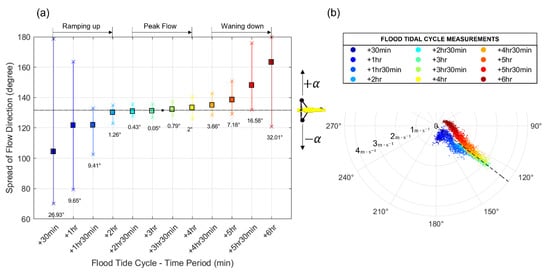
Figure 3.
Flow direction variation over a flood tide at the FoW, where (a) the flow direction mean (square markers) of 30 min periods throughout the flood cycle, the TEC yaw heading (solid black line) and the min and max (crosses) variation in direction. (b) The tidal ellipse for the flood measurements at a chosen hub-height (25 m), the black dashed line represents the TEC yaw heading.
Figure 3 depicts how flow varies with time during a flood cycle at the instrument location (direction measurements are subject to variation based on instrument location) in the FoW.
The measured flow evolves and a non-yawing TEC positioned towards the established flow direction will be susceptible to off-axis currents throughout each tidal cycle. Equation (4) describes the inflow velocity () at the instrument location, and the velocity at the TEC location () when the turbine’s rotor heading is perpendicular to the free stream flow at all times (), thus capturing the maximum amount of energy available. In misalignment circumstances, the inflow velocity becomes a component of the velocity, and the parameter quantifies the difference between and . The impact of misalignment can be described using a simple trigonometric cosine relationship [4], as shown in Equation (5):
Alternatively, the turbine’s swept area can be considered when misalignment is introduced and it changes from a circle to an ellipse. The vertical radius of the ellipse will remain the same, and the horizontal radius will decrease as the yaw angle increases from the established flow direction. The resulting equation for a turbine’s projected area in aligned and misaligned flow is described by Equations (6) and (7), respectively, as shown below:
where r is the radius of the turbine and is the misalignment in degrees between the and .
It is expected that either one of these two corrections, when applied to the theoretical maximum power equation, may estimate the performance drop due to misalignment. Tidal stream devices designed to react to tidal sites with asymmetrical tides may lack the sufficient ability to extract energy efficiently from off-axis currents. The maximum power can be calculated using Equation (8):
where P is the power produced in MW, is the density of water in kg·m, is the power coefficient, U is the instantaneous flow velocity in m·s and A is the cross-sectional area of the TEC rotor in m.
3. Methodology
3.1. Deployment Site Conditions
A measurement campaign was devised to assess the DEEP-Gen IV 1 MW tidal turbine performance using two ADCPs over June and July 2013 at the FoW (Figure 1). The full-scale tidal test site situated on the coast of Eday contains highly energetic tidal currents due to a narrowing of the channel between Eday and Muckle Green Holm, a small outcrop southwest of the island. Figure 4 presents the channel bathymetry and instrument locations. The tidal current flows southeast and northwest throughout the flood and ebb tide, respectively. The strength in the ebb tide at the FoW is larger and less spatially varied, reaching a PF of 4 m·s with a flow direction spread of ≈35° from the RU to WD phase. The flood tide reaches a PF of ≈3.2 m·s with a much larger flow direction spread of ≈75°. The flood tide is more turbulent due to the flow being disturbed by several features, including the site bathymetry and nearby headlands [31]. For the following performance assessment, results obtained in both tidal cycles are considered as the flow direction spread differs between tidal cycles.
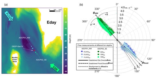
Figure 4.
(a) Channel bathymetry and ADCP locations relative to the DEEP-Gen IV at the FoW tidal test site. (b) Tidal ellipse for three bin depths, where , and represent 15, 25 and 33 m above the seabed. The generic established flow direction for both flood and ebb is presented. TEC yaw heading rotations used throughout the analysis are illustrated, where both clockwise and anticlockwise rotations are considered (). NOTE measurements shown indicate flow travelling towards that direction.
The variation in flow direction at different heights above the seabed over each tidal cycle is dissimilar. Therefore, three TEC concepts that occupy different regions of the water column were chosen to assess the impact of power performance relative to the amount of time spent off-axis to the established flow. Figure 4b depicts the measurements along the water column at three depths. The flow direction is not symmetrical from the RU phase to the PF phase and further during the WD phase (clockwise and anti-clockwise from the established flow direction). Therefore, the analysis considers both positive ( and negative ( rotations of the TEC yaw to the established flow estimate () seen in Figure 3 and Figure 4b.
3.2. Instrumentation and Turbine Description
In situ measurements were made using Tenedyne RDI workhorse 600 kHz, with four-beam ADCPs, fixed into gimbal support on a seabed frame. The locations of the ADCPs were known to the nearest meter based on their Universal Transverse Mercator (UTM) coordinates, see Table 1. Using a bathymetric map with each ADCP pressure data, their depths relative to the TEC were estimated to the nearest meter (as the ADCPs were set up with a resolution of 1 m).

Table 1.
ADCP deployment specifications, showing the campaign ID, date deployed (dd-mm-yyyy) and deployment duration. The position is UTM Zone 30 N.
Three TEC concepts were used to model the impact of misalignment between the flow direction and TEC rotor on the measured power curve. These models are based on work carried out in the RealTide advanced monitoring, simulation and control of tidal devices project [32], where TEC represents the DEEP-Gen IV which is used for this study (Table 2). They have different operational characteristics and are deployed in distinct regions in the water column; see Table 3 for turbine dimensions and operational specifications.
Table 2.
Generic tidal turbine concepts and features [32].
Table 3.
TEC operational characteristics and location in the water column.
3.3. Data Processing
All post-processing was applied to the data conformed to IEC/TS 62600-200 [18]. Each instrument was processed with the same suite of methods and recommended measures were based on internationally recognised QARTOD guidelines and the ADCP manufacturer’s best practices [33,34,35]. Measurements that lay outside the thresholds were flagged and removed from the analysis. The IEC suggests using an averaging period between 2 and 10 min; the latter has been used for this analysis.
The measurement campaign used in this study featured periods with no generated power or inconsistent generation from the DEEP-Gen IV, reducing the amount of comparable data. For that reason, power was calculated using the published power curve provided by Alstom (for the mid-depth TEC concept). Each velocity measurement was allocated an active power value from the pre-defined power curve for the DEEP-Gen IV 1 MW TEC [19]. In addition, two separate power curves were produced to simulate power production for the 0.25 MW and 2 MW TEC concepts. To illustrate the method, see Equation (9):
where is the predefined rated power, U is the in situ velocity measurement in m·s, is the cut-in velocity for the proposed TEC and is the rated flow velocity for peak power production. Velocity measurements that fall beneath the cut-in are rejected, and above the rated are equal to the rated power defined.
The PWRA technique was used to calculate the two bottom-fixed TEC concepts (insufficient data in the upper depth bins meant this technique was not usable) using Equation (1). This was paired with the corresponding power produced. The following steps were then performed using the bin methodology:
- Calculate the mean value of the velocity, and the respective data sources (TEC power), aswhere is the number of samples in the defined averaging period which produces data point n.
- Sort values into the corresponding flow velocity bin—increments of 0.1 m·s
The energy production was estimated from each instrument’s available time series power data. This was derived via the trapezoidal method, which computes the approximate power integral. The energy was then multiplied by the deployment campaign’s ratio to the year’s length, as seen in the following Equation (12):
where is the expected annual energy production, in MWh, R is the ratio of the number of days a year over the duration of the deployment, is the mean calculated TEC power, is the index number defining the time start and is the index number of the end time interval.
4. Results
4.1. Estimates of the Established Flow Direction
Table 4 shows the effect of inclusion of data measured beneath the cut-in speed when calculating the established flow direction. Differences of up to 4° can be seen without removing data under the proposed TEC cut-in speed. The estimate of the established flow calculated using flow direction measurements aligned to the rotor plane (rotor average), alongside the PWRA method, exhibited a less than 1.2° difference, when compared with the commonly used hub-height estimate (Table 4). Shown also in Table 4, the estimate of the established flow direction varied across the three depths by up to 4°. This highlights an area where uncertainties may occur in using an ADCP for flow characterisation, causing potential issues, for example, if they are used to instruct turbine heading.
Table 4.
Effect of pre-processing on the estimate of established flow direction.
Flow Variation along the Water Column
The 10 min averaged measurements were split by the acceleration and deceleration of the tide, and into velocity bin increments of 1 m·s. Figure 5a,b shows a variation with depth in the flow direction along the measured water column of ≈8° and 13° for the ebb and flood tide at peak flow (3–4 m·s), respectively. Shown also in Figure 5a,b, the estimate of (solid red line) and (red cross), differed by ≈0.9% at locations TEC (presented in Figure 5) and TEC.
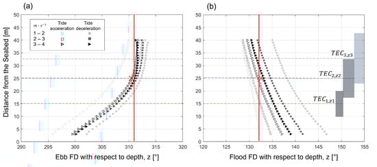
Figure 5.
Flow direction variation along the measured water column (z) during the acceleration and deceleration phase of the tide for (a) the ebb tide measurements and (b) the flood tide measurements. The established flow direction estimate using (solid red line) and (red cross) methods are shown for TEC. The position of all three TECs in the water column are shown in (b).
Figure 5b depicts the variation in flow direction in the lower region (<15 m) as ≈11–13°, compared to ≈5–7°, in the upper region (>35 m from the seabed) on the flood tide. The ebb tide ranged from ≈6° down to 4° between the lower and upper region, as shown in Figure 5a. This highlighted that the two tidal cycles have different flow direction characteristics and that the acceleration and deceleration phases of the tide differ significantly between the flood and ebb tidal cycles.
4.2. Consequence of Misalignment on Performance Metrics
4.2.1. Axial Rotation Impact
The probability density distribution of flow direction, as shown in Figure 6, depicts how the flow direction evolves over a tidal cycle. The density curves are right-skewed, with the mean estimation greater than the median. The flow direction spends the majority of the time clockwise from the established flow direction (towards the waning down phase) of the tide for both tidal cycles. This highlighted that a TEC positioned off-axis from the established flow by either a positive (clockwise) or negative (anti-clockwise) shift would not perform identically.
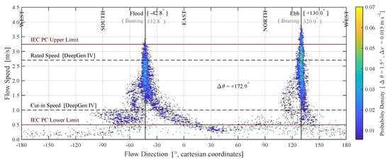
Figure 6.
Probability density distribution for varying flow speeds and flow directions (in cartesian coordinates) for flood and ebb tides. The data have been generated from hub-height measurements sampled by an ADCP deployed ≈40 m south-west of the DEEP-Gen IV TEC (in a region of flow undisturbed by the presence of the turbine) [36,37]. The ADCP dataset is available at [38].
4.2.2. Impact of Misalignment on the Power Performance
Figure 7a shows the generated power output for each 10 min measurement against the flood tide velocity component approaching the DEEP-Gen IV. The theoretical maximum power (red line) generated using the velocity magnitude was compared with the velocity component , where is the streamwise misalignment between the TEC heading and established flow estimate () of 5°, 10° and 15°. As shown in Figure 7a, the DEEP-Gen IV curves differed by up to ≈1.5%, 4.9% and 10% at 2.5 m·s for a misalignment of 5°, 10° and 15°. Figure 7b–d depicts the power loss for each TEC case when misaligned from the established flow, where the highest value of power lost per velocity bin was measured from TEC. At lower flow velocities, more visible differences exist between the curves presented in Figure 7b–d. This is due to the variation between the 10 min samples of flow direction and the averaged established flow direction varying significantly more during low flow speeds, thus causing a greater misalignment.
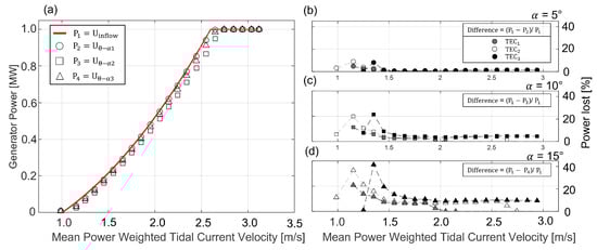
Figure 7.
Comparison of theoretical maximum power generated using (red line) and the realistic power generated using velocity component , where the TEC is misaligned to the established flood direction. The DEEP-Gen IV power curve is presented (a) by the unfilled symbols, where the circle, square and triangle represent a misalignment from the established flow of 5° (b), 10° (c) and 15° (d), respectively. Filled symbols represent the percentage lost in power when flow data used features misalignment for TEC (filled grey) and TEC (filled black).
The power lost from ebb measurements was lower than the flood measurements (Figure 7). This is due to narrower flow direction spread (≈35°) at this location and the greater occurrence of the flow velocity exceeding (3.9 m·s), the TECs-rated velocities. However, due to this narrow flow direction spread, the impact on the power curve was more severe when the flow data used were a velocity component due to misalignment from the established flow direction.
4.2.3. Consequence to AEP
Figure 8 is a graphical representation of the difference in AEP estimates when changing the TEC heading away from the established flow direction. It can be seen that the introduction of misalignment reduces the total amount of energy captured and by different amounts when misaligned clockwise or anti-clockwise to the established flow direction. The greatest loss in AEP, when compared against the theoretical maximum, was found when the TEC was positioned clockwise from the established flow direction on the ebb tide. The results differed by up to 7.8%, 10.1% and 13.3% for TEC, TEC and TEC, respectively. A summary of the AEP losses found is provided in Table 5. The natural variation in flow direction measured on the ebb tide is closer to the established flow direction, resulting in a lower AEP loss of ≈0.7%, 0.8% and 1.1% when TEC, TEC and TEC are accurately aligned with the established flow direction . However, when the TEC is not aligned to , the AEP losses are significantly greater when compared with a misalignment from , due to the narrow spread in the direction across the ebb cycle.
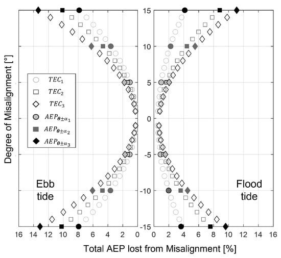
Figure 8.
AEP loss based on flow velocity used , where changed in increments of 1° up to 15° (, and represent 5°, 10° and 15°, respectively). The flood (right) and ebb (left) tide AEP estimates with a clockwise and anti-clockwise shift from the established flow.
Table 5.
AEP percentage loss from misalignment (), where both flood and ebb tidal cycles were analysed for a clockwise and anti-clockwise shift for the three TEC concepts. NOTE is equal to the established flow direction.
Figure 9 shows a time-series of energy captured by TEC for each tide across the measurement campaign, where the lower energy yields are directly related to lower velocities which occur during neap tidal cycles, experienced around periods 12–14 June and 24–26 June. During these periods of lower tidal flow speeds, we see the greatest energy lost due to the modelled misalignment. The amount of energy lost over each tidal cycle varies, but was as high as 3%, 7% and 12% when the TEC is misaligned to the established flow direction by 5°, 10° and 15°, respectively.
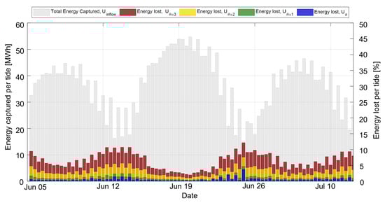
Figure 9.
Energy lost when TEC is misaligned to the flow, where the grey bar is the energy captured per tidal cycle. The blue, green, yellow and red bars represent the energy lost by the TEC facing the established flow , misaligned by (5°), (10°) and (°), respectively.
5. Discussion
This paper demonstrates the importance of accurately estimating the established flow direction to inform tidal developers about TEC orientation and thereby maximise the energy captured. First, it is shown that including data outside of the TECs’ operational limits can skew the established flow direction estimate by up to 4° (see Table 4). The greatest variation in flow direction is found when the tide changes between flood and ebb. The flow velocity and direction evolve over the tidal cycle; removing data beneath the cut-in speed of the TEC will remove the large variations in flow direction and provide a more accurate reference for TEC orientation. In addition, the flow direction can vary up to 13° along the measured water column. The rotor average and PWRA methods are used in this study to capture the variation in the direction along the rotor plane. The results differ by less than 1.2% when comparing the two methods against the averaged hub-height estimate. This work highlights that misalignment between the TEC extraction plane and the flow direction will impact the energy captured. Furthermore, aligning the depth bin from the ADCP to the proposed TEC hub-height when estimating the established flow direction is key, and inaccuracies can impact the amount of energy captured when the TEC orientation is incorrectly informed.
A key objective of this study was to assess the impact on power production when flow data used features misalignment from the TEC extraction plane. The flow direction evolves over a tidal cycle, resulting in the TEC being susceptible to off-axis currents, even when the TEC is aligned to the averaged (over a tidal cycle) flow direction. This is evidenced by the temporal variation in the flow direction, shown in Figure 3 and Figure 4 and the vertical variation displayed in Figure 5. The AEP estimate calculated from assuming the TEC tracks the flow, compared with a fixed TEC heading towards the established flow angle, differed by up to 1%. This is site-specific and will be based on the natural flow direction variation at a tidal site. The variation in the flood tide direction was ≈75°, and whilst the ebb tide direction varied by ≈35° (Figure 6), this resulted in the TEC being off-axis more frequently during the flood tidal cycles; thus, the AEP losses were greater. Furthermore, if the TEC is misaligned with the established flow angle once deployed, the AEP will be overestimated. For a non-yawing TEC, the total AEP loss, as shown in Table 5, can be up to ≈2%, 6% and 13%, when the TEC is incorrectly aligned to the established flow by 5°, 10° and 15°, respectively. This highlights an area of uncertainty when deploying a TEC at a tidal site, as the accuracy of both the TEC heading and flow direction will reduce the uncertainty in the measured power curve and energy yield estimates.
A case study using three horizontal-axis TECs rated at 0.25 MW, 1 MW and 2 MW and occupying the lower, mid and upper regions of the water column, respectively, is presented. The 1 MW machine used real world data as this was available. Figure 5b and Figure 8 show the position of the three TECs and the AEP loss when misaligned to the established flow direction, respectively. Of the three TECs assessed, the 2 MW variant exhibits the greatest AEP losses under misalignment. This is a result of the operational characteristics of the TEC, where the rated velocity is 3.1 m·s, and the flow velocity at the site on a flood tide was 3.2 m·s, whereas the smaller-scale TECs (TEC and TEC) experience more frequent flows in excess of their rated velocity, which mitigates the impact of misalignment. Overall, a tidal energy converter that has a rated velocity beneath the tidal site flow characteristics by ≈10% will operate at full capacity during peak flow conditions even during periods of excessive misalignment up to 25°, at the expense of capturing significantly less energy during times below peak flow conditions. On the other hand, TECs with a rated velocity over or close to the peak flow tidal conditions will suffer significantly if the flow velocity is lower than the rated. This is evident in Figure 9, where the AEP losses are greater under lower flow conditions, commonly referred to as neap cycles. An active yaw mechanism may be most efficient during periods of lower velocity, where the TEC operating characteristics are close to the flow characteristics at the tidal site, to maximise the energy captured and minimise losses.
6. Conclusions
Using methods for data processing that only consider conditions across the turbine during power production will give a more accurate estimate of the established flow direction to inform turbine installation and power performance assessments. The established flow direction estimate used to inform developers about TEC orientation was found to vary by up to 1.2° when using rotor averaging methods and up to 4° when restricting data used to velocities when the turbine is operational.
The performance characteristics of three horizontal-axis tidal turbines manually positioned towards the oncoming flow have been measured relative to a yaw misalignment from the established flow direction. The flow direction naturally evolves over a tidal cycle. When the turbine was aligned to the established flow direction, this caused a difference in energy estimates of up to 1.1% from the theoretical maximum production of a perfectly yawing turbine. When the turbine was misaligned from the established flow direction, the difference in AEP increased. For a 5°, 10° and 15° misalignment, the AEP differed by 2%, 6% and 13% respectively.
The difference between the flow velocity on site and the TEC-rated velocity governs the impact of misalignment on AEP. The observed differences will all have a greater impact when a turbine is rated close to, or above, the maximum flow velocity. Turbines rated beneath the maximum flow velocity at the site by at least 10% will operate at full rated capacity during peak flow conditions even if the TEC is misaligned to the flow direction by up to 25°. Furthermore, the velocity is significantly slower during neap tidal cycles, which is undesirable as it means the turbine is only at an extractable flow velocity for a smaller proportion of the time (further reduced when misaligned to the established flow), reducing the availability of the turbine to generate and capture the extractable resource.
The local bathymetry and channel boundaries differ significantly across different tidal test sites. This work highlights the importance of understanding how the flow direction evolves over a tidal cycle and how this characteristic impacts non-yawing TECs’ performance. Future work can compare and quantify the uncertainty from the variability of the flow direction over a tidal cycle at different sites.
Author Contributions
L.E.: Conceptualisation, Methodology, Formal analysis, Investigation, Writing—original draft, revision. I.A.: Supervision, Writing—review, editing & revision. B.G.S.: Conceptualisation, Methodology, Supervision, Writing—review, editing & revision. All authors have read and agreed to the published version of the manuscript.
Funding
This work was funded as part of the EPSRC, United Kingdom and NERC, United Kingdom Industrial Centre for Doctoral Training in Offshore Renewable Energy (IDCORE), Grant number EP/S023933/1, and sponsored by EMEC.
Data Availability Statement
The datasets used in this research are publicly available at [38].
Acknowledgments
The author would like to thank Mike Partridge (EMEC) and Laibing Jia (Strathclyde) for their support in reviewing the manuscript.
Conflicts of Interest
The authors declare no conflict of interest.
Abbreviations
The following abbreviations are used in this manuscript:
| TEC | Tidal Energy Converter |
| ADCP | Acoustic Doppler Current Profiler |
| PPA | Power Performance Assessment |
| AEP | Annual Energy Production |
| EMEC | European Marine Energy Centre |
| FoW | Fall of Warness |
| ReDAPT | Reliable Data Acquisition Platform for Tidal |
| DE | Equivalent Diameter |
| QC | Quality Control |
| PWRA | Power Weighted Rotor Average |
| RU | Ramp Up |
| WD | Wane Down |
| PF | Peak Flow |
| IEC | International Electrotechnical Commission |
References
- Lewis, M.; Neill, S.P.; Robins, P.E.; Hashemi, M.R. Resource assessment for future generations of tidal-stream energy arrays. Energy 2015, 83, 403–415. [Google Scholar] [CrossRef]
- O’Doherty, T.; O’Doherty, D.M.; Mason-Jones, A. Tidal energy technology. In Wave and Tidal Energy; John Wiley & Sons, Inc.: Hoboken, NJ, USA, 2018; pp. 105–150. [Google Scholar] [CrossRef]
- Sellar, B.; Wakelam, G.; Sutherland, D.R.; Ingram, D.M.; Venugopal, V. Characterisation of tidal flows at the european marine energy centre in the absence of ocean waves. Energies 2018, 11, 176. [Google Scholar] [CrossRef]
- Frost, C. Flow Direction Effects on Tidal Stream Turbines. Ph.D. Thesis, Cardiff University, Cardiff, UK, 2016. [Google Scholar]
- Piano, M.; Neill, S.P.; Lewis, M.J.; Robins, P.E.; Hashemi, M.R.; Davies, A.G.; Ward, S.L.; Roberts, M.J. Tidal stream resource assessment uncertainty due to flow asymmetry and turbine yaw misalignment. Renew. Energy 2017, 114, 1363–1375. [Google Scholar] [CrossRef]
- Harrold, M.; Ouro, P.; O’Doherty, T. Performance assessment of a tidal turbine using two flow references. Renew. Energy 2020, 153, 624–633. [Google Scholar] [CrossRef]
- Harding, S.; Bryden, I. Directionality in prospective Northern UK tidal current energy deployment sites. Renew. Energy 2012, 44, 474–477. [Google Scholar] [CrossRef]
- Paboeuf, S.; Yen Kai Sun, P.; Macadré, L.M.; Malgorn, G. Power performance assessment of the tidal turbine sabella D10 following IEC62600-200. In Proceedings of the International Conference on Offshore Mechanics and Arctic Engineering, Busan, Republic of Korea, 19–24 June 2016; Volume 6. [Google Scholar] [CrossRef]
- EMEC. A List of the Tidal Energy Concepts Known to EMEC. 2020. Available online: https://www.emec.org.uk/marine-energy/tidal-developers (accessed on 21 March 2023).
- Starzmann, R.; Goebel, I.; Jeffcoate, P. Field Performance Testing of a Floating Tidal Energy Platform—Part 1: Power Performance. 2018. Available online: https://tethys-engineering.pnnl.gov/sites/default/files/publications/AWTEC2018-320.pdf (accessed on 21 March 2023).
- MacEnri, J.; Reed, M.; Thiringer, T. Power quality performance of the 1.2 MW tidal energy Converter, SeaGen. In Proceedings of the ASME 2011 30th International Conference on Ocean, Offshore and Arctic Engineering, Rotterdam, The Netherlands, 19–24 June 2011. [Google Scholar] [CrossRef]
- Ocean Energy Systems. Tidal Current Energy Developments Highlights from the OES. 2021. Available online: https://www.ocean-energy-systems.org/publications/oes-brochures/document/tidal-current-energy-developments-highlights/ (accessed on 21 March 2023).
- Qian, P.; Feng, B.; Liu, H.; Tian, X.; Si, Y.; Zhang, D. Review on configuration and control methods of tidal current turbines. Renew. Sustain. Energy Rev. 2019, 108, 125–139. [Google Scholar] [CrossRef]
- Sutherland, D.; Sellar, B.; Harding, S.; Bryden, I. Initial flow characterisation utilising turbine and seabed installed acoustic sensor arrays. In Proceedings of the European Wave and Tidal Energy Conference, Aalborg, Denmark, 2–5 September 2013. [Google Scholar]
- Mcnaughton, J.; Sinclair, R.; Sellar, B. Measuring and modelling the power curve of a commercial-scale tidal turbine. In Proceedings of the 11th European Wave and Tidal Energy Conference, Nantes, France, 6–11 September 2015. [Google Scholar]
- Divett, T.; Vennell, R.; Stevens, C. Maximising Energy Capture by Fixed Orientation Tidal Stream Turbines in Time-Varying off Axis Current. 2009. Available online: https://www.academia.edu/963239/Maximising_energy_capture_by_fixed_orientation_tidal_stream_turbines_in_time_varying_off_axis_current (accessed on 21 March 2023).
- Stanton, B.R.; Goring, D.G.; Bell, R.G. Observed and modelled tidal currents in the New Zealand region. N. Z. J. Mar. Freshw. Res. 2001, 35, 397–415. [Google Scholar] [CrossRef]
- PD IEC/TS 62600-200; 2013 BSI Standards Publication Marine Energy—Wave, Tidal and Other Water Current Converters Energy Converters—Power Performance. International Electrotechnical Commission (IEC): Geneva, Switzerland, 2013.
- Mcnaughton, J.; Sinclair, R.; Harper, S.; Dobson, D.P.; Chesman, P. ReDAPT: Initial Operation Power Curve (MC7.1). Energy Technologies Institute, 2014. Available online: https://ukerc.rl.ac.uk/ETI/PUBLICATIONS/MRN_MA1001_1.pdf (accessed on 21 March 2023).
- EMEC. The Worlds First International Power Performance Assessment by EMEC for Verdant Power. 2021. Available online: https://www.emec.org.uk/about-us/our-tidal-clients/verdant-power (accessed on 21 March 2023).
- Clayton, R. Quantifying and Reducing Uncertainty in Tidal Energy Yield Assessments. Ph.D. Thesis, University of Exeter, Exeter, UK, 2020. [Google Scholar]
- Sellar, B.; Sutherland, D.R. Tidal Energy Site Characterisation at the Fall of Warness, EMEC, UK Energy Technologies Institute (ETI) ReDAPT MA1001 (MD3.8 Release v4.0). Technical Report. 2016. Available online: http://redapt.eng.ed.ac.uk (accessed on 21 March 2023).
- Waggitt, J.J.; Cazenave, P.W.; Torres, R.; Williamson, B.J.; Scott, B.E. Predictable hydrodynamic conditions explain temporal variations in the density of benthic foraging seabirds in a tidal stream environment. Proc. Ices J. Mar. Sci. 2016, 73, 2677–2686. [Google Scholar] [CrossRef]
- Polagye, B.; Thomson, J. Tidal energy resource characterization: Methodology and field study in Admiralty Inlet, Puget Sound, WA (USA). Proc. Inst. Mech. Eng. Part A J. Power Energy 2013, 227, 352–367. [Google Scholar] [CrossRef]
- Galloway, P.W.; Myers, L.E.; Bahaj, A.S. Experimental and numerical results of rotor power and thrust of a tidal turbine operating at yaw and in waves. In Proceedings of the World Renewable Energy Congress—Sweden, Linköping, Sweden, 8–13 May 2011; Linköping University Electronic Press: Linköping, Sweden, 2011; Volume 57, pp. 2246–2253. [Google Scholar] [CrossRef]
- Lewis, M.J.; Neill, S.P.; Hashemi, M.R.; Reza, M. Realistic wave conditions and their influence on quantifying the tidal stream energy resource. Proc. Appl. Energy 2014, 136, 495–508. [Google Scholar] [CrossRef]
- Blackmore, T.; Myers, L.E.; Bahaj, A.S. Effects of turbulence on tidal turbines: Implications to performance, blade loads, and condition monitoring. Int. J. Mar. Energy 2016, 14, 1–26. [Google Scholar] [CrossRef]
- Galloway, P.W.; Myers, L.E.; Bahaj, A.S. Quantifying wave and yaw effects on a scale tidal stream turbine. Renew. Energy 2014, 63, 297–307. [Google Scholar] [CrossRef]
- Perez, L.; Cossu, R.; Grinham, A.; Penesis, I. An investigation of tidal turbine performance and loads under various turbulence conditions using Blade Element Momentum theory and high-frequency field data acquired in two prospective tidal energy sites in Australia. Renew. Energy 2022, 201, 928–937. [Google Scholar] [CrossRef]
- Sutherland, D.R.J. Assessment of Mid-Depth Arrays of Single Beam Acoustic Doppler Velocity Sensors to Characterise Tidal Energy Sites. Ph.D. Thesis, The University of Edinburgh, Edinburgh, UK, 2015. [Google Scholar]
- Osalusi, E.; Side, J.; Harris, R. Structure of turbulent flow in EMEC’s tidal energy test site. Int. Commun. Heat Mass Transf. 2009, 36, 422–431. [Google Scholar] [CrossRef]
- European Commission. RealTide: Advanced monitoring, simulation and control of tidal devices in unsteady, highly turbulent realistic tide environments. In H2020 Programme for Research and Innovation; European Commission: Brussels, Belgium, 2019; pp. 1–45. [Google Scholar]
- IOOS. Manual for Real-Time Quality Control of Stream Flow Observations (Qartod) v2.1. 2019. Available online: https://repository.library.noaa.gov/view/noaa/21151 (accessed on 21 March 2023). [CrossRef]
- RDI. Acoustic Doppler Current Profiler: Principles of Operation, a Practical Primer. P/N 951-6069-00; Teledyne RD Instruments: Poway, CA, USA, 2011; p. 56. [Google Scholar]
- RDI. RD Instruments Acoustic Doppler Current Profilers Application Note ADCP Beam Clearance Area. Application Note. 2002. Available online: https://doczz.net/doc/7906577/adcp-beam-clearance-area—sf (accessed on 21 March 2023).
- Sellar, B.; Old, C.; McCallum, P. RealTide Technical Report, D2.2-Next Generation Flow Measurements and Flow Classification. Technical Report. 2021. Available online: https://www.realtide.eu/ (accessed on 21 March 2023).
- FASTWATER: Freely Available Simulation Toolset for Waves, Tides and Eddy Replication: Open Software Repository. 2022. Available online: https://git.ecdf.ed.ac.uk/uoe-ies-open-tools/fastwater (accessed on 21 March 2023).
- Sellar, B.; Old, C.; Ingram, D. Dataset: Field-Measurements Aligned to the Implementation of a Tidal Energy Converter’s Power Performance Assessment (IEC 62600-200 PPA Type B); DataShare. 2022. Available online: https://datashare.ed.ac.uk/handle/10283/4423 (accessed on 21 March 2023).
Disclaimer/Publisher’s Note: The statements, opinions and data contained in all publications are solely those of the individual author(s) and contributor(s) and not of MDPI and/or the editor(s). MDPI and/or the editor(s) disclaim responsibility for any injury to people or property resulting from any ideas, methods, instructions or products referred to in the content. |
© 2023 by the authors. Licensee MDPI, Basel, Switzerland. This article is an open access article distributed under the terms and conditions of the Creative Commons Attribution (CC BY) license (https://creativecommons.org/licenses/by/4.0/).