Review

Review of Hysteresis Models for Magnetic Materials

Division of Electricity, Department of Electrical Engineering, Uppsala University, 75121 Uppsala, Sweden
*
Author to whom correspondence should be addressed.
Energies 2023, 16(9), 3908; https://doi.org/10.3390/en16093908
Submission received: 6 March 2023 / Revised: 11 April 2023 / Accepted: 15 April 2023 / Published: 5 May 2023

Abstract

:
There are several models for magnetic hysteresis. Their key purposes are to model magnetization curves with a history dependence to achieve hysteresis cycles without a frequency dependence. There are different approaches to handling history dependence. The two main categories are Duhem-type models and Preisach-type models. Duhem models handle it via a simple directional dependence on the flux rate, without a proper memory. While the Preisach type model handles it via memory of the point where the direction of the flux rate is changed. The most common Duhem model is the phenomenological Jiles–Atherton model, with examples of other models including the Coleman–Hodgdon model and the Tellinen model. Examples of Preisach type models are the classical Preisach model and the Prandtl–Ishlinskii model, although there are also many other models with adoptions of a similar history dependence. Hysteresis is by definition rate-independent, and thereby not dependent on the speed of the alternating flux density. An additional rate dependence is still important and often included in many dynamic hysteresis models. The Chua model is common for modeling non-linear dynamic magnetization curves; however, it does not define classical hysteresis. Other similar adoptions also exist that combine hysteresis modeling with eddy current modeling, similar to how frequency dependence is included in core loss modeling. Most models are made for scalar values of alternating fields, but there are also several models with vector generalizations that also consider three-dimensional directions.

1. Introduction

Laminated magnetic cores are based on the magnetizing of alternating fields which experience hysteresis. In this phenomenon, the magnetization is not just a function of an applied field, but also dependent on the history of the previous states of magnetizations. It is usually seen as loops in the magnetization curve for one cycle of the applied magnetic field strength. Where the trajectory of the demagnetizing is different from the one while magnetizing.
General reviews on hysteresis models of magnetization can be read in works by Jiles [1,2], Liorzou et al. [3], Andrei [4], Cardelli [5] and Bavendiek [6]. The works of Takach and Lauritzen [7] and Petrun et al. [8] provide more specific information for soft magnetic iron cores, and similarly also for hysteresis energy losses by Steentjes et al. [9].
This article is structured by first describing Duhem models, such as the Coleman–Hodgdon model and the Jiles–Atherton model, in addition to the Tellinen model and others. Subsequently, history-dependent models based on series of reversal points, such as the Preisach model and the Play model, are presented. Their history dependence could be described as a series of reversal points.
Some models are based on adopting curve shapes from the major loop for approximating reversal curves within the hysteresis area, such as models by Talukdar–Bailey and Tellinen, usually by downscaling the curve to fit a minor loop curve. Such models are adopted both for Duhem type models and for Madelung’s rules with history dependence.
The last section describes models that consider rate-dependency and frequency dependence, such as models linked to iron losses with eddy currents. Furthermore, the Chua model, which is not a hysteresis model in itself, but modelling similar phenomena such as nonlinear magnetization curves and nonlinear eddy currents, is described.

2. What Is Hysteresis?

The word hysteresis was coined by the physicist Ewing more than 100 years ago [10,11,12]. It was intended as a name for the phenomenon itself, so it could be discussed without focus on the different theories about its cause [10]. The expression differentiates hysteresis from loops that are caused by dynamic effects, such as viscosity and eddy currents.
Hysteresis has, among others, two main features; memory and branching (see Figure 1). Even if a system does not depend on previous states and position, it has at least “local memory” where all information is given by the present position and their directions [13]. The essence of the hysteresis is branching, describing the existence of alternative trajectories depending on the direction of how the field alternates [14]. This is associated with rate-independence, that it is dependent on the direction of change, but not on the rate of the change. It is, however, hard to find a general definition for hysteresis that covers all areas. Hysteresis is characterized by multiple stable equilibriums and dynamics faster than the input [12]. A curve without hysteresis is on the contrary called an anhysteretis curve.

2.1. Rate-Independency and Rate-Dependency

Hysteresis should not be confused with loops that occur in phase-portraits of systems with a phase shift or phase-lag between sinusoidal inputs and outputs [13], such as electrical AC circuits with complex valued impedances. The loop in these kinds of systems are then just a consequence of the phase angle in the dynamic system. Hysteresis, on the contrary, is a phenomenon that would remain even without dynamic effects, that is without time-lags and phase-shifts [15]. Hysteresis is rate-independent, while these effects are rate-dependent [16].
Ewing [10] coined the term hysteresis phenomenon in order to move the phenomenon away from the different physical explanations, although he still states that this “frictional resistance” resembles the friction of solid objects, rather than the viscosity of liquids. Because hysteresis is independent of speed, while viscosity is dependent on the speed.
Here, we can see a separation between the more friction-like part, which is rate-independent, and the more viscosity-like part, which is rate-dependent. The viscosity in this case is the eddy currents, and the friction is instead magnetic hysteresis. Even if these two phenomena may be treated separately, they are often combined in several hysteresis models. These use to be called rate-dependent hysteresis model or dynamic hysteresis models. Rate-independent models are then referred to static hysteresis models.
Although hysteresis models are generally rate-independent models, there are also rate-dependent hysteresis models that also consider a frequency dependence [17,18]. As such, these models consider both rate-independency and rate-dependence, similar to mechanical systems that consider both friction and viscosity.

2.2. Phenomenological or Physical Models?

There is a difference between phenomenological models and physical models [19]. The differences are in whether the model only describes the curve shapes of the hysteresis phenomenon, or if they also explain the physics behind the phenomenon. Where phenomenological models are based on mathematics and curve fitting, separated from those that actually are based on physics and physical reasoning [20]. Another way to refer to the phenomenological models is mathematical models [21]. This is a term that can also cover the fact that there still is a lot of mathematics developed for phenomenological models, such as the Preisach model.
The Jiles–Atherton model, the Coleman–Hodgdon model and the Preisach model can be seen as phenomenological in contrast to Micromagnetic models and the Stoner–Wohlfarth model that are physical [4]. Micromagnetic modelling is instead modeling of the domain behavior [22,23]. This is often put in contrast to Preisach models that are based on measurements and characterization of materials, but without the link to physics that micromagnetic bears [20,24]. The Preisach model is mostly referred to as a phenomenological model [25,26,27,28,29,30]. However, it could also be linked to statistical mechanics since it is based on the way of seeing it as built by several consisting parts [31], such as models where the Preisach model is adopted with pseudo-particles based on physical models [32].
The Jiles–Atherton model employs functions and parameters based on physics [25,26,33,34,35]. However, the parameters are obtained by phenomenological methods [36,37,38], such that the model is considered a phenomenological model [6,36,39,40,41,42].

3. History Dependence and Independence

Another categorization is between history-dependent and -independent models [40]. Most algebraic and differential models are history-independent models, such as Duhem models and transplantation type models. The memory in history-independent models use to be the present position B , H and the directions. The directions are usually expressed as a rate-independency s i g n ( d H / d t ) , but can also be seen as the change relative to the previous position s i g n ( M M 0 ) or as the direction of input variable | d x | / d x . The differential models used to be based around solving d B / d H or similar with B, H or M. The transplantation type models are built on approximating unknown hysteresis curves from a known major loop curve.
History-dependent models are instead often constructed as sum and integrals based on differential distributions. These can be built on using equations between predefined points, given by a history of reversal points. One such model is the Preisach model.
Some differential models are based on modelling hysteresis by viscosity or eddy currents, i.e., by solving d B / d t . They are then not proper hysteresis models, since the loop is caused by a phase lag rather than a proper hysteresis. One advantage may instead be the inclusion of rate-dependency, which means that they are frequency dependent.

3.1. History Dependency

History dependency means that the hysteresis models are not just dependent on the present input, but are also dependent on the history. This means that it is not a simple function of the input variable [17,18]. It can be expressed as:
B ( H ) = B ( H ( t ) , History )
The history dependence could be expressed as [43,44]:
B ( H ) = B ( H ( t ) , H g )
With the history H g = { H ( t w ) } depending on the previous time t w < t [43,44,45]. Considering all previous time since the initial time t 0 , starting from initial magnetization B ( 0 ) .
The time variable is usually not important in this context of history dependence. This means that the history dependence is instead appearing through the present state of the magnetization. Either by the present state of the output variable (i.e., B), or by a distribution of several underlying components as in the Preisach model.

3.2. History Independency

While history-dependent models depend on all previous positions of the system, other types of hysteresis models could be history independent. The name might suggest that they lack memory, but as with all hysteresis models the models still have a dependency previous path [46]. The memory is just constructed in more simple way, often referred to as the “local memory approach” [13,47]. History-dependent models are then referred to as a “non local” [13] or “global memory approach” [47]. History independence has a simplified memory reduced to the information through the present position ( B , H ) and the speed rate d H / d t . An important category among these are the rate-independent models that are called Duhem models [45]. With the history H t expressed only by the local history, from the position B ( t ) and the direction s i g n ( d H ( t ) / d t ) , as in:
B ( H ) = B ( H ( t ) , B ( t ) , sign d H ( t ) d t )
This limited dependence on the past have consequences for the trajectory. In Duhem models there is a phenomenon called “drifting” that presents a problem when modelling asymmetric minor loops. The lack of return point memory results in unrestricted trajectories for periodic input signals. The advantage of history dependency is then that they give minor loops that do not drift away for each repeated loop. Because the previous trajectories are not saved, all curves point towards the major loop [40].
History-independent models always have drifting for non-concentric asymmetric loops, while most history-dependent models do not have this problem. Still, an incorrect construction of a history-dependent model can still lead to drifting, such as history-dependent models that lack a proper return point memory, so that it fails to generate closed minor loops (further explained in later sections).
Drifting was analyzed in hysteresis models by Krasnoselskii and Pokrovskii [48] via a concept called “vibro-correctness”, detailing that a small variation in the input cycling only will cause small variations in the output cycling.

3.3. Other Types of History Dependency

There are also some models that have special history dependencies that may not easily be placed in any category. These are models that neither store the complete history nor just limit the history to the present position.
One such model is the model by de Almeida [49], which also depends on the last reversal point ( H r , B r ). The model creates an arctan-function between the reversal point and the saturation point [49]. A similar process is employed in the model by Hauser [50,51,52].
An alternative would be to instead store the last reversal point for return point memory, to give closed minor loops. However, the return point memory of Madelung’s rules is not always desired, because it is not an entirely correct model of actual trajectories.
Alternative methods that include accommodation were developed in several studies [53,54,55,56].

4. Algebraic, Differential and Integral Models

One way of categorizing is based on distinguishing whether they are algebraic equations, differential equations or integral equations [57,58,59]. Some examples of differential models include the Jiles–Atherton model and Coleman–Hodgdon model, which are expressed as differential equations. Furthermore, an example of an integral model is the Preisach model, which usually is based on solving an integral expression.
These categories may at first seem to be clear to separate, but could result in unclear distinctions between the categories. An algebraic equation could be a solution to a differential equation, and algebraic equations could be expressed as differential equations. Differential equations are usually solved with integrals and integral equations could be based on distributions in a differential form.
Some phenomenological models (such as the Talukdar–Bailey model) are based on scaled curve shapes. These could either be expressed by an algebraic expression or as a differential equation. The Preisach model is solved based on an integral, but could integrate a differential expression.

5. Duhem Models

A common term for several differential equation models is to refer to them as “Duhem model”, based on the models that are used by Duhem [60,61,62,63,64], mostly used for hysteresis in mechanical deformation of materials. However, this is also applied to magnetism. Duhem [60] links hysteresis to irreversible energy losses in contrast to reversible energy that is stored as thermodynamic potential.
The models are usually expressed in the form of a differential equation. Where a useful criteria for such a model is that the loop should be obtainable for any initial point, any amplitude and any oscillatory change in H [65].
The models create a directional dependence, so that there are different functions depending on the direction, as seen in Figure 2.
All Duhem models are rate-independent models, meaning that they depend on the direction of the input, but not the rate of the input. This is expressed by the dependency on s i g n ( d H / d t ) for d B / d H . Furthermore, for Duhem models the function d B / d H is rate-independent. This can be seen by separating it in products:
d B d t = d B d H d H d t
There are, however, writers who describe them as rate-dependent models, because d B / d t is dependent on d H / d t [59]. This is not the common way of seeing rate-dependency, because rate-independency use to be defined based on the definition of d B / d H . Rate-dependency is different in such a way that the size of the hysteresis loop will depend on the input speed d B / d H . In Duhem models, there is no dependence on the rate of the speed for a hysteresis loop.
The derivative d B / d H corresponds to the permeability, which is never negative for ferromagnetic and ferrimagnetic materials. So, an increasing H gives an increasing B, and a decreasing H gives decreasing B [16,48,57].

5.1. Increasing and Decreasing Curves

These can be categorized into two families of curves, depending on the directions, as either increasing or decreasing. It is conveniently expressed as a differential Equation [16,45]:
d B d H = f ( B , H , sign d H d t )
The main feature of Duhem models is that there are two groups of functions depending on the direction, and that the slope and trajectory depends on the position ( B , H ) [16]
d B d H = f d ( B , H )   if   d H / d t < 0 f i ( B , H )   if   d H / d t > 0
It can also be written as increasing curves and decreasing curves
B = F d ( B , H ) if   d H / d t < 0 F i ( B , H ) if   d H / d t > 0
There are then two different curve paths of B depending on the direction of the change in H. Suitably implemented with a symmetry of the curves given by [65]
f i ( B , H ) = f d ( B , H )
So that a hysteresis cycle acts symmetrically between increasing and decreasing curves.

5.2. Classical Approach to Duhem Models

The classical Duhem models are written with two separate terms, one reversible and the other irreversible. For mechanical systems, the slope is separated as two different types of stiffnesses. That is as one reversible elastic stiffness, and one irreversible hysteresis stiffness [17,18]. For magnetism, it separates between an ideal soft magnetic permeability, and hysteresis properties. With one contribution from reversible magnetization and demagnetization, and another from irreversible demagnetization and magnetization. That is on the form:
d B d H = f r e v ( H ) ± f i r r ( H , B )
The function f r e v represents the ideal soft magnetic materials which would be without coercive magnetic properties. The function f i r r is introduced to represent materials with coercivity and remanence, which introduces the function of hysteresis.
Duhem [60] also introduces two criteria for the functions, first of symmetry in reversible component, as in:
f r e v ( B , T ) = f r e v ( B , T )
Furthermore, another type of symmetry for the irreversible part:
f i r r ( B , H , T ) = f i r r ( B , H , T )

5.3. Anhysteresis Curve and Limiting Boundaries

The increasing and decreasing curves ( F i and F d ) are limited by an upper and lower bound C u and C l , as illustrated in Figure 3. Such that the upper and the lower limiting curves are the outermost curves [17,18,58]. These boundaries are then located at the greatest hysteresis width. In the case of magnetism, it is related to the major loop curves, which is the greatest possible hysteresis loop.
One interesting curve in Duhem models is the Anhysteresis function, which is used to set the shape of the magnetization curve when hysteresis is excluded. A similar function was discussed by Duhem, but they referred to as a curve of “natural states” [60]. The boundaries C u and C l can be expressed related to the anhysterestic curve C a , based on a hysteresis difference C h (as seen in Figure 4). Similar to the structure of separating the function into a hysteresic part and anhysteretic part, as in models studied by Sequenz [66], Rivas [67] and Battistelli [68]. Then, with:
B ( H ) = C u = C a + C h if   d H / d t < 0 C l = C a C h if   d H / d t > 0
where the anhysteretic C a and hysteretic C h are given by the major loop by two functions as
C a = ( C u + C l ) / 2 C h = ( C u C l ) / 2

5.4. Examples of Duhem Models

There are several models of magnetic hysteresis that are Duhem models, with the two most common ones being the Coleman–Hodgdon model [69,70,71] and the Jiles–Atherton model [72,73], also existing in several modified versions, and in inverse forms. An early model is also the Cisotti model [74,75,76]. However, it has also been studied for magnetism in a general way as Duhem models, without referring to any specific type [45,77,78,79,80,81,82,83].
It is, however, not always referred to as the Duhem model. The model by Takagi for magnetism [65,84], or for mechanics by Babuška [85,86,87,88,89,90]. The Duhem model is sometimes also referred to as “Madelung model” [44,48,91,92]. However, Madelung’s model does not have the same history dependence [90,93]. Madelung’s model is more similar to Prandtl’s model [94], but based on adoptions with magnetic functions by Gans [95].
Some Duhem models in other subjects are the Dahl model of friction [96,97,98], and its modification into the LuGre model [99,100], and the similar Bouc–Wen model [89,101,102,103]. The model can be modified to represent different rate-independent systems [58]. Even if it usually not used for magnetism, the Bouc–Wen model has been applied to model magnetism by Laudani et al. [104].

5.5. The Model in Duhem’s Work

Duhem [60] use an adoption of Clausius inequality, which could be rewritten for a magnetic field strength, H and a flux density, B. A change in the magnetostatic energy H d B minus a change in the Helmholz free energy F will not be equal to zero, because of hysteresis losses. Note that Duhem writes the expression for a magnetization M ( H ) , while the adoption here is for the flux density B ( H ) . However, the same method could easily be rewritten for flux densities by adding the field together with the field H as B = μ 0 ( M + H ) . For flux density, it is expressed as
H d F d B d B > 0
The difference between the stored energy and the applied change in energy is modeled by the irreversible function f i r r .
Duhem’s model [60] describes that a change in magnetic field strength, d H will be dependent on changes in d B and d T , but also on the absolute value of the change in magnetic field strength | d B | . That is:
d H = d 2 F ( B , T ) d B 2 d B d 2 F ( B , T ) d B d T d T + f i r r ( B , H , T ) | d B |
It can now be considered that we obtain the special ratio of | d B | / d B as s i g n ( d B ) = ± 1 . Which provides the fundament of the rate-independency, because it corresponds to s i g n ( d B / d t ) for d t > 0 . The Duhem model is then simplified as:
d H = d 2 F d B 2 ± f i r r d B + d 2 F d B d T d T
Which with neglected temperature dependence is
d H d B = d 2 F d B 2 ± f i r r ( M , H )
Written instead in notation based on Maxwell relations as
d H = d H d B T d B + d H d T B d T
The magnetic field strength could be seen as a combined field H = H r e v + H i r r . When including hysteresis expressed as a sum by an irreversible part H i r r , together with the reversible part H r e v as:
d H = d H r e v d B T d B + d H i r r d B T | d B | + d H d T B d T
With the irreversible part as
d H i r r d B = f i r r
Furthermore, the reversible part as
d H r e v d B = f r e v
The model is further simplified if the temperature dependency is neglected [60], as in:
d H d B T = f r e v ( T , M ) + f i r r ( H , B , T ) | d B | d B

5.6. Linked to Energy Losses

The equivalence in magnetization would be to split the magnetic energy density w into a reversible and irreversible part, which corresponds to the stored magnetic energy w S and the hysteresis energy losses, w L , respectively:
B 1 B 2 H · d B = w S + w L
The approach to the energy losses in Duhem’s model is based on irreversible losses w ( B , H , T ) , expressed with a localization in the B , H -plane. The irreversible energy dissipation could be linked to area in the magnetizing curve ( B , H -curve) [105,106,107]. Expressing the iron losses for a cycle of a periodic magnetic alternation
H · d B = w L
By differentiating, in analogy of Duhem, we get an equation for the reluctivity as:
d H d B = d 2 w S d B 2 f r e v ( B ) ± d 2 w L d B 2 f i r r ( B , H )
The slope in expressed by the equation is on the form of a reluctivity, for the combined field
H ( B ) = H r e v ( B ) ± H i r r ( B , H )

5.7. Coenergy Expression

Equations on the form H ( B ) are generally seen as an “inverse” form, since the form B ( H ) is the most common expression. It could then be convenient to introduce a magnetic flux density written on the form
B ( H ) = B r e v ( H ) ± B i r r ( H , B )
An adoption of the Duhem model then becomes:
d B d H = d B r e v d H ± d B i r r d H
This will have a clear impact on the Duhem model, and its link to energy. It would allow the model to represent a system of coenergies, instead of energies. This is now redone by writing the energy density by Gibb’s free energy
d B = d 2 G ( H , T ) d H 2 d H + f i r r ( B , H , T ) | d H |
The inverse expression H ( B ) is now seen to have an advantage in its direct link to the expression of the energy. However, the common use of the form B ( H ) is still easy to understand, since it conveniently describes how the induced flux density B is for an applied field strength H.

6. Coleman–Hodgdon Model

The Coleman–Hodgdon Model or Hodgdon model was developed in the 1980s for hysteresis in soft magnetic materials [69,70,71,108]. They are also sometimes referred to as synonymous to Duhem models [59,109,110,111].
The model is generally written as:
d B d t = α c ( f ( H ) B ) d H d t + g ( H ) d H d t
Based on the two functions f ( H ) and g ( H ) , and a parameter α c which could differ between different adoptions of the model. The anhysteretic curve f ( H ) describes the shape of the hysteresis, and the reversible function g ( H ) describes the tendency for drifting from the anhysteresis curve. The hysteresis is then set by the parameter α c . The complexity of the functions f ( H ) and g ( H ) varies, depending on the model of the implementation. They are usually chosen specifically for as material to fit experimental data. Some examples of functions are illustrated in Figure 5 [112,113].
Or also rewritten, so that the rate-independency can be made clearer, by canceling d H / d t , as in:
d B d H = g ( H ) + α c ( f ( H ) B ) sign d H d t
Alternatively written with a ±-sign, for the sign-function, by
d B d H = g ( H ) ± α c ( f ( H ) B )
The first term g ( H ) is the reversible term and could be seen as similar to the derivative of the anhysteresis function f ( H ) . That is
g ( H ) d f ( H ) d H
The function g ( H ) also has a role to define how the slope d B / d H drifts away from the anhysteresis function f ( H ) , and setting the initial curve. It is then preferably lower than d f ( H ) / d H , such that
g ( H ) < d f ( H ) d H
Otherwise, it will remain along the anhysteresis curve, and then move without hysteresis.
The second term describes how the slope depends on the distance x to the anhysteresis, where we can write the distance as
x = f ( H ) B
The slope d B / d H increases based on a parameter α c . So that an increased distance increases the slope, by α c x . When the distance x is high enough, the slope d B / d H will follow the slope of the anhysteresis curve and the distance will cease to increase.
This can be expressed by the derivative of the distance
d x d H = d f ( H ) d H d B d H
This can be expressed by two limiting curves, where the limiting curves are the maximum distances that the hysteresis model has relative to the anhysteresis function. With one upper boundary for the outermost decreasing curve, and one lower boundary for the outermost increasing curve. These limits then act similar to the curves of the major loop, which is the greatest possible hysteresis loop. With a decreasing derivative of the distance, d x / d H , for increasing distances x relative the anhysteresis function, as shown in Figure 6, (defined to be inside the major loop).
The second term α c x could also be modified with other functions. Such as rewriting the linear function α c x as any other function α ( B ) [114,115].
The irreversible function f i r r in Duhem’s model, is different from the function f in the Coleman–Hodgdon model. The irreversible part in the case of the Coleman–Hodgdon model is the term
d B i r r d H = α c ( f ( H ) B ) = α c x ( B )
and the reversible part is the function g ( H )
d B r e v d H = g ( H )
where the reversible function g ( H ) usually is chosen in shape that resembles the derivate of anhysteresis function f ( H ) .

Inverse Coleman–Hodgdon Model

The model is written for the common form of solving B ( H ) in the B , H -plane, but is inverted relative the model in Duhem’s work. There is also an inverted version of the Coleman–Hodgdon model, developed by Hodgdon [71]. It more resembles the structure of Duhem’s model based on energies, and has then a better link to energy density and magnetization loss modelling. The model is written as
d H d t = α c ( f ( B ) H ) d B d t + g ( B , d B / d t ) d B d t
canceling d B / d t in the equation, it becomes
d H d B = g ( B ) + α c ( f ( B ) H ) sign d H d t
Furthermore, written as
d H d B = g ( B ) ± α c ( f ( B ) H )
Compared to the other model it defines another distance x, defined in the H-direction, as
x = f ( B ) H

7. Jiles–Atherton Model

One of the most frequently applied and cited hysteresis models is the Jiles–Atherton model, which was developed in the 1980s [72,73]. It is constructed in a way that makes it into a typical Duhem hysteresis model, with a reversible part that acts as an anhysteresis curve and an irreversible part that includes the impact of hysteresis. The model is wide spread, and is relatively simple to apply, both since it uses few parameters and does not require any advanced history dependence.
It is mainly used for soft magnetic materials for laminated steel cores, but has also been adopted for permanent magnet materials [116], such as NdFeB [117,118] and isotropic NdFeB [119]. The model is used together with many different software programs for simulation and FEM [120,121]. Furthermore, it has been included in both Comsol and Spice [122,123], and been used with Ansys [124]. The model has also been adopted for a relation between magnetic flux and current, to link it to circuit analysis and power system analysis [125].
The model is constructed as a differential equation as
d M d H = 1 1 + c d M i r r d H + c 1 + c d M a n d H
Based on the anhysteresis function
M a n = M s ( coth H e a a H e ) with H e = H + α M
The magnetization M in the model could then be obtained by solving the differential equation:
d M d H = 1 1 + c δ d M a n M k δ α ( M a n M ) + c 1 + c d M a n d H
The Jiles–Atherton model is based on magnetization, M ( H ) instead of flux density, B ( H ) , but could be rewritten for flux density by simply considering B = μ 0 ( M + H ) .
It mainly consists of five parameters, given by Table 1 [126].
The two other parameters of the functions are δ and δ d . The parameter δ = s i g n ( d H / d t ) accounts for the directional dependency, linked to the rate-independency of Duhem models, and δ d as introduced by Deane [127] to compensate for some minor problems with an unphysical negative permeability in the original model. There is, however, still a risk of negative permeability, as addressed by Padilha [128].
The model is based on a clear set of parameters, compared to many other models, such as the Coleman–Hodgdon model or the Preisach model, that does not specifically state the curve shape or distribution function. Still, it is not obvious how the parameters should be found for the Jiles–Atherton model, and there are several studies that introduce methods for parameter estimation [34,129,130,131,132,133,134,135]. There are methods on how to find the parameters in the model. The work to acquire the parameters could be complicated, but since the method is so wide spread it could be easy to find parameters based on various previous studies based on previous measurements.
The hysteresis part of the model is based on modelling pinning of domain walls.

7.1. Phenomenological Anhysteresis Function

The model is physically based, but the physicality has been criticized. Several studies refer to the Jiles–Atherton model as a phenomenological model [136]. Some authors have criticized that the method is based on coenergy rather than energy, and that it does not reproduce precise curve shapes [137]. However, another question is also how it uses physical functions in a phenomenological application for the anhysteresis function, which acts as the backbone of the model.
The anhysteresis function is based on the Langevin function,
L ( x a ) = coth ( x a ) 1 x a
which was originally used for describing the physics of temperature dependence of a magnetization. Its adoption in the Jiles–Atherton model is, on the contrary, entirely phenomenological [138], where it only applies the same curve shape as the Langevin function, but with parameters with an entirely other approach than the classical Langevin function. Written as
x a = H e a
It also exists adopted in other similar versions [9,139]. Since it only uses the curve of the function, it could alternatively be improved by any other curve that could fit. One simple alternative to the anhysteresis functionis is the similar t a n h ( H ) function, proposed by Takacs [138,140]. However, many other anhysteresis functions has been studied, such as the Gaussian error function, exponential functions or functions based on square-roots [141,142]. Other modifications could instead focused on the pinning driven hysteresis, to adopt the initial curve to resemble the Rayleigh model [143,144,145]. The model is quite similar to the Coleman–Hodgdon model, and could be simplified by a similar approach to the Coleman–Hodgdon model, as by Carpenter [146].
The parameter a usually sets the temperature dependence of the physical Langevin function, based on the magnetic moments and the energy of heat [5,72,73]. However, the parameter a is here only treated as a shape parameter for the curve fitting of the anhysteresis function. Since the parameter a is phenomenological, it can be changed to any other function based on curve fitting. An improved temperature dependence of the function would instead be included as a temperature dependence (T) of the saturation magnetization, that is as M s ( T ) [141,147,148], or allowing the parameters to be different depending on the temperature [147,149,150].
Another part of the anhystereisis function that is also a phenomenological adoption is the effective field,
H e = H + α M
and also includes a dependence on the magnetization. The equation for the effective field is written similar to Weiss’ molecular field α M , but without the same physical meaning. It is here used as a parameter for curve fitting. This also opens up for adoptions of other functions for the effective field [142]. Other approaches to improve the physicality of the effective field have been to include for instance the impact of the demagnetizing field [151].
Nevertheless, the Langevin function has shown to be a simple and efficient way of generating anhysteresis functions with a phenomenologically correct curve shape. Since it has the characteristic S-shape of a magnetization curve, that could be modified by choosing different parameters.

7.2. Illustrating That It Is a Duhem Model

Jiles–Atherton model is defined for a magnetization M, and we can easily rewrite it related to flux density B as
d B d H = μ 0 d M d H + 1
The hysteresis part of Jiles–Atherton model depends on the distance x = M M a n , similar to the Coleman–Hodgdon model, but with another function for the dependence. The irreversible term of the Duhem model ( d B i r r / d H = μ 0 d M i r r / d H ) is
d M i r r d H = 1 1 + c x ± k α x
The reversible part is lower than the slope of the anhysteresis curve M a n , since it is decreased by the parameter c such that the reversible term ( d B r e v / d H = μ 0 ( d M r e v / d H + 1 ) ) is
d M r e v d H = c 1 + c d M a n d H

7.3. Anisotropic Versions of the Models

Jiles–Atherton model with adoptions for considering material anisotropy by tensor adoption of pinning in the vector model by Bergqvist [152], followed by modifying the hysteresis. However, also, by modifications on the anhysteresis function. This could be done by Modified anhysteresis function, as by Ramesh et al. Including anhysteresis by modifying the anhysteresisis curve depending on the anisotropic direction [119,153,154,155]. However, alternatively, by an additional term in effective field, so that is adjusting the anisotropy of applied stress. Modifying the effective field for handling changes in the anhysteresis function, as a way to include anisotropy by an applied stress [156,157,158]. It can also be achieved by generating curves based on the uniaxial anisotropy of the Stoner–Wohlfarth model by Dimitropoulos et al. [123].

7.4. Inverse Adoptions of the Model

When solving for the magnetic field, many systems solve H as a function of B. Since many solvers compute B and A-vectors, and the inverse function can be more applicable, it is then necessary to find the H-field for a found B-field [159]. There are then several adoptions of the Jiles–Atherton model that rewrite it on the inverse form [159,160,161].
A first example of an inverse model was presented by Sadowski et al. [159] and Vaseghi et al. [162]. Written as
d M d B = δ M ( M a n M ) + δ c k d M a n d H e μ 0 ( δ k + ( 1 α ) [ δ M ( M a n M ) + δ c k d M a n d H e
The inverse Jiles–Atherton model uses a parameter δ M similar to the parameter by Deane [127,163,164]. The equation solves M, and the value of H is thereafter solved by:
d H d t = 1 μ 0 d B d t d M d t
An alternative, and more simple version, is done by Koltermann et al. [161], that has been called as the “Grucad model” [165,166,167]. The differential equation is simplified into reluctivity as:
d H d B = a α M a L ( λ a ) μ 0 [ a + M a ( a α ) L ( λ a ) ] + H h s L ( λ h ) H h δ γ h

7.5. Vector Adoptions of the Model

There are several vector adaptations of the Jiles–Atherton model to simulate rotational fields and directional dependence [133,168,169,170,171].
Bergqvist developed a vector generalization of the Jiles–Atherton model [152], also referred to as the Jiles–Bergqvist model [172]. The method writes the fields (M and H) and the susceptibility ( χ ) as vectors and the constants (k and c) as tensors [152]. The approach is explained that it could be used for any Duhem models in the same analogy [152,173], such as the Coleman–Hodgdon model, and similarly for the inverse Jiles–Atherton model that has been generalized on a vector form [35].

7.6. Dynamic Generalizations of the Model

The model was originally used for rate-independent, static hysteresis, but has been generalized as a dynamic model with rate-dependency [39,174,175,176]. That is then equivalent to include the impact of eddy current losses [177,178,179].

8. Describing Minor Loops

There are basically two types of cycling that work well with Duhem-type models. These are concentric cycles and first-order reversal curves, which are more typical for alternating magnetization in laminated soft magnetic steel cores. Any other minor loops, such as recoil loops for the operation point in permanent magnets, may not properly be represented.

8.1. Major Loop and Reversal Curves

There are many different ways of expressing the hysteresis phenomena and many of these methods are based on the behavior of the trajectory between the full saturation in opposite directions, giving rise to the major loop. The operation of a magnetic material that does not reach saturation but rather alternates in a loop within the major loop is a minor loop. Major loop exclusively refers to the cycling between saturation in opposite direction, that is between B s and B s . This defines key figures such as the coercivity H c , and the remanence B r . Any other curve is then a minor loop. See Figure 7.
Whenever the direction of the field strength changes, either along the major loop or in a minor loop, the magnetization will go along a reversal curve (or transition curve) starting from the reversal point from which the field strength changed direction. See Figure 7.
In an initial state, the magnetic material can exhibit a net magnetic moment that is zero. If so, and a field is applied, the magnetization (or magnetic flux density) will follow the initial curve up to the point it reaches saturation and coincides with the major loop.

8.2. Concentric Cycling

Symmetric minor loops, however, share several similarities with major loops, since they are based on symmetrical cycling defined by the amplitude B m a x and B m i n . Several names have been used to refer to these, such as “inner loops” [180], “pseudo major loops” [181,182], or “zero-order reversal curves”.
Since much nomenclature used to be preserved for the major loop only, it could be worthwhile to consider generalized terms. Following the name “pseudo major loops”, we can find a “pseudo coercivity”, and a “pseudo remanence”, in analogy to the parameters of a major loop [181,182]. Following the term “zero-order reversal curves”, maximum and minimum points are “zero-order reversal point”.
Some important minor loops are based on either concentric cycling or reversal curves, as the cycles illustrated in Figure 8. Duhem models could model both concentric symmetric cycles and DC-biased asymmetric minor loops, as shown in Figure 9a,b. Then based on the trajectories of the increasing curves F i and decreasing curves F d . There is a great risk that the cycles result in unrestricted cycles, which results in drifting, as see in Figure 9c. This is because the curves are set by the trajectories of the increasing and decreasing curves.

8.3. Reversal Curves

Asymmetric curves can also be modeled by Duhem models, since reversal curves are defined for any point in the hysteresis area. Still, even if asymmetric cycling could be modeled by a Duhem model, it is mainly representing first-order reversal curves as there is no proper return point memory in Duhem models. So, all reversal curves will lead towards saturation, similar to first-order reversal curves.

9. Scaling Type Models

9.1. Functional Transforming

A generalized applicable model of magnetic hysteresis would be able to generate high-order curves for any trajectory in the hysteresis area. There are several methods based on functional transforms, that is either by shrinking of curves or by translation of curves. Where the major loops are adjusted to generate other curves by the “template method” [183] or “transplantation-type models”.
First methods with shrinking or scaling are based on compression of curves along one axis. That is to downsize the shape of the major loop curve as a way to approximate minor loops and reversal curves. Furthermore, it could also be done to approximating high-order curves by low-order curves. It can be used along two axes as homothetic transformation, to approximate the relation between the initial curves and symmetric cycles of major loops.
The second method with translation of curves is handled later, since it is not a Duhem model. It is a method based on shifting the starting point of a curve, while keeping the same function either by horizontal or vertical shifting of congruent curve shapes, and then applying the so called congruency property of Preisach models or Everett functions as history-dependent versions that either are made in the framework of Madelung’s rules.

9.2. Transplantation Type Models

A hysteresis model does not only need to be defined for the major loop trajectory, it also needs to be defined for trajectories within the hysteresis area. Otherwise, it cannot model reversal curves. Some models are based on modelling reversal curves based on the major loop. The method has been referred to as “transplantation-type models” [8] [9], and includes models such as the Talukdar–Bailey model and the Tellinen model. The name is based on the phenomenological transplantation method by Zirka and Moroz [184,185] that models unknown reversal curves by the shape of an experimentally known major loop curve.
Zirka and Moroz introduced a phenomenological method for hysteresis based on reversal curves and Madelung’s rules [93]. The introduced method creates reversal curves and minor loops based on a method they refer to as “transplanting”. The idea is that the shape of a major loop could be fitted (“transplanted”) into the minor reversal curves based on the phenomenological similarities of the hysteresis shapes [184]. An important extension of the model is also the method of “similarity” [186]. This method uses low-order reversal curves to approximate high-order reversal curves. Higher orders of reversal curves would be expressed as inserting the first-order reversal curves on higher orders [40,186].

9.3. Functional Transform by Shrinking Curves

Function transformation by dilation is the basic idea behind the function transformation, but will here be used in the opposite way of compression for transplantation methods. By the compression of major loop curves, first-order reversal curves can be generated. Each curve can then be modeled by a major loop curve that is shrunken relative the saturation point.
The curves of the major loop ( C u and C l in Figure 10a) are downscaled to generate reversal curves for all locations in the hysteresis area ( F i and F d in Figure 10b,c). A trajectory of a hysteresis is then modeled based on the curves, as in Figure 11.

9.4. Scaling Models as Duhem Models

Many of the scaling models are referred to as Duhem models [60], such as the Potter–Schmulian model, the Thompson model and the Talukdar–Bailey model [79,81]. All models that are referred to as Duhem models may not resemble the equation from Duhem. The classical Duhem models are written with two separate terms, one reversible and another irreversible, on the form:
d B d H = f r e v ( H , B ) ± f i r r ( H , B )
While the method of scaling uses the curve shape of the major loop for approximating a reversal curve slope. That is on the form:
d B d H = k ( H , B ) ρ u ( H ) sign ( d B / d t ) < 0 k ( H , B ) ρ l ( H ) sign ( d B / d t ) > 0
On the contrary, the scaling models are written as a single term, as a product of two functions, and may then seem different from the classical Duhem model. They are still defining two groups of increasing and decreasing curves. Where the functions ρ u = d C u / d H or ρ l = d C l / d H are the slopes of the upper and lower of two major loop curves C u or C l , and the function k is a shrinking scale parameter.
Still, all transplantation models are not Duhem models. There are also some other methods that need some simple historic memory of one or several reversal points.

9.5. Scaling Curve Models

A common approach to model transplantation is instead to use the major loop curve and adjust the size into an appropriate reversal curve. A reversal curve B ( H ) is in these models [187,188] given by a decreased curve given by 0 < k < 1 , where k = 1 would be for a major loop curve C (as either C l or C u ). The downscaling of the major loop is given as
B s B ( H ) = k B s C ( H )
An example of such a transformed curve is seen in Figure 12. Showing how the major loop curve C becomes downscaled to form a reversal curve B ( H ) , based on the distance to the saturation level B s . So that the distance d k is seen as fraction of the distance for the major loop curve, as d k = k d .
The method of creating reversal curves by scaling has been applied to several types of curve shapes. One noticeable example is the method with tanh-functions by Potter and Schmulian [188,189], which also exist based on arctan-functions, by Potter [190] and other [185,191], and rewritten for polynomials by Ossart and Meunier [187,192]. Another example of downscaling the major loop is by Teape [193], based on exponential functions.
Exponential functions can also be used in another adoption as Gaussian distributions for the permeability, such as the model by Thompson [194,195]. The permeability is then defined by a Gaussian distribution which could be adjusted for minor loops. The corresponding curve shapes in the B , H -plane will be Gaussian error-functions.
Other equations that could be used is the Frölich equation by Wong [196] and by Chan [197], or hyperbolic functions as studied by Dick and Watson [183].

9.6. Talukdar–Bailey Model

The simplest method to find transition curves is by reshaping the major loop and applying the curve shape on all trajectories. In doing so, all curves can be modeled in the so called Talukdar–Bailey model by a rescaled major-loop curve [198], also later studies [199,200,201,202,203].
The reversal curve is expressed from the major loop, on the inverse form H ( B ) (see Figure 13). It is then modified for generating reversal curves based on a distance x = B C . So that the major loop curve H ( B ) = C ( B ) gets translated by the distance x as
H ( B ) = C ( B x )
where the distance at the reversal point ( B r e v , H r e v ) is
x r = B r e v C
A constant distance would give a shift of the whole curve C, as shown in Figure 13b. The distance is instead defined as a linear function, so that the reversal curve goes towards the major loop when it goes towards the saturation point, as shown in Figure 13c. With the hysteresis expressed by x as a function, so that x decreases to 0 as B goes to the saturation point B s , from the reversal point B r e v , H r e v .
x ( B ) = x r B B s B r e v B s
x ( B ) = x r B s B B s B r e v
The distance is here set to follow a linear function towards the saturation point, where it reaches the major loop curve. However, the distance x does not necessarily have to follow a linear function. Other functions are studied ( x = f ( B ) ) by Guerra Mota [204] and Faiz and Saffari [202,203].
Since the inverse form H ( B ) could be incontinent, it could be good to also express it by the classical form B ( H ) with the major loop curve B = C ( H ) . By writing the major loop subtracted (or added) by the distance (see Figure 14), that is as
B ( H ) = C ( H ) x ( B )
With the distance x defined as a linear function x ( B ) , as in the inverse case.
Several methods are directly based on the Talukdar–Bailey model. Examples of these are a method using rational fractions based on Rivas [67] by Mukherjee et al. [205] and Hypergeometric function by Herceg [206,207]. A similar method was also proposed by Zeinali et al. [208].

9.7. Rewriting as Differential Equations

The Talukdar–Bailey model has also been studied written as a differential equation. This has been performed in different ways [201,205,209].
The downscaled curves, based on a major loop curve C ( H ) (see Figure 15) can be written in differential form, as [205]:
d B d H = k d d H C ( H )
This can be derived from the distance x between a reversal curve and the major loop. That is
x = B C = x r B s B B s B r e v
Which also could be written as
B C = x r B s B s B r e v x r B B s B r e v
Differentiate the expression with respect to H [205]
d B d H d C d H = 0 x r B s B r e v d B d H
Rearrange as
d B d H 1 + x r B s B r e v = d C d H
Furthermore, rewrite to
d B d H B s B r e v + x r B s B r e v = d C d H
We can now write an expression for d B / d H [205] as
d B d H = B s B r e v B s B r e v + x r d C d H
Which is on the form
d B d H = k d C d H
So that the derivative of the major loop (Figure 15c) is decreased with the shrinking coefficient k as
k = B s B r e v B s B r e v + x r = B s B r e v B s C ( H r e v )
This illustrates the fuzzy borderline between algebraic models and differential models, when the same model could be described both as an algebraic model and a differential model. The models may either be expressed as differential equation, but can also be written as algebraic functions.
From another approach, we could write the downsized major loop curve by the distance shift, by writing
k d C d H = d C d H d x d H
Then with the hysteresis distance written with a constant parameter k and the curve C ( H ) by
d x d H = d C d H ( 1 k )
Which can be shown by writing it as
d C d H d x d H = d C d H d C d H ( 1 k ) = k d C d H

9.8. Problems with Curves Leaving the Hysteresis Area

Reversal curves obtained by a simple shrinking of major loops may create undesired trajectories. One such example is that a reversal curve could leave the hysteresis area, where a reversal curve exceeds the major loop curves. This means that the trajectory goes outside the major loop as illustrated in Figure 16. Such errors have been seen for reversal curves generated from the Talukdar–Bailey model [203,210].
This kind of problem could be handled by restraining the reversal curves so they are limited to the proper hysteresis area, via limiting the curve within the major loop [210].
Other similar models can otherwise better avoid this error, such as the Tellinen model. It is limited defined based on both major loop curves, and ensures that the curve remains between the major loop curves.

9.9. Tellinen Model

The Tellinen model is a differential equation where the permeability d B / d H is scaled depending on the distance from the major loop curve, by expressing the slope ρ as a reduced permeability of the major loop ρ h = d C ( H ) / d H [211,212,213]. That is
d B d H = ρ = k ρ h
Furthermore, written as
d B d H = k d d H C ( H )
With two sets of function, for decreasing and increasing curves
d B d H = f d ( B , H ) = k d d C u d H if   d H / d t < 0 f i ( B , H ) = k i d C l d H if   d H / d t > 0
The curve is based on the derivative of the major loop curve, but decreased with a factor k, as in Figure 17. Based on the relative distance between the two major loop curves. With the scaling function k ( M , H ) < 1 , to decrease the major loop slope ρ h = d C ( H ) / d H by:
k = k d ( B , H ) = B C l ( H ) C i ( H ) C l ( H ) if   d H / d t < 0 k i ( B , H ) = C u ( H ) B C u ( H ) C l ( H ) if   d H / d t > 0
The permeability is scaled through the portion between the major loop curves, unlike the Talukdar–Bailey model that scales it relative the saturation. Tellinen based the approach on the theory that the amount of Barkhausen jumps are proportional to the remaining vertical portion of the magnetic flux density until the major loop C l ( H ) or C u ( H ) .
The approaches for scaling curves in the Tellinen model are compared to the approach by the Talukdar–Bailey model in Figure 18. Showing the two different approaches to define the scaling parameter k based on the distance towards saturation B s or towards the other major loop.
The Tellinen model has also been modified in several studies, such as by Kuhn [214] and by Li et al. [215]. It also resembles some other models, such as the models by Ray [201,216], Bastos et al. [217] and Zirka and Moroz [184]. The model by Ray [216] employs a weighting function W, and is written on the form:
d B d H = d C l d H + k 1 W d C u d H d C l d H d C u d H k 1 W d C u d H d C l d H

9.10. Flatley–Henretty Model

Another differential equation based model is the Flatley–Henretty model [218], describing how the recoil paths approach the major loop curve C l ( H ) or C u ( H ) as:
d B d H = k ( w ) d C u ( H p ) d H k ( w ) d C l ( H p ) d H
A difference to the previous models is that the slope of the major loop is based in the height of the flux density B, instead of the position H. The slope of the major loop d C / d H is taken at a point H p at the major loop curve, as C ( H p ) . With the position H p located at the height of the present position B , H . This is illustrated in Figure 19.
Another difference is the distance to the major loop, since the distance is based on the distance in the H-direction, instead of the B-direction. The function k ( w ) is based on a fractional loop width w, based on a distance to the major loop (with the loop width 2 H c ). Given by
w = H H p ( B ) 2 H c
where k is low when the distance to the major loop is high, and k = 1 at the major loop curve (at H = H p ). The original Flatley–Henretty model uses arctan-functions to model the major loop, but the model has also been applied with tanh-functions by Meszaros [219].

9.11. Other Transplantation Models

There are some transplantation models that are a bit different from the previous ones, such as the model from O’Kelly et al. [220] and Zirka et al. [47]. The difference is partly due to the addition of the terms, but also because of the inverse formulation:
H = H M L ( B ) ± H h y s t ( B )
where H M L ( B ) = H a n h ( B ) + H h ( B ) is the major loop, and H h y s t ( B ) is the distance to the major loop.
In the model by O’Kelly et al. [220], the trajectory is defined by an exponentially decreasing distance towards the major loop, that is:
H = H k ( B ) ± W ( B ) major   loop 2 W ( B ) e ( B r e v B ) / T ( B r e v ) distance
where the major loop is expressed by an anhystersis function H k ( B ) and a hysteresis width function W ( B ) . The distance to the major loop follows a modified exponential curve from the reversal point B r e v (at the major loop) where the function T plays a role as a time constant.
Another similar method was presented by Zirka et al. [47,221], the “history-independent hysteresis method” (HIDM). The magnetic field strength H ( B ) is expressed as a distance Δ H from the major loop H a ( B ) [8,9], given as
H ( B ) = H a ( B ) Δ H
The distance Δ H is expressed as a function of the ratio distance x = Δ B / Δ B r e v , and consists of two terms
Δ H ( x ) = Δ H r e v ( 1 b ) x e a ( 1 x ) + δ Δ H o u t b x c
where Δ H r e v is the distance to the major loop at the reversal point, and Δ H o u t the width of the major loop at the position. Furthermore, using β = Δ B r e v / Δ B o u t ,

10. Curve Shapes of Magnetization

There exist several different equations that can be used to model magnetization curves. These include exponential functions, polynomials, trigonometric functions and sigmoid-shaped curves. Some have been developed specifically for magnetizations, others also exist for other applications.

10.1. Functions and Curve Fitting

The most simple models of magnetization are based on linear functions with a relative permeability μ r and a remanent magnetization M r , or remanent magnetic flux density B r . B = μ 0 μ r H + B r . With the remanent value as the magnetization at zero magnetic field strength.
In FEM-solvers, the hard magnetic materials of the permanent magnets are often modelled using relatively simple models on a linear form. The magnetic flux density, B, is commonly expressed as a function of the magnetic field strength, H. In soft magnetic materials, more advanced non-linear models are often needed to describe the full behavior of the magnetizing curve ( B H -curve).
Magnetization is, generally speaking, not a linear function, even if it is assumed so in the simplest equations for some materials. The permeability of a magnetic material could be non-linear and most of the models could be seen as different types of regional linearization. Similar to the linear curves, other curve fitting methods can be used for B = f ( H ) . Many different functions have been tried with curve fitting, see for example Trutt et al. [222], Fischer and Moser [223] and Boening [224] who had written overviews of several methods that they compare several functions for magnetization of soft magnetic materials (iron in lamination). Another shorter comparison was proposed by Dadic [225].
A generalization of the linear models would be to have them as piecewise linear functions [226], with different slopes in different regions [227,228], and basing the curves on the maximum fields [229], or applying hyperbolic functions [183].

10.2. Frölich Equation

Most of the early permanent magnetic materials had very non-linear shapes in the magnetizing and demagnetizing curves. One such simple nonlinear equation is the simple Frölich Equation [230] or Frölich–Kennelly Equation [231,232,233,234] (Figure 20):
B = H a + b H   with   1 / μ = a + b H
It is a classical simple model for the shape of the magnetization, often used for magnetic iron cores [196,197,225,228,235,236,237,238,239,240]. It also uses the same shape as Lamont Equation [233], given by
μ = c ( B s B )
These models resemble anhysteresis curves, but have been modified for hysteresis by shifting it to the second quadrant. Both adopted for Lamont’s Equation [241,242], and for Frölich Equation [243,244]. Frölich equation shifted by a coercive field H c is then
B = H H c a + b ( H H c )
Later functions that share some resemblance are models based on rational fraction. With a generalized method describe how the permeability decreases when the B-field reaches saturation [222] based on a division of a polynomial
B = 1 1 + b 1 H + b 2 H 2

10.3. Law of Approach to Saturation

One common approach to represent the curve shape of a magnetization curve is by the “law of approach to saturation” (see Figure 21). Where the curve is based on a series of fractions H 1 / n . It exists in various adoptions in different studies [245,246,247,248], both based on analytical approaches and on phenomenological approaches.
The model is based on a simplified series expansion near the saturation M s [249,250], based on the material anisotropy and rotation of magnetic moments towards alignment with the applied field. With another equation as
M ( H ) = M s 1 b H 2
The model is then intended for high fields, near the saturation level, and not for low demagnetized fields. However, there are also several empirical adoptions that resemble the classical law of approach to saturation, which add further terms, such as by Kaufmann [251,252] and Polley [253]. Kaufmann’s adoption is on the form
M ( H ) = M s 1 a H b H 2 + χ H
With the addition on the experimental term a / H , that gives a better agreement for a whole curve span, and allows more general curve fitting, so that it could be adopted as an anhysteresis function.
Yet another version of the equation with more general terms tries to link the model to physics is by Brown [254,255], also then adding further terms with other exponents.

10.4. Rayleigh’s Law and Polynomial Models

For low flux densities, it is useful to apply the so called Rayleighäs law [256] (Figure 22). This model by Rayleigh [256] is based on a quadratic dependence (i.e., B = f ( H 2 ))
B = a 1 H + a 2 H 2
that has been seen to resemble the magnetization curves at low magnetic fields [257,258], even if the quadratic dependence has been criticized in other studies when a linear relation has been found to be better [259,260].
Several studies have linked the Rayleigh model to a physical model of pinning of domain wall motions [257,261,262,263,264,265,266,267,268]. Thus, the Rayleigh model could be linked to the Preisach model, if it is seen to represent the impact of random pinning [269,270].
Reluctances could also be modeled by similar polynomials [271], and it has also been applied for hard magnetic materials [268]. A general expression for any curve could be
B = a 0 + a 1 H + a 2 H 2
There are also generalizations to the model. Either by treating the function as a polynomial, and adding further terms of higher order or by treating having another exponent than n = 2 , adopting it for any other exponentiation.
The model by Rayleigh was later generalized by applying polynomials in general for the magnetizing curves, as done by Peterson [272]. Some functions can be hard to link to physicality, but could instead be motivated by curve fitting. If phenomenological curve fitting is used, rather than physical reasoning, other polynomials could be used as well. Polynomial curve fitting has been applied to soft magnetic materials [273,274], and shifted to the second quadrant by a constant for hard magnetic materials [192,275]. The method was applied by Ossart and Meunier for different kinds of magnetizations curves [187,276], and for the Preisach model [277,278,279], on the general form as
B = a 0 + a 1 H + a 2 H 2 + + a n H n
One method is to use polynomial equations, where it can also be combined with a method where H c is either added or subtracted, making it possible to model increasing loops [280]. In the studies by Santesmases [281], there is a clear distinction between the odd-order terms and the even-order terms of the polynomials, to separate if they are used for an even or an odd function. Other polynomial models are presented by de Leon et al. [282], and also by Greene [283] and Prusty [284].
Another generalization to the Rayleigh model is to adopt other exponents than two. That is similar to Rayleigh model, B = a H 2 , but written with H n generalized for any value of n (Figure 23a). So that an expression could be written as a single exponential term [222,225]:
B = a H n
Models similar to this, with non-integer power functions have been modeled and analyzed by Rohan et al. [285] [286]. Mayergoyz used an n-root approximation [287,288], which then instead writes it as ( n > 1 , Figure 23b):
B = a H 1 / n
Since the Rayleigh law is adopted for low fields, and fraction models are better for high fields, there are approaches to combine these. So that the Rayleigh law and the rational fraction model is combined into one joint model. This approach could be seen in Figure 24. The numerator models low magnetic field strengths, and the denominator models high magnetic field strengths [67]. That is
B = a 0 + a 1 H + a 2 H 2 1 + b 1 H + b 2 H 2
A further extended analogy of this can be produced using a more generalized polynomial fraction with curve fitting [289]. That is
B = a 0 + a 1 H + a 2 H 2 + + a n H n 1 + b 1 H + b 2 H 2 + + b n H n
The combined curve is most useful for initial curves, when the curve actually follows both types of trajectories (see Figure 24). Since full hysteresis curves are not as well described as this kind of combination. It may also not be useful for most anhysteresis functions.

10.5. Exponential Functions

The exponential function can also be used as an alternative to obtain more rounded knees compared to piecewise linear models. It would then be expressed as [290,291]:
B = B r + μ 0 μ r H C e k 1 ( k 2 + H )
The exponential function has also been studied by Trutt et al. [222], but then together with many other functions. Some examples of studies with models using exponential functions are by Mazgaj et al. [292], Gonda et al. [293], Sigut et al. [294] and Sequenz [66]. An inverted shape expressed by reluctivity as H ( B ) was studied by Brauer [295].
A simple adoption of exponential functions is by Koepsel [66] as
B = H e ( a + b H )
Two variants of these models are by El-Sherbiny [296]:
B = k 0 + k 1 e c 1 H
and MacFayden [222,297]:
B = k 1 ( 1 e c 1 H )
These have been modified by Teape to [193]:
B = k 1 ( 1 e c 1 H ) ( 1 e c 2 H )
Trutt et al. [222] also have a function on the form
B = e H / ( a + b H )
With an exponential resembling the Frölich equation. However, the expression could also be written in the form of the other types of exponential functions.
Another approach to the exponential function is used by Thompson [194], that bases it on a statistical method where reversal curves are constructed by using the normal distribution. The curve shape would then instead be based on the Gaussian error function. Furthermore, it can be used for the Preisach model by Coulson et al. [298].
Exponential functions are also indirectly included in many models that are based on solving differential equations.

10.6. Phenomenological Sigmoid Functions

There are several models that use Sigmoid functions for the shape of the magnetization curves. Some examples are illustrated in Figure 25, showing the Langevin function ( L ( x a ) ), the tanh-function and the arctan-function.
Several models are based on the physical Brillouin function, but adopted phenomenologically for its useful curve shape. With the Brillouin function given by
M J ( x a ) = M s 2 J + 1 2 J coth ( 2 J + 1 2 J x a ) C 1 coth ( C 1 x a ) 1 2 J coth ( 1 2 J x a ) C 2 coth ( C 2 x a )
with J = 1 / 2 we would get the tanh-function [138,299], which is the case for iron. That is a
M J ( x a ) = M s tanh ( c x a )
The Langevin function is another version of the function, it is actually older than the Brillouin function, but acts as a special case for J = [138]. It is the case when not considering quantum mechanics. So J = gives
M J ( x a ) = M s L ( x a ) = M s coth ( x a ) 1 x
A physical approach to the Langevin function is based on the energy of contained heat with Boltzmann’s constant and the temperature k B T , versus the energy of aligning magnetic moments to the effective field μ 0 m H e . That is
M ( x a ) = M s L ( x a ) with x a = μ 0 m H e k B T
Such that an increased heat decreases the alignment and an increased effective field increases the alignment. The alignment of domain formations in a magnetization curve is different. However, the Langevin function could be used as a phenomenological tool since it has the desired curve shape.
The adoption in for magnetization curves in soft magnetic materials is different, but has been used through the times [300] based on its curve shape, in phenomenological models by the Jiles–Atherton model [72,73], and others [301,302,303,304,305,306]. The phenomenological approach by the Jiles–Atherton model uses it as a tool for curve fitting with
M ( x a ) = M s L ( x a ) with x a = H e a = H + α M a
The approach could similarly be used with the tanh function [233], as in studies by Takacs et al. [138,213,307] and others studies [308,309]. These are using the tanh function for curve fitting with the equation written as
B ( H ) = a tanh ( H ) + c H
The model has also been adopted in several phenomenological models of hysteresis [84,304,310,311,312,313], in a similar way as the Langevin function. It has also been applied to model lamination steel [188,189,314,315,316], and has been generalized with exponential functions [317].
The curves produce a similar shape as the magnetization curve of iron, but lack the hysteresis phenomenon, and is then anhysteretic. To include hysteresis, the curve is used by shifting the curve by H c [218,314]. One important feature is that the curves are limited between a maximum and a minimum, which resembles the curves between the two opposing saturation points. This could also be a drawback, because these functions never actually reach these extrema, and the curves could only reach saturation at infinity. Including coercivity, it is written as [311,313]:
B ( H ) = a tanh ( H + H c )
Another generalized alternative to tanh is the Hypergeometric functions studied by Herceg [206,207].
An alternative is the inverse tangent function (i.e., arctan or tan 1 ), which also has a sigmoid shape. It was first used by Karlqvist [318], and later in other works [84,222,225,319,320], where it describes the magnetizing curve shape. It has been used in models by Flatley and Henretty [218], de Almeida [49], Potter [190] and Milovanovic et al. [185].
B ( H ) = a 2 π arctan ( b H ) + c H
Arctan could be seen as a more simple approximation to the Langevin function [321]. However, the tanh-function could be motivated as a simpler alternative, because it saturates at ± 1 , instead of at π / 2 . This is solved for arctan by a factor of 2 / π . A broader view of phenomenological sigmoid functions opens up for more functions with the same curve shape. An overview of some different Sigmoid functions has been studied [142,322,323], with more types, such as logistic function [322] and functions based on exponential functions or square-roots [142].

10.7. Statistical Distributions

There are several methods that uses curve shapes based on statistical distributions [324]. One approach is based on the arctan-function [173], and could be considered an approximation of the Langevin function [49]. The arctan function could be related to a statistical approach by Cauchy–Lorenzian distribution [325,326,327,328,329,330,331]. There are many statistical functions that are sigmoid shaped. From another approach it is possible to use statistical distributions such as the Gaussian error function [14,81,142,332,333] and the log-normal distribution [310,326,334,335,336]. With many different, yet similar functions, several functions could be seen as approximations of each other while using curve fitting.

10.8. Fourier Series Models

Rayleigh rewrote their early second-order polynomial hysteresis model by trigonometric functions to describe the periodic trajectory. Fourier methods could in a similar way describe the periodic behavior of a loop. It has been seen that specific phenomenon could be identified in the frequency domain that is hard to notice in the time domain [337]
A method based on series of trigonometric functions would result in Lissajous’ curve models of the hysteresis loops. Such a model has already been studied by Thompson [338].
One method by Udpa [339,340] described the B , H -plane as a complex plane by:
U ( l ) = H ( l ) + j B ( l )
Some other studies with Fourier series and harmonic analysis of B H -loops are by Davis [341], Willcock [342,343], Josephs et al. [344], Yamada [345,346], Rupanagunta [347] and Abuelmanatti [348].
Another method was introduced by Goev [349], where the angle θ is defined by the magnetic field strength from a cos ( H / H m ) . The magnetization could then be described by:
M = M s n = 1 k ( α n cos ( n θ ) + β n cos ( n θ ) )
Another way is instead to do the opposite, which is to define the magnetization based on an angle, as in
M = M s cos θ
This makes sense if we consider that the magnetization curve is related to the rotation of magnetic moments in the material. The angle θ is then an average magnetization angle of the distribution of magnetizations. This angle can then be described by a Fourier series by:
H = H m a x n = 1 k ( α n cos ( n θ ) + β n cos ( n θ ) )
Takacs has also studied Fourier series representation of hysteresis curves [350], also using studies with Laplace transform [351].

11. History Dependent Models

History-independent models have a general problem of “drifting”. Asymmetric cycling will give successive shifts in the magnitude, such that B increases or decreases without restriction for each cycle. The values will then “drift”, which makes reversal curve and minor loops incorrectly modeled.
All curves are defined with trajectories that are leading towards the saturation points. The model is better for first-order reversal curves and symmetric concentric minor loops.
The alternative is then to have a history dependence that avoids this. This could be achieved using models that consider Madelung’s rules.

11.1. Madelung’s Phenomenological Model of Hysteresis and Reversal Curves

Some early phenomenological studies of the hysteresis pattern of the B , H -curve for ferromagnetism were conducted by Madelung. Madelung’s work dates back to 1905 but has, since then, been cited by several more modern researchers such as Zirka and Moroz [184], Kuhnen [352], Harrison [353], Pierce et al. [354], Astorino et al. [355], Farrokh [356] and Cao et al. [357]. They are described by Brokate and Sprekels in [358] related to the play and stop model of hysteresis, and it can be noted that Prandtl [359] constructed the stop model of frictional hysteresis based on the rules.
The phenomenological behavior can be summarized by the following rules created by Madelung (Figure 26) [93]:
  • Each curve C 1 , which runs inside the hysteresis area, is clearly defined by the reversal point P 1 , from which it emerges.
  • If one makes any point of this curve itself to a new reversal point P 2 , the curve C 2 defined by P 2 leads back again to the starting point P 1 of the curve C 1 .
  • If the magnetization curve C 3 originating in P 3 to P 2 continues beyond P 2 , it continues as a continuation of the curve C 1 on which had originally arrived at P 2 , as if the cycle P 2 - P 3 - P 2 had not been present.
The second rule is often called “return-point memory” and the third is often called “wiping out property” [353]. The essence of Madelung’s rules is that each curve can be defined by three parts: the order of the reversal curve, the reversal point (i.e., the point from which it is leaving) and the return point (i.e., the point it is going towards). Furthermore, stating that the return point will be the previous-to-last reversal point.
The original formulation of the rules is written using the first, second and the third reversal curves specifically. However, the rules are easily generalized for any higher order of reversal curve, by focusing on the main system that Madelung entails. They can be rewritten for improvements of the formulation of the text, to formally generalize the original text [353]. To stress that the rules can be applied to any order of reversal curves, one way is to simply drop the word “First order” in the first rule, and then generalizing the approach for any reversal point [40].

11.2. Other Forms of Madelung’s Rules

There are other writers that also have made their modifications or contribution to the rules. For instance, some sources add their own fourth rule to the original three. Zirka and Moroz add one rule pointing out that reversal points going from the initial curve do not go back to 0 (as the second rule might imply), these curves instead travel to the opposite symmetric side (from ( B , H ) to ( B , H ) ) [184]. Kuhnen adds a rule to remind that any point has several crossing trajectories, to point out the need for the memory of the present order of the reversal curve [352].
Madelung also introduced a method for modeling reversal curves, which also could be seen as a fourth rule [40]. Madelung [94] also calls their remark, the “fourth rule”, that the curves are “congruent” [94]. It is a strategy of modelling reversal curves based on congruency. Where high order reversal curves are based on the curve originating from the same ordinate [93].
The Madelung rules are however not exact rules, it is rather an approximation or a model. The second rule could be wrong because it could be seen as something more of an approximation. For some curves, it just goes back to approximately that same point as the previous-to-last reversal point, and not the exact point. It has also been noted that repeated loops go towards a stable loop with the number of repeated loops, in a phenomenon called accommodation. The first rule could also be wrong due to impact of neglected phenomena, such as rate-dependency as eddy currents.
Note that Madelung’s rules are made for rate-independent systems. A rate-independent system is dependent on the direction of the speed, but it is not dependent on the rate of the speed. That is that the model does not depend on rate of the velocity, or in the case of magnetism, the time-derivative of the magnetic field d H / d t . The dependency is then only related to the direction of the speed.

11.3. History by Reversal Points

An important observation shown in Madelung’s model is the dependency on previous reversal points. For a rate-independent system, the function will only depend on the past reversal points. The global memory could then be expressed by the simpler form:
B ( H ) = B ( H ( t ) , H r )
With the global memory replaced by a simplified stack H r consisting of past reversal points, H r = { H 0 , H 1 , H 2 , , H n } . Following Madelung and Everett, the numbering is usually expressed starting at the major loop with the saturation H m a x or H m i n as the first point.
There is a certain nomenclature assigned to the curves, as seen in Figure 27, following Enderby [360] and Everett [361]. The numbering starts from the major loop, which is the loop between positive and negative saturation. The first inner curve from the first reversal point is called “first-order reversal curve” (FORC). It is then followed by the “second-order reversal curve” (SORC) from a second reversal point, and also the “third-order reversal curve” (TORC) in the same way, and so on [362]. Each order of reversal curve will be expressed as an “n-order reversal curve” (n-ORC), starting from the n:th reversal point ( P n ). The curves of the major loop will in this analogy be the “zeroth order” reversal curves [362], but it is not a commonly used name.
It could be expressed by Enderby’s notation [360], that also considers the direction. Where the upper positions in the stack are upper reversal points, and lower positions are lower reversal points [221]. Starting from a positive saturation it is:
B ( H ) = B H m a x H 2 H n H 1 H 3 H
If it starts from negative saturation H m i n it is:
B ( H ) = B H 1 H 3 H H m i n H 2 H n

12. Preisach Type Models

Two common history-dependent hysteresis models are the Preisach model [14,358,363,364,365,366,367,368], or the Play model [48,369,370,371,372,373]. These models are constructed by adding together several non-physical components called “hysterons” that together act like the overall hysteresis curve. Each hysteron can be referred to as a “particle” in the model, but they lack physical counterparts [81]. These “pseudo-particles” could be referred to as operators, and each model is created by a great number of independent operators that are combined with an integral or a sum to create a joint hysteresis output.
The different models have different types of operators acting as hysterons, but they share the common structure of being built by sums or integrals. The Preisach model is built by the Preisach hysteron, as illustrated in Figure 28, where each hysteron is a relay that switches between two states.
A Preisach model is created as a sum of relays R i , each with a weight w i . That is as
B ( H ) = i = 1 n w i R i ( α , β )
It is usually adopted in an integral from, where the operators γ ( H ) are defined by a weight distribution function p. that is
B = p ( α , β ) γ ( H ) d α d β
The Play model and Stop model are built by the play operator and stop operator, respectively, as illustrated in Figure 29. They are sometimes called the “Prandtl–Ishlinskii model” [27,374,375], which is used to refer to both stop models and play models [83,352,376], named after Prandtl and Ishlinskii [48,359] who contributed to the development of the Stop model.
A Play model is written as a sum of play operators P i , each with a weight w i .
B ( H ) = i = 1 n w i P i ( B )
It can also be adopted in an integral form, based on an integral
B ( H ) = 0 B g ( r ) d r
The Preisach model together with the play and stop models are all referred to as “Preisach type models” [358], since they share several similarities. The play model could also be seen as a type of Preisach model, and can as such be expressed in the frame work of the Preisach model [90,377,378,379,380,381].
The Preisach model, the play model and the model are all built by sums or integrals of hysteresis operators (hysterons) [358]. They could then also be named as “integral models” [57], “operator-based models” [59] or “population models” [45].
Integral model is a name that refers to the fact that the models are constructed as an integral equation of several hysteresis operators. The drawback with this name is that all of the models are not built by integrals, there are numerous models that use summation instead. So, it is not entirely accurate. Whether it is built by integrals or summation, they are built by operators, so a more accurate name is then to call them operator models. These models then cover both integrals and summations, but could also be misunderstood as covering single operator models.
A less common way of categorizing the models is carried out by Hornung [45] who refers to the models as population models. The name covers both summation and integral equations, because in both cases they are based on a population of several contributions. The expression “population model” is then also put in contrast to the category “spatial models” that also considers the spatial relations between the contributions [45]. The physical geometrical placement of the magnetic domains is often neglected in most models.
There are also other classifications within the operator models. Two ways of classifying these models are to differ between scalar and vector models or between static and dynamic models [14,370]. The most common models use scalar and static models, where dynamic or vector features are used as added features for introducing generalization. Vector models are a 3D-adaption of the models [172], and dynamic models means that the models are rate-dependent. Vector models are not only limited to alternating fields, but also rotating fields, that consider three dimensional phenomena, both with switching rotation, coherent rotations and domain wall motions. Some comparisons of several vector Preisach-type models are given by Appino et al. [172] and Nierla et al. [382]

12.1. Congruency and Wiping out Properties

Two important properties of the history dependency of the Preisach model are the wiping out property (or deletion property) and the congruency property [77,288,361]. These features set the limits of the model and can mean that it is not accurately modelling all the curve shapes of a real magnetic material.
The congruency property (see Figure 30) means that the Preisach models of the same interval of H gives loops with similar shape and change in magnetization Δ B , regardless of the magnitude of the flux density B [288,383], as seen in Figure 30. The loops are just translated with an ordinate-shift. This property is however not physical, real minor loops of hysteresis show non-congruency [384].
When a curve continues beyond a return point, and a minor loop is closed, the curve will act as though the inner minor loop does not exist. This means that the curve will follow the trajectory of the curve before entering the internal minor loop.
The wiping out property is analogous to Madelung’s rules, especially rule 2. This property is usually desired because it prevents a function from drifting. Drifting could be an undesired property that makes a model change trajectory and move away in the B , H -plane, resulting in an uncontrolled successive displacement.
A closed loop, cycled between the two points B a and B b could be written as
d H d B d B = B a B b d H d B d B + B b B a d H d B d B = 0
Such that there is no change in H ( B ) for the cycle. Furthermore, the loop is closed when B cycles between B a and B a .

12.2. Congruency by Everett Functions

A consequence of the congruency property is that all curves will be congruent to a FORC. This could be useful while creating a Preisach model, because all curves could then be based on these congruent FORCs. A similar method to this was introduced by Everett [361,385], where the data of the Preisach model are stored as a set of FORCs. This is often called Everett map, Everett function or Everett distribution [328,386].
The Everett function defines how the magnetization changes relative to the last reversal point. That is, it defines B and M directly, while the Preisach model calculates B through integration of the permeability distribution as p ( α , β ) [387]. A Everett function expresses the change in B to a point H from a previous point H r e v , that is
B ( H ) = E ( H r e v , H )
The initial curve is slightly different, since it defines the initial curve from the initial point, and defined by a special separate initial function [386,388] as
B ( H ) = E 0 ( H )
The advantage of this method is then the simplicity, because it is straightforward without the need for a distribution of Preisach hysterons. A descending major loop in Enderby’s notation is given in [360,389]:
B ( H ) = B H m a x H
The corresponding expression in Everett functions ( E ( H s , H ) ) is then a point E 0 ( H m a x ) combined with a curve E ( H m a x , H ) , as:
B ( H ) = E 0 ( H m a x ) + E ( H m a x , H )
A FORC from that major loop curve is expressed in Enderby’s notation is:
B ( H ) = B H m a x H H 1
A reversal curve is then constructed by the points E 0 ( H m a x ) and E ( H m a x , H 1 ) , and the curve E ( H 1 , H ) [390]. That is:
B ( H ) = E 0 ( H m a x ) + E ( H m a x , H 1 ) + E ( H 1 , H )
All higher order reversal curves are then constructed as a sum of Everett functions. Each reversal curve will be represented by a FORC, following the congruency property [386,391,392,393].
Following Everett’s notation, all reversal curves obtain a notation starting at the major loop, but it is also possible to apply the method for initial curves, as shown by del Vecchio [386] and Atherton [394]. A notable difference is that an initial curve is half the size of a symmetrical loop. This could be based on the fact that the initial triangles have half the size as the triangles of full loops.
Based on Everett’s approach, experimental data of FORCs could be used directly with the congruency property with empirical curves [14,395]. However, an uncritical application of the H-congruency to experimental data could create drifting with minor loops without return-point memory, resulting in unclosed loops [40]. The reason is that the congruency is not a property in the empirical data from materials, and the data must be changed into a proper Preisach model in order to ensure return point memory.
Many history-dependent models can be expressed in the framework of the Preisach model and Everett functions. The models can then conveniently be used with a congruency property by Everett [77] and similar methods [40]. Curves are then expressed based on the reversal point H that it is emanating from.
Several studies use the reversal curve as the basis for construction of the model [388,396,397,398,399]. Based on the Preisach model and Everett functions, the studies of FORCs have evolved into their own field of study from characterizing magnetic materials [277,400,401,402,403]. FORCs are used for obtaining Preisach models [208,404].

12.3. Congruency of Prandtl–Ishlinskii Models

Prandtl–Ishlinskii models are similar to the Preisach model, but instead use the play and stop hysterons. The most common versions are Play models and stop models.
The models can be described by the framework of the Preisach model, and can as such be seen as special cases of the Preisach model [352,379,390,405,406]. The congruency in a Play model or a Stop model is much stricter than Preisach models since all reversal curves are congruent [390]. Thus, all reversal curves have the same curve shape, independently of the location of the starting reversal point.

12.4. Models Considering Accommodation

Ideal closed loops may not be a strict truth for real repetitive trajectories. Real loops may not have the exact return point memory and just almost create a closed loop. There could also be some drifting for repeated magnetizing in the first quadrant. This small drifting for cycled input use to be called “reptation” (fr. creeping) and the non-closing loops use to be called “bascule” (fr. tilting or flip-flop) [407,408,409,410]. These are just deviations from the overall behavior of closing loops, and repeated cycles go towards being closed in a phenomenon called “accommodation” [411]. Accommodation cannot be modeled by the Preisach model [411].
The return point memory of Madelung’s rules is not always desired, because it is not an entirely correct model of actual trajectories. Existing alternative methods that include accommodation have been developed in several studies [53,54,55,56].
Another interesting history dependency is in the model by Hauser [50,51,52]. Where a reversal variable is introduced to scale the curves K, the variable is updated for each point M based on the distance to the previous reversal point M 0 and the previous value of K 0 . The model exists in several versions [50,51,52,412].

12.5. Avoiding Congruency Properties

The Preisach model could also give incorrect initial curves, since the Preisach model is usually based on FORCs and not on the initial curve [413].
Generally speaking, the congruency may serve as limitation of the model because all curves will be congruent to FORCs. Higher orders of reversal curves, such as measured SORCs, are usually not considered, and cannot be directly included in the Preisach model. There are some attempts with models that in different ways try to include a representation of SORCs [336,396,404,414,415].

12.6. Methods to Change the Congruency

It is often desirable to avoid the congruency property, and account for non-congruency or accommodation. Even if it cannot be removed, it is desirable to make it less strict. Some of the ways to avoid congruency include actually just changing the properties of the congruency. The Classic Preisach model could in this context be called “H-congruency” in contrast to other types of congruency [40]), where the vertical congruency gives all curves cycled within the same intervals of H congruent. This congruency could be desired as a part of the model, but it could be desired to avoid it. Many ways to avoid it are instead ways of changing the properties of the congruency, based on the direction of the congruency property in directions as H e -, M- or B- congruency. There are several ways to modify the congruency [14], here are some notable approaches:
  • Moving model: The moving model by Della Torre [55,416,417] has a skewed linear congruency by H e = H + α M [78,79,418]. It has the input of the Preisach model depending on the current magnetization M, (as in the effective field H e = H + α M ) which changes the description of minor loops for different magnitudes of magnetization M. Since the effective field is phenomenological, it is possible to generalize with other functions H e = f ( M ) .
  • Nonlinear model: Similar to the moving Preisach model with an input-dependent measure, the difference is that the distribution function of the Preisach model μ ( α , β , X ) is changed depending on an input X, such as the magnetization M Input dependent Preisach [14,419] or the speed d H / d t [420,421,422].
  • Product model: The Preisach model is multiplied with another function. The function can then change the magnitude depending on the magnetization [423,424], such as the Langevin function [394] or the Rayleighs model [425].
  • Restricted model: The Preisach model depends on past extreme values of M [426]. The method is thereby dependent on past reversal points, and not just the last reversal point.
  • Domain wall motion model: Using both a differential equation and the Preisach distribution, the curve is found by solving a differential equation M ( x ) that is dependent on a variable x for the “wall placement”, with x ( H ) calculated through the Preisach model [427,428].
  • Inverse model: An inverse Preisach model is expressed as H ( B ) or M ( B ) [429,430]. In this case, the congruency is then changed, so that it will be congruent for intervals of B, rather than H [379]. Because the inverse Preisach model has another congruency than a common Preisach model [379], the Prandtl–Ishlinskii model can be an alternative since that model could be written with an inverse model with the same congruency [379,406].
In a non-congruent model, each curve will depend on both B and H of the reversal point. This cannot be described by a Preisach model, except if the Preisach distribution is modified to be dependent on the position ( B , H ).

12.7. Inverse Models

It is of interest to have the Preisach model on the inverse shape of H ( B ) [429,430]. Even if magnetic hysteresis usually is seen as B ( H ) , it could be easier to implement the inverse expression with H ( B ) . This is because inverse models are better when solving the magnetic vector potential A [431] (i.e., B = × A ), as most FEM-calculations do. These inverse models will have a B-congruency, instead of the H-congruency of the classical models. In this way, it is horizontally congruent for intervals of B instead of H. This does not have to be a problem. One advocate of the B-congruency was actually Madelung [93] who proposed a method based on this congruency, with high-order reversal curves (n-ORCs) approximated by FORCs in the same interval of B [40].

13. Scaling Models with History Dependence

13.1. Models Based on Reversal Curves

There are history-dependent hysteresis models that are not of the constructed by hysterons as a Preisach type model, such as models by Harrison [353,432] and models by Zirka and Moroz [184,186]. These instead consider the global memory, directly based on Madelung’s rules, for models based on algebraic or differential equations.
The general idea is illustrated in Figure 31. A FORC is defined between reversal point P 1 and reversal point P 2 (Figure 31a). A history-independent model would assume that the second-order reversal curve goes towards the saturation point B s , like a FORC, instead of back to P 1 (Figure 31b). A history-dependent model instead generates a proper second-order reversal curve that goes back to the point P 1 from P 2 (Figure 31c).

13.2. Scaling Models Considering History of Reversal Points

The method of scaling can be adopted for history dependence aswell. The approach is basically to scale the curves between the reversal point and the return point, so that the curve goes from the last to the pervious to last reversal point.
Many transplantation-type models have modifications to include an improved history dependence, such as the transplantation model by Zirka et al. [184]. The history dependence could be introduced by storing previous reversal points, just like the method by Madelung. The history of reversal points will allow for a progression towards lower-order reversal curves.
A major loop curve in the transplantation model is adjusted to fit between a starting point and an end point. From the last reversal point P n , going to the previous-to-last reversal point P n 1 , Zirka et al. write it as:
H = C u k C u C l if   d H / d t < 0 C l + k C u C l if   d H / d t > 0
where the scaling factor accounts for the downscaled distance in both directions (in H and B). The factor k can be found by measurements, but also approximated by:
k = B s B r e v 2 B s H s H r e v 2 H s
where B s , H s is the saturation point, and B r e v , H r e v is the reversal point. This expresses then a case for a FORC, but the model is generalized for high-order reversal curves as well.
Even if many transplantation-type models are history independent they could be used as history-dependent models. The Talukdar–Bailey model [198] could be adopted for history dependence as studied by the method of Frame et al. [210] and Guerra and Mota [204]. This has been studied for hyperbolic functions by Dick and Watson [183] and Roshen [243,244], for t a n h -function of the Potter–Schmulian model by Nishimoto [433] and for polynomials of the Ossart–Meunier model by Cortial [434].
Another method that defines the slopes for d B / d H , was studied by Lee et al. [435] which then are definitions of the permeability. The curve is then solved as a differential equation between point P n for a trajectory towards P n 1 . Similar methods with other approaches have been presented by Mousavi et al. [209] and Morita et al. [436].
Madelung [94] also developed a history-dependent model similar to scaling models. With the curved shape based on the slope of the Langevin function, but scaled to fit reversal curves, with the adoption of the Langevin function based on studies by Gans [95,437]. The model shares several similarities with play models, but with a difference in the definition for the initial curves.
There are also other methods to scale the curves. In an approach by Takahashi et al. [181,438,439], the minor loops are modeled by scaling the major loop in a method analogous to Steinmetz hysteresis model. However, then also for applications of scaling the size of the hysteresis area for prediction of iron losses.

13.3. Preisach Models Generated by Scaled Major Loop Curves

A Preisach model could be based on scaling the major loop into FORCs. The FORCs are then used by the congruency property to model any higher orders of reversal curves (n-ORC). Such a method based on scaling Major loops in to FORCs was presented by Mousavi et al. [209].
However, there are two problems with such a model:
First, there is a risk that the FORCs leave the hysteresis area. If the FORCs are simple downscaled curves of the major loop, they could cross the major loop. In such a case, it is not possible to generate a Preisach distribution. The model by Mousavi and Engdahl [209] generates FORCs that are analogous to the FORCs of the Talukdar–Bailey model. As such, the two models will then share the same problem of reversal curves that leave the proper hysteresis area [203,210]. An alternative model that could avoid that problem would be to use another type of shrinking coefficient, such as one similar to the Tellinen model.
Secondly, if the FORCs are not made into a proper Preisach distribution, the congruency property could also result in drifting [40]. Because in such a case there is no Preisach plane and then with distribution that ensures that the congruency property. Congruency property is not a physical property, it is just a consequence of the construction of the Preisach model. Because of this, measured physical reversal curves may not be congruent. The measured data have to be constructed into a proper Preisach model before the congruency property can be applied correctly [40]. Correctly measured FORCs could also result in a Preisach model that has reversal curves that leave the hysteresis area [440]. This is the case if there are negative weight distributions in the Preisach distributions [440].

13.4. Jiles–Atherton Models with History Dependence

An alternative to return point memory is to adjust the limits of the hysteresis area. The problem with history-independent models is generally that the curves always go towards the major loop, similar to FORCs. By restricting the area of the loop, the reversal curve will go towards another return point. It is implemented as adjustment to the anhysteretic curve for the limited area.
The Jiles–Atherton model can then be changed to create non-centered loops [441]. This then specifically addresses the problem whereby the Jiles–Atherton model does not give correct minor loops. The model rescales the size of the model to yield smaller loops while operating in a reversal curve by Jiles [442] and Carpenter et al. [443]. These approaches are based on modifying the anhysteresis loop and the reversible part. Another approach is instead to modify the dissipative part, which is the irreversible part of the equation, as studied by Leite et al. [444]. Other approaches are to generate minor loops by scaling in Jiles–Atherton Model [445], or to adopt a Preisach model based on curves from the Jiles–Atherton model, as by Pasquale et al. [446,447].

13.5. Coleman–Hodgdon Models with History Dependence

Adoptions of the Coleman–Hodgdon models for history dependence have been studied by Gentili and Giorgi [43,44]. This method could then be applied to other similar Duhem models such as the Jiles–Atherton model.

13.6. Comparing Scaling of a Reversal Curves with Congruency of Reversal Curves

The approaches of congruency and of scaling have two fundamentally different approaches to minor loops, since congruency applies the same curve shape, while scaling transforms the shape.
They can still be combined if scaling is used for generating FORCS, while congruency is used for all other curves.

13.7. Other Similar Models

One other history-dependent model is Harrison’s positive feedback model [303,304,432], who writes M , H -plane on the inverse form as H ( M ) , written as a sum of several terms. Among these terms is an inverse tanh-shaped function and an inverse Langevin-shaped function. The hysteresis is defined as a bimodality of a fold catastrophe, where the curve gives two solutions. The approach is well developed for curves in one dimension, including minor loops and reversal curves. However, the approach is not made for three dimensions, and is thereby limited for modelling scalar values of alternating fields. Harrison’s model has been generalized together with Zirka and Moroz [47,221] as a phenomenological model of hysteresis curves. Furthermore, applied for modelling recoil loops in demagnetization curves of hard magnetic ferrites by Egorov et al. [362]. However, it has been addressed that inner loops and initial curves are hard to reproduce with this model [355]. Furthermore, generalized functions have thereby been proposed that handle the curve shapes in more detail [355].

14. Comparing History Dependence

The Preisach-type models are dependent on the global memory, but the hysterons that these models are built by are just dependent on the local memory. The strength of the Preisach-type models is then that it combines the advantages of Duhem models and the Hysterons, respectively. They experience branching for all the hysteresis areas, just like Duhem models. Furthermore, they create bound trajectories without drifting for a repeated input, just like the hysterons.

14.1. Comparison Duhem Models and the Preisach Type Models

History-independent models, such as Duhem models are very different from the Preisach type models, and they made for different applications. The most common Duhem models are the Jiles–Atherton model which has been compared to the Preisach model in several studies [26,126,448]. Even if a comparison between Coleman–Hodgdon model and Preisach model also exists [4,108,276].
The drifting phenomenon [40] may generally be a reason why Duhem models are rejected in favor of the Preisach model for history-dependent systems. The drifting in Duhem model is often considered to be bad for models, because cycled-input values could give unbounded trajectories.

14.2. Hysterons and Prehysterons

Hysterons are a common name for several hysteresis operators, and work as a common name of the relay in the Preisach model and the play and stop operators in the Prandtl–Ishlinskii model. In the work by Krasnosel’skii and Pokrovskii [48], a hysteron is defined to have no branching within the hysteresis area. The branching is only defined on the contour of the hysteresis area. The branching within the hysteresis area in the Preisach-type models are created by the combination of the hysterons, some hysterons within a model experience branching, while the others do not. The hysteresis that reaches the surface could branch, while the one in the hysteresis area remains without.
Hysteresis operators that instead do allow branching within the hysteresis area are referred to as “Prehysterons” by Krasnosel’skii and Pokrovskii [48]. These models are what often used to be called Duhem models [90]. A hysteron is reversible inside the limiting cycle loop, but irreversible on the surface limit of the cycle loop [78], as seen in Figure 32. While a Duhem model is irreversible within the whole area.
It would not become a Preisach-type model as it would have been built by a sum of prehysterons instead of hysterons. Such a model has been studied by Takagi [65], where Takagi also considers that the drifting could be seen as motivated [65]. However, the result tends to increase and decrease for repeated cycles [84]. Such a model will drift since all operators experience branching within the whole hysteresis area.

14.3. Other Names for Types of History Dependency

Note that each separate hysteron could also be considered as a history-independent model, similar to the prehysterons and the Duhem models, since its memory could be reduced to the present state and direction, just like the “local memory” approach of Duhem models. The history dependence of a hysteron-based method is instead a consequence of the combined contribution of several hysterons. A combined name for both Duhem models and Hysterons is introduced by Hornung as “Memory models” [45], which could be seen as a counterpart of the more frequently used term history independence. A model consisting of several pseudo-particles or hysterons would be a “population model” [45].

15. Phasor Model with Complex Permeability

There are several models that formulate the B ( H ) -relation based on phasor values, such that both B ¯ and H ¯ are phasors. The hysteresis phenomenon could then be handled by a complex valued permeability as μ ¯ = μ + j μ [449,450,451,452]. The method has also earlier been applied by Arkadiew [453] and Feldtkeller [454].
It must be used with periodic signals, preferably with a phasor representation H ¯ for the H-field input. A linear system will then have a sinusoidal B-field, based on the principle “sinus in, sinus, out”, represented by the phasor B ¯ .
B ¯ = μ ¯ H ¯ = | μ | e j δ H ¯ = ( μ + j μ ) H ¯
In this kind of model we assume that both B and H are sine waves, as in Figure 33, both phase-shifted relative each other by the angle δ .
The phase angle δ in the model becomes similar to a load angle, because an increased imaginary part is related to an increased power load. The load angle is in this case constant for all frequencies [455].
Complex permeability could also be related to complex inductances and complex reluctances in circuit analysis [456]. This gives a relation to circuit theory to hysteresis modelling.

15.1. Including Eddy Currents

Consider induced classical eddy currents by the differential equation:
H = k g σ d B d t
By using phasor values, and by treating the derivative as d / d t = j ω we get
H ¯ = k g σ j ω B ¯
Which then models cyclic loops in a linear differential system. Furthermore, assume no proper static hysteresis and only dissipative dynamic phenomenon.
This could be combined with an expression of complex reluctivity (similar to a complex permeability) as
H ¯ = ( ν + j ν ) B ¯
Which combined gives
H ¯ = ν B ¯ + j ν B ¯ + j ω B ¯ k g σ
Which is a structure resembling loss separation. With hysteresis described by j ν B ¯ and eddy current by j ν B ¯ .
The relation between B and H is shown in Figure 34, illustrating various models. A callsic, scalar, linear and real μ is shown in Figure 34a. Hysteresis by a complex permeability is shown in Figure 34b, and and cycles caused by eddy currents in Figure 34c.

15.2. Written as Functions

Similarly, we could write the hysteresis loop of period functions
H = ν B + k g σ d B d t
Note the resemblance to circuit theory and that it follows the same structure as a common electric lumped circuit model
I = 1 L ϕ + 1 R d ϕ d t
It could be shown that the model for H gives a loop in the H , B -plane if we have a sinusoidal flux density B = B m cos ω t , expressing the time derivative d B / d t as a function of B [281]. That is:
d B d t = ω B m 2 B 2
A phase-portrait in the BH-plane could be generated for a cyclic input, as in:
H = 1 μ B + ω B m 2 B 2
where the width of the ellipse shape dependent on the angular speed ω .

16. Dynamic Models

Hysteresis in magnetism is a phenomenon that is seen to be independent of the frequency. However, in many applications, it could be necessary to combine a frequency dependence together with a model of hysteresis.
The frequency dependency of relaxation is not a proper hysteresis. As such, it is rather modelling hysteresis as eddy currents.
Hysteresis phenomenon is different from the phenomenon of relaxation in damping and viscosity, where the loop is created by a phase lag in a linear system of differential equations rather than a non-linear system [77].
A notable feature of rate-independent models is that there are sharp edges at the reversal points in the loop [457]. Relaxation phenomenon instead has ellipse loops.
Different frequencies give different hysteresis, as seen in Figure 35. This then includes the impact of induced eddy currents within the material.

17. Chua Model

A common model for nonlinear magnetization was proposed by Chua and Stromsmoe [458]. The Chua or Chua–Stromsmoe model [7,458] is instead expressed for d B / d t written as:
d B d t = g ( H f ( B ) )
Which is based on an anhystersis function for a nonlinear H ( B ) -relation, given by H = f ( B ) and nonlinear eddy currents given by H = g 1 ( d B / d t ) . It could more clearly be seen by writing the equation as
H = f ( B ) + g 1 d B d t
It uses the so-called restoring function f as anhysteresis curve, and the dissipation function g to express the dynamic dependency. The input H is compared to the anhysteresis function f 1 ( H ) , and then built on the distance to the anhysteresis function H d = H f ( B ) . The time derivative d B / d t is then defined as a function g ( H d ) from the distance. The value of the time derivative d B / d t is always positive on one side of the anhysteresis curve, and always negative on the other side. An example of an induced loop is shown together with the anhysteresis function f ( H ) in Figure 36, together with the nonlinear expression for induced eddy currents g ( H d ) .
There are also several similar models, based on a similar combination of nonlinear functions, to adjust the elliptic loop of relaxation damping. This has been done in several other studies [80,459,460], where an elliptical loop is combined with a non-linear anhysteric function [461]. For instance, it can be based on the Frölich equation, as done by Tuohy [238], or by using a exponent function f ( x ) = x + a x n , as done by Nakamura [462].
The model is later generalized in the Chua–Bass model [463,464], which includes two more functions for modelling the frequency and flux density dependency:
d B d t = w d H d t h ( B ) g ( H f ( B ) )
The Chua model has also been studied by Saito [465,466,467,468,469] who wrote it in an inverse form:
H = B μ + 1 f d B d t
where f = f ( B , d B / d t , d H / d t ) . It is done with a some modifications, so it could be seen as a separate model [7].
Other modifications of the Chua model have been presented by Kawashima [470] and by Malczyk [471]. The latter adopted the Jiles–Atherton into the framework of Chua model [471].

Model with Canceled Frequency Dependence

The relaxation model is frequency dependent, but could easily be modified to remove the frequency dependency. This has been done in a model by Santesmases [281,472,473,474]. The loop becomes independent of the frequency if we instead derive the flux density by the angle θ = ω t , that is
d B d θ = d B d t 1 ω
The frequency dependency will then be cancelled out by a division of the time derivative with the angular frequency. The introduced model as the shape:
H = f o ( B ) + f e ( B ) d B d θ
This could be rewritten while considering both of the previously stated equations
H = f o ( B ) + f e ( B ) 1 ω d B d t
In this way, the speed-dependent (last term) part will be without rate-dependency. This expression could be simplified while considering B m 2 B 2 .
The anhysteresis function f o is an even function, and expressed as odd-order polynomial terms. The dynamic part f e is an odd function, expressed as even order polynomial terms.

18. Dynamic Hysteresis Models

18.1. Addition of Models

One way of combining static hysteresis with a dynamic model is to write it as a sum. Most conveniently expressed by the inverse expressions H ( B ) , instead of B ( H ) . The magnetic field H is seen as a sum of a static hysteresis H h and a dynamic part H d , as:
H = H h + H d ( d B / d t )
It could be rewritten for d B / d t . By introducing an inverse function f d y n 1 for H d = f ( B ) it then becomes:
d B d t = f d y n 1 ( H H h )
where it is seen that the dynamic model depends on the distance between the magnetic field H and the static hysteresis model H s .
A similar approach for dynamic adoption of hysteresis models was proposed by Carpenter et al. [475], with a linear dynamic part as ( d B / d t ) / R .

18.2. Nitzan Model

The model by Chua is built on a model by Nitzan [476], which expresses that the time derivative of the flux density is proportional to the magnetic field relative a threshold field:
d B d t = f ( B ) · ( H H 0 )
The model is proportional to the distance to H 0 . Note that the function resembles the resistance in ohms law with d B / d t similar to a voltage, and H resembling a current. The threshold field H 0 could be seen as corresponding to the coercivity H c .
The model could be improved by replacing H 0 with a static hysteresis model H s h . These models are modeling the hysteresis loop as a “magnetic viscosity” [477,478,479]. Note that this “magnetic viscosity” should however not been confused with the magnetic viscosity in the meaning of time-delayed magnetic changes [480]. That is then time-dependent magnetic after effects [407,410,481].

18.3. Hysteresis Model with Frequency Dependency

Proper hysteresis models usually lack a frequency dependency, but can easily be adjusted to do so. The combination could follow the same analogy as separation of iron losses into hysteresis losses and eddy current losses. This has been studied by Tellinen [211], Chevalier [482], Steentjes et al. [483], Zirka et al. [484], and is:
H = H s h ( B ) + H d d B d t
Such a combined model is illustrated in Figure 37, showing the hysteresis curve, and the additional dynamic part.
Where the first term models the static hysteresis and the second term models the frequency dependence. Note that the static hysteresis H s h replaces the anhysteresis function f ( B ) in the inverse Chua model. If the Chua model would have a proper static hysteresis, it would be:
d B d t = f d 1 ( H H s h ( B ) )
Note that the equation has been rewritten for dB/dt, by rewriting the function H d = f ( d B / d t ) as an inverse function H d 1 = f d 1 .
The equation based on loss separation of iron losses could be extended to include excess iron losses, as done in studies by Steentjes et al. [483], Zirka et al. [484] and Hamzehbahmani [485]. That is:
H = H s h ( B ) + H e d B d t + H a n δ d B d t α
The frequency dependency could alternatively be expressed by other functions, such as f k by Chan [197], or c 0 + c 1 f + c n f by Bertotti [486]. If linked to the iron loss model by Bertotti, as:
H d ( d B d t ) = H c l , e d d y ( d B d t ) + H e x c ( d B d t )
In hard magnetic materials, the situation is very different from soft magnetic materials. Rare earth metals such as SmCo and NdFeB may be electrically conductive, but the magnetic field is usually not alternating inside a PM to the extent that the eddy currents have to be considered. The case is even clearer for ferrites, which have a relatively low conductivity, so they have almost no induced eddy currents. The iron losses in ferrites are then mainly composed of hysteresis losses. There has, however, been studies of considering eddy currents in PMs [487].

18.4. Duhem Model with a Dynamic Model

With the history dependency describes as a rate-independent system:
H = H a n h ( B ) + H h y s t ( B , s i g n ( d B d t ) ) + H d ( d B d t )
It becomes a combined Duhem–Chua model. Duhem models use only the first and the second term. Chua models use only the first and the third term.

19. Dynamic Models and Preisach Models

The hysteresis loop is frequency dependent, and a Preisach model could consider that the coercivity increases for higher frequencies or higher magnitudes of flux density derivate ( d B / d t ).

Dynamic Preisach Model with Frequency-Dependent Hysteron

In the previous methods the static hysteresis and the dynamic part has been treated as separate models. An alternative way is instead to include the dynamic dependency within the hysteron itself. A dynamic Preisach model could be made by having hysteresis width of the hysteron to increase for an increasing frequency [488], as seen in Figure 38.
This rate-dependency is generally a dependency on the input speed rate d H / d t , but can also be seen as a dependency on the frequency f. A hysteresis loop could in this sense be seen as frequency dependent, since the loop will increase at higher frequencies due to the eddy currents. This is similar to models of power losses in magnetic materials, such as models of iron losses. These losses are a result of the hysteresis loop, and are often modeled based on Steinmetz [489,490,491] or Bertotti [486]. Since the size of the hysteresis loops depend on the frequency, the losses are frequency dependent. Bertotti’s model [486] on how the magnetic power losses depend on the frequency, f, is:
w l o s s C 0 + C 1 f + C 2 f
A dynamic Preisach model can then be constructed by letting the width of the hysteron be dependent on the frequency as in Bertotti’s model of iron losses [488]. As illustrated in Figure 38. A dynamic Preisach hysteron will have switching points that depend on the frequency.
Another way is to base the model on the alternative Play model that uses the KP-hysterons, as studied by Cannas et al. [492]. These could be adopted with a rate-dependency in the same way as a dynamic Preisach hysteron, as seen in Figure 38.
Models with dynamic hysterons will consequently have a changing Preisach distribution p ( α , β , d H / d t ) . This uses an input-dependent Preisach model [419], where the input is a speed- or frequency-dependency [420] because the thresholds will have a changed position α , β in the Preisach plane when the loop increases for higher speeds. Such a model has been studied by Mayergoyz [419,420] and Ben Mrad et al. [421,422], that is:
M = α β p α , β , d H d t γ ( H ) d α d β
Note that this means that the wider hysteresis loop is caused by a changed location of the hysteresis threshold in the Preisach model. That would be equivalent to a changed position of the knee of a square-shaped hysteresis loop, in a way that the speed (or frequency) would change the location of the knee.

20. Transfer Function of Linear Model

In a linear model, the system would be described by
k g σ d d t B ( t ) + ν B ( t ) = H ( t )
In such a case, the transfer function would become:
B ( s ) / H ( s ) = G ( s ) = 1 σ s + ν
where B ( s ) and H ( s ) are Laplace transforms of B ( t ) and H ( t ) , respectively.

20.1. Hysteresis Model Series Connected with Dynamic Model

Another approach could be built signal block diagrams for the rate-independent and rate-dependent models. The two parts are combined in a cascade connection, either in a Hammerstein model or a Wiener model. Hammerstein models occur when a non-linear block is connected before the linear block, and Wiener models detail the opposite [493,494]. The nonlinear block in this sense is the static hysteresis model, and the linear block is the dynamic model. This can be seen in Figure 39.
A system can be described by the following equation, where the dynamic part H d y n = k g σ d B / d t is linear and the hysteresis part H h y s t = f h y s t ( B , H ) is non-linear:
k g σ d d t B ( t ) = H ( t ) H h y s t ( B , H )
The linear part would be described by a transfer function as:
B ( s ) / H Δ ( s ) = G ( s ) = 1 σ s
Then, describing the system for H Δ ( t ) = H ( t ) H h y s t ( B , H ) .
Because the model is constructed in several steps, it can be designed with a neural network methodology. Such studies have been presented by Hsu et al. [495], and via using the Prandtl–Ishlinskii model by Gu et al. [496] and Zhang et al. [246,497].

20.2. Addition of Preisach Model and Dynamic Model

The Preisach model can be combined with dynamic effects [482,498]. It can be done as an addition of two functions of d B / d t and B. The magnetic field is then a combination of two parts (with the inverse Preisach model on the form H ( B ) ):
H = H h y s t ( B , H i s t o r y ) + H d ( d B / d t )
That is
H = f h ( B ) + f d ( d B / d t )
It can be rewritten as a differential equation as:
d B d t = f d 1 ( H f h ( B ) )

21. Conclusions

There is a vast number of models for magnetic hysteresis, with different approaches to handle and model frequency independency or history dependency. Some of the common approaches include the Preisach model and Jiles–Atherton model.
Most models are either a special case of the Duhem model and or the Preisach model, both of which include history dependence in different ways. Duhem models handle it via simple directional dependence on the flux rate, without a proper memory. While Preisach-type models handle it via memory of the reversal points where the direction of the flux rate is changed.
The most common Duhem model is the phenomenological Jiles–Atherton model, but other examples include the Coleman–Hodgdon model, the Talukdar–Bailey model and the Tellinen model.
The strength of Duhem models lies in their simplicity. They can generate hysteresis loops for periodic signals of different magnitudes, and generate first-order reversal curves (FORCs), while avoiding the need for an algorithm that would require one to save previous reversal points since the memory is limited to the present point in the B H -plane. The drawback of Duhem models is that they have a very limited history dependence, since they lack “return point memory” and thereby drift for repeated asymmetric cycling.
The other type of history dependence saves the history of previous states as a series of reversal points. That is, every point where the curve changes direction. Examples of such models are Preisach models and the Prandtl–Ishlinskii model (play models and stop models).
Preisach models can be modeled based on the history of reversal points, and based on so called Everett functions. This is in accordance with Madelung’s rules. This idea has also been applied to other models as a way to implement a history dependence. All curves are congruent to the curve shape of a reversal curve. It could also be seen as an advantage, since it ensures closed loops and avoids drifting trajectories for repeated cycling.
Some models generate reversal curves and minor loops based on the major loop. Models of scaling curves employ a different approach than models based on congruency. Congruency models tend to retain the shape of the curve, while models based on scaling instead shrink them via downscaling.
Most models are created for scalar values of alternating fields; however, there are also several models with vector generalizations that also consider three-dimensional directions. Duhem models could be easier to generalize in vector models (as 3D-adoptions). The concepts used for history dependence of Preisach models are based on reversal curves, which are harder to generalize into 3D.
Hysteresis is by definition considered rate-independent, and thereby not dependent on the speed of the alternating flux density. An additional rate-dependence is still important and often included in many dynamic hysteresis models, so that the model also adds a frequency dependence.
One common model for dynamic hysteresis modelling is the Chua model. This is not a hysteresis model since it does not account for rate-independence, but rather a model of two other related phenomena, that is nonlinear permeability and nonlinear excess eddy currents. In the meaning that proper hysteresis phenomena consider rate-independency, such that there are hysteresis loops even for extremely low frequencies.
Other similar adoptions also exist that combine hysteresis modelling with eddy current modelling, similar to how frequency dependence is included in core loss modelling. The models are often related to the iron loss model and can be constructed in similar manner as loss separation with an anhysteresis function, hysteresis function and dynamic function.

Author Contributions

Conceptualization, G.M. and M.L.; methodology, G.M.; software, G.M.; validation, G.M.; formal analysis, G.M.; investigation, G.M.; resources, G.M.; data curation, G.M.; writing—original draft preparation, G.M.; writing—review and editing, G.M.; visualization, G.M.; supervision, M.L.; project administration, G.M.; funding acquisition, M.L. All authors have read and agreed to the published version of the manuscript.

Funding

The authors would want to thank the research collaboration initiative STandUP for Energy for financial support.

Data Availability Statement

Not applicable.

Conflicts of Interest

The authors declare no conflict of interest.

References

  1. Jiles, D. Hysteresis models: Non-linear magnetism on length scales from the atomistic to the macroscopic. J. Magn. Magn. Mater. 2002, 242–245, 116–124. [Google Scholar] [CrossRef]
  2. Jiles, D.C.; Fang, X.; Zhang, W. Modeling of Hysteresis in Magnetic Materials. In Handbook of Advanced Magnetic Materials; Liu, Y., Sellmyer, D.J., Shindo, D., Eds.; Springer: Boston, MA, USA, 2006; pp. 745–779. [Google Scholar] [CrossRef]
  3. Liorzou, F.; Phelps, B.; Atherton, D.L. Macroscopic models of magnetization. IEEE Trans. Magn. 2000, 36, 418–428. [Google Scholar] [CrossRef]
  4. Andrei, P.; Caltun, O.; Stancu, A. Differential phenomenological models for the magnetization processes in soft MnZn ferrites. IEEE Trans. Magn. 1998, 34, 231–241. [Google Scholar] [CrossRef]
  5. Cardelli, E. Chapter 4—Advances in Magnetic Hysteresis Modeling. InHandbook of Magnetic Materials; Elsevier: Amsterdam, The Netherlands, 2015; Volume 24, pp. 323–409. [Google Scholar] [CrossRef]
  6. Bavendiek, G.J. A Contribution to the Electromagnetic Finite Element Analysis of Soft and Hard Magnetic Materials in Electrical Machines; Shaker Verlag: Herzogenrath, Germany, 2020. [Google Scholar]
  7. Takach, M.D.; Lauritzen, P.O. Survey of magnetic core models. In Proceedings of the 1995 IEEE Applied Power Electronics Conference and Exposition (APEC’95), Dallas, TX, USA, 5–9 March 1995; Volume 2, pp. 560–566. [Google Scholar] [CrossRef]
  8. Petrun, M.; Steentjes, S.; Hameyer, K.; Dolinar, D. Comparison of static hysteresis models subject to arbitrary magnetization waveforms. COMPEL Int. J. Comput. Math. Electr. Electron. Eng. 2017, 36, 774–790. [Google Scholar] [CrossRef]
  9. Steentjes, S.; Hameyer, K.; Dolinar, D.; Petrun, M. Iron-Loss and Magnetic Hysteresis Under Arbitrary Waveforms in NO Electrical Steel: A Comparative Study of Hysteresis Models. IEEE Trans. Ind. Electron. 2017, 64, 2511–2521. [Google Scholar] [CrossRef]
  10. Ewing, J.A. Experimental Researches in Magnetism. Philos. Trans. R. Soc. Lond. 1885, 176, 523–640. [Google Scholar] [CrossRef]
  11. Tan, X.; Iyer, R.V. Modeling and control of hysteresis. IEEE Control Syst. Mag. 2009, 29, 26–28. [Google Scholar] [CrossRef]
  12. Morris, K.A. What is Hysteresis? Appl. Mech. Rev. 2012, 64, 050801. [Google Scholar] [CrossRef]
  13. Bertotti, G. Chapter 2—Types of Hysteresis. In Hysteresis in Magnetism; Bertotti, G., Ed.; Electromagnetism, Academic Press: San Diego, CA, USA, 1998; pp. 31–70. [Google Scholar] [CrossRef]
  14. Mayergoyz, I.D. Mathematical Models of Hysteresis and their Applications; Elsevier: Amsterdam, The Netherlands, 2003. [Google Scholar]
  15. Bernstein, D.S. Ivory Ghost [Ask The Experts]. IEEE Control Syst. Mag. 2007, 27, 16–17. [Google Scholar] [CrossRef]
  16. Visintin, A. Chapter 1—Mathematical Models of Hysteresis. In The Science of Hysteresis; Bertotti, G., Mayergoyz, I.D., Eds.; Academic Press: Oxford, UK, 2006; pp. 1–123. [Google Scholar] [CrossRef]
  17. Vaiana, N.; Sessa, S.; Rosati, L. A generalized class of uniaxial rate-independent models for simulating asymmetric mechanical hysteresis phenomena. Mech. Syst. Signal Process. 2021, 146, 106984. [Google Scholar] [CrossRef]
  18. Vaiana, N.; Rosati, L. Classification and unified phenomenological modeling of complex uniaxial rate-independent hysteretic responses. Mech. Syst. Signal Process. 2023, 182, 109539. [Google Scholar] [CrossRef]
  19. Della Torre, E. Problems in physical modeling of magnetic materials. Phys. B Condens. Matter 2004, 343, 1–9. [Google Scholar] [CrossRef]
  20. Della Torre, E. Modeling of magnetizing processes. Proc. IEEE 1990, 78, 1017–1026. [Google Scholar] [CrossRef]
  21. Alatawneh, N.; Pillay, P. Modeling of the interleaved hysteresis loop in the measurements of rotational core losses. J. Magn. Magn. Mater. 2016, 397, 157–163. [Google Scholar] [CrossRef]
  22. Fidler, J.; Schrefl, T. Micromagnetic modelling - the current state of the art. J. Phys. D Appl. Phys. 2000, 33, R135–R156. [Google Scholar] [CrossRef]
  23. Van de Wiele, B.; Olyslager, F.; Dupré, L. Fast numerical three-dimensional scheme for the simulation of hysteresis in ferromagnetic grains. J. Appl. Phys. 2007, 101, 073909. [Google Scholar] [CrossRef]
  24. Stancu, A.; Pike, C.; Stoleriu, L.; Postolache, P.; Cimpoesu, D. Micromagnetic and Preisach analysis of the First Order Reversal Curves (FORC) diagram. J. Appl. Phys. 2003, 93, 6620–6622. [Google Scholar] [CrossRef]
  25. Toman, M.; Stumberger, G.; Dolinar, D. Parameter Identification of the Jiles–Atherton Hysteresis Model Using Differential Evolution. IEEE Trans. Magn. 2008, 44, 1098–1101. [Google Scholar] [CrossRef]
  26. Rosenbaum, S.; Ruderman, M.; Strohla, T.; Bertram, T. Use of Jiles–Atherton and Preisach Hysteresis Models for Inverse Feed-Forward Control. IEEE Trans. Magn. 2010, 46, 3984–3989. [Google Scholar] [CrossRef]
  27. Armin, M.; Roy, P.N.; Das, S.K. A Survey on Modelling and Compensation for Hysteresis in High Speed Nanopositioning of AFMs: Observation and Future Recommendation. Int. J. Autom. Comput. 2020, 17, 479. [Google Scholar] [CrossRef]
  28. Melo, P.; Araújo, R.E. An Overview on Preisach and Jiles–Atherton Hysteresis Models for Soft Magnetic Materials. In Proceedings of the Technological Innovation for Smart Systems; Camarinha-Matos, L.M., Parreira-Rocha, M., Ramezani, J., Eds.; Springer: Cham, Switzerland, 2017; pp. 398–405. [Google Scholar] [CrossRef]
  29. Naidu, S. Simulation of the hysteresis phenomenon using Preisach’s theory. IEE Proc. A Phys. Sci. Meas. Instrum. Manag. Educ. 1990, 137, 73–79. [Google Scholar] [CrossRef]
  30. Hussain, S.; Lowther, D.A. Establishing a Relation between Preisach and Jiles–Atherton Models. IEEE Trans. Magn. 2015, 51, 1–4. [Google Scholar] [CrossRef]
  31. Van de Wiele, B.; Vandenbossche, L.; Dupré, L.; De Zutter, D. Energy considerations in a micromagnetic hysteresis model and the Preisach model. J. Appl. Phys. 2010, 108, 103902. [Google Scholar] [CrossRef]
  32. Stancu, A.; Pǎpuşoi, C.; Spînu, L. Mixed-type models of hysteresis. J. Magn. Magn. Mater. 1995, 150, 124–130. [Google Scholar] [CrossRef]
  33. Hamimid, M.; Feliachi, M.; Mimoune, S. Modified Jiles–Atherton model and parameters identification using false position method. Phys. B Condens. Matter 2010, 405, 1947–1950. [Google Scholar] [CrossRef]
  34. Lederer, D.; Igarashi, H.; Kost, A.; Honma, T. On the parameter identification and application of the Jiles–Atherton hysteresis model for numerical modelling of measured characteristics. IEEE Trans. Magn. 1999, 35, 1211–1214. [Google Scholar] [CrossRef]
  35. Leite, J.V.; Sadowski, N.; Kuo-Peng, P.; Batistela, N.J.; Bastos, J.P.A.; de Espindola, A.A. Inverse Jiles–Atherton vector hysteresis model. IEEE Trans. Magn. 2004, 40, 1769–1775. [Google Scholar] [CrossRef]
  36. Andrei, P.; Oniciuc, L.; Stancu, A.; Stoleriu, L. Identification techniques for phenomenological models of hysteresis based on the conjugate gradient method. J. Magn. Magn. Mater. 2007, 316, e330–e333. [Google Scholar] [CrossRef]
  37. He, X.Q.; Lozito, G.M.; Riganti Fulginei, F.; Salvini, A. On the Generalization Capabilities of the Ten-Parameter Jiles–Atherton Model. Math. Probl. Eng. 2015, 2015, 715018. [Google Scholar] [CrossRef]
  38. Shiming, L.; Ruisheng, L.; Liang, D.; Yu, G. Identification of a Hysteresis Model Parameters Using the Differential Evolution Algorithm. IOP Conf. Ser. Mater. Sci. Eng. 2017, 199, 012145. [Google Scholar] [CrossRef]
  39. Annakkage, U.; McLaren, P.; Dirks, E.; Jayasinghe, R.; Parker, A. A current transformer model based on the Jiles–Atherton theory of ferromagnetic hysteresis. IEEE Trans. Power Deliv. 2000, 15, 57–61. [Google Scholar] [CrossRef]
  40. Zirka, S.E.; Moroz, Y.I.; Marketos, P.; Moses, A.J. Congruency-based hysteresis models for transient simulation. IEEE Trans. Magn. 2004, 40, 390–399. [Google Scholar] [CrossRef]
  41. Wang, X.; Thomas, D.; Sumner, M.; Paul, J.; Cabral, S. Numerical determination of Jiles–Atherton model parameters. COMPEL Int. J. Comput. Math. Electr. Electron. Eng. 2009, 28, 493–503. [Google Scholar] [CrossRef]
  42. Melikhov, Y.; Hadimani, R.L.; Raghunathan, A. Phenomenological modelling of first order phase transitions in magnetic systems. J. Appl. Phys. 2014, 115, 183902. [Google Scholar] [CrossRef]
  43. Gentili, G. A history-differential model for ferromagnetic hysteresis. Math. Comput. Model. 2001, 34, 1459–1482. [Google Scholar] [CrossRef]
  44. Gentili, G.; Giorgi, C. A new model for rate-independent hysteresis in permanent magnets. Int. J. Eng. Sci. 2001, 39, 1057–1090. [Google Scholar] [CrossRef]
  45. Hornung, U. The mathematics of hysteresis. Bull. Aust. Math. Soc. 1984, 30, 271–287. [Google Scholar] [CrossRef]
  46. Vaiana, N.; Capuano, R.; Rosati, L. Evaluation of path-dependent work and internal energy change for hysteretic mechanical systems. Mech. Syst. Signal Process. 2023, 186, 109862. [Google Scholar] [CrossRef]
  47. Zirka, S.E.; Moroz, Y.I.; Harrison, R.G.; Chiesa, N. Inverse Hysteresis Models for Transient Simulation. IEEE Trans. Power Deliv. 2014, 29, 552–559. [Google Scholar] [CrossRef]
  48. Krasnosel’skii, M.A.; Pokrovskii, A.V. Systems with Hysteresis, 1st ed.; Springer: Berlin/Heidelberg, Germany, 1989. [Google Scholar] [CrossRef]
  49. de Almeida, L.A.L.; Deep, G.S.; Lima, A.M.N.; Neff, H. Limiting Loop Proximity Hysteresis Model. IEEE Trans. Magn. 2003, 39, 523–528. [Google Scholar] [CrossRef]
  50. Hauser, H. Energetic model of ferromagnetic hysteresis. J. Appl. Phys. 1994, 75, 2584. [Google Scholar] [CrossRef]
  51. Hauser, H.; Groessinger, R. Directional Dependence and Minor Loops of Magnetization of Ba- and Sr-Ferrites. IEEE Trans. Magn. 2003, 39, 2887–2889. [Google Scholar] [CrossRef]
  52. Hauser, H. Energetic model of ferromagnetic hysteresis: Isotropic magnetization. J. Appl. Phys. 2004, 96, 2753–2767. [Google Scholar] [CrossRef]
  53. Takacs, J. Analytical way to model magnetic transients and accommodation. Phys. B Condens. Matter 2007, 387, 217–221. [Google Scholar] [CrossRef]
  54. van Bree, P.J.; van Lierop, C.M.M.; van den Bosch, P.P.J. Control-Oriented Hysteresis Models for Magnetic Electron Lenses. IEEE Trans. Magn. 2009, 45, 5235–5238. [Google Scholar] [CrossRef]
  55. Della Torre, E. A Preisach model for accommodation. IEEE Trans. Magn. 1994, 30, 2701–2707. [Google Scholar] [CrossRef]
  56. Zirka, S.E.; Moroz, Y.I.; Della Torre, E. Combination hysteresis model for accommodation magnetization. IEEE Trans. Magn. 2005, 41, 2426–2431. [Google Scholar] [CrossRef]
  57. Dimian, M.; Andrei, P. Chapter 1: Mathematical models of hysteresis. In Noise-Driven Phenomena in Hysteretic Systems, 1st ed.; Springer: New York, NY, USA, 2014; pp. 1–63. [Google Scholar] [CrossRef]
  58. Vaiana, N.; Sessa, S.; Marmo, F.; Rosati, L. A class of uniaxial phenomenological models for simulating hysteretic phenomena in rate-independent mechanical systems and materials. Nonlinear Dyn. 2018, 93, 1647–1669. [Google Scholar] [CrossRef]
  59. Gan, J.; Zhang, X. A review of nonlinear hysteresis modeling and control of piezoelectric actuators. AIP Adv. 2019, 9, 040702. [Google Scholar] [CrossRef]
  60. Duhem, P. Chapter IV—De l’Hysteresis Magnétique. In Sur les DéFormations Permanentes et L’Hysteresis; Bibliothèque nationale de France; Impr. de Hayez: Bruxelles, Belgium, 1894–1902; pp. 51–60. Available online: http://catalogue.bnf.fr/ark:/12148/cb30370663w (accessed on 5 March 2023).
  61. Duhem, P. Die dauernden Änderungen und die Thermodynamik. I. Z. Für Phys. Chem. Stöchiometrie Und Verwandtschaftslehre 1897, 22, 545–589. [Google Scholar] [CrossRef]
  62. Duhem, P. Die dauernden Änderungen und die Thermodynamik. II. Z. Für Phys. Chem. Stöchiometrie Und Verwandtschaftslehre 1897, 23, 193–266. [Google Scholar] [CrossRef]
  63. Duhem, P. Die dauernden Änderungen und die Thermodynamik. III. Z. Für Phys. Chem. Stöchiometrie Und Verwandtschaftslehre 1897, 23, 497–541. [Google Scholar] [CrossRef]
  64. Duhem, P. Die dauernden Änderungen und die Thermodynamik. IX. Z. Für Phys. Chem. 1903, 43U, 695–700. [Google Scholar] [CrossRef]
  65. Takagi, J. On a mathematical expression of the hysteresis curves. Mem. Fac. Sci. Eng. Waseda Univ. Jpn. 1952, 10, 9–11. [Google Scholar]
  66. Sequenz, H. Beiträge zur Gleichung der Hystereseschleife. Arch. für Elektrotechnik 1935, 29, 387–394. [Google Scholar] [CrossRef]
  67. Rivas, J.; Zamarro, J.; Martin, E.; Pereira, C. Simple approximation for magnetization curves and hysteresis loops. IEEE Trans. Magn. 1981, 17, 1498–1502. [Google Scholar] [CrossRef]
  68. Battistelli, L.; Gentile, G.; Piccolo, A. Representation of hysteresis loops by rational fraction approximations. Phys. Scr. 1989, 40, 502–507. [Google Scholar] [CrossRef]
  69. Coleman, B.D.; Hodgdon, M.L. A constitutive relation for rate-independent hysteresis in ferromagnetically soft materials. Int. J. Eng. Sci. 1986, 24, 897–919. [Google Scholar] [CrossRef]
  70. Hodgdon, M.L. Applications of a theory of ferromagnetic hysteresis. IEEE Trans. Magn. 1988, 24, 218–221. [Google Scholar] [CrossRef]
  71. Hodgdon, M.L. Mathematical theory and calculations of magnetic hysteresis curves. IEEE Trans. Magn. 1988, 24, 3120–3122. [Google Scholar] [CrossRef]
  72. Jiles, D.C.; Atherton, D.L. Theory of ferromagnetic hysteresis (invited). J. Appl. Phys. 1984, 55, 2115–2120. [Google Scholar] [CrossRef]
  73. Jiles, D.; Atherton, D. Theory of ferromagnetic hysteresis. J. Magn. Magn. Mater. 1986, 61, 48–60. [Google Scholar] [CrossRef]
  74. Cisotti, U. Sull’isteresi magnetica. Rend. Accad. Dei Lincei (5a) 1908, 17, 413–420. [Google Scholar]
  75. Gans, R. Zur Theorie des Ferromagnetismus. 2. Mitteilung: Die reversible longitudinale Permeabilität. Ann. Der Phys. 1908, 332, 1–42. [Google Scholar] [CrossRef]
  76. Gans, R. Zur Theorie des Ferromagnetismus. 3. Mitteilung: Die reversible longitudinale und transversale Permeabilität. Ann. Der Phys. 1909, 334, 301–315. [Google Scholar] [CrossRef]
  77. Everett, D.H.; Smith, F.W. A general approach to hysteresis. Part 2: Development of the domain theory. Trans. Faraday Soc. 1954, 50, 187–197. [Google Scholar] [CrossRef]
  78. Janssens, N. Mathematical modelling of Magnetic Hysteresis. In Proceedings of the 1st Compumag Conference, Compumag, Oxford, UK, 31 March–2 April 1976; pp. 190–195. [Google Scholar]
  79. Janssens, N. Static models of magnetic hysteresis. IEEE Trans. Magn. 1977, 13, 1379–1381. [Google Scholar] [CrossRef]
  80. Hannalla, A.Y.; MacDonald, D.C. Representation of soft magnetic materials. IEE Proc. A Phys. Sci. Meas. Instrum. Manag. Educ. 1980, 127, 386–391. [Google Scholar] [CrossRef]
  81. Barker, J.A.; Schreiber, D.E.; Huth, B.G.; Everett, D.H. Magnetic hysteresis and minor loops: Models and experiments. Proc. R. Soc. A 1983, 386, 251–261. [Google Scholar] [CrossRef]
  82. Visintin, A. Models of hysteresis. Rend. Del Semin. Mat. E Fis. Di Milano 1988, 58, 221–238. [Google Scholar] [CrossRef]
  83. Visintin, A. Differential Models of Hysteresis; Series: Applied Mathematical Sciences; Springer: Berlin/Heidelberg, Germany, 1994; Chapter V5. [Google Scholar] [CrossRef]
  84. Ohteru, S. On Expressions of Magnetic Hysteresis Characteristics. Trans. Am. Inst. Electr. Eng. Part III Power Appar. Syst. 1959, 78, 1809–1815. [Google Scholar] [CrossRef]
  85. Babuška, I. Die nichtlineare Theorie der inneren Reibung. In Aplikace Matematiky; Czech Academy of Sciences Library: Staré Město, Czechia, 1959; pp. 303–321. [Google Scholar]
  86. Babuška, I. Die nichtlineare theorie der inneren reibung. Apl. Mat. 1959, 4, 303–321. [Google Scholar] [CrossRef]
  87. Ikhouane, F. A Survey of the Hysteretic Duhem Model. Arch. Comput. Methods Eng. 2018, 25, 965–1002. [Google Scholar] [CrossRef]
  88. Ikhouane, F. On babuška’s model for asymmetric hysteresis. Commun. Nonlinear Sci. Numer. Simul. 2021, 95, 105650. [Google Scholar] [CrossRef]
  89. Bouc, R. A Mathematical Model for Hysteresis, Modèle mathèmatique d’hystèrèsis. Acta Acust. United Acust. 1971, 24, 16–25. [Google Scholar]
  90. Macki, J.W.; Nistri, P.; Zecca, P. Mathematical models for hysteresis. SIAM Rev. 1993, 35, 94–123. [Google Scholar] [CrossRef]
  91. Ivshin, Y.; Pence, T. A constitutive model for hysteretic phase transition behavior. Int. J. Eng. Sci. 1994, 32, 681–704. [Google Scholar] [CrossRef]
  92. JinHyoung, O.; Bernstein, D.S. Semilinear Duhem model for rate-independent and rate-dependent hysteresis. IEEE Trans. Autom. Control 2005, 50, 631–645. [Google Scholar] [CrossRef]
  93. Madelung, E. Über Magnetisierung durch schnellverlaufende Ströme und die Wirkungsweise des Rutherford-Marconischen Magnetdetektors. Ann. Der Physic 1905, 322, 861–890. [Google Scholar] [CrossRef]
  94. Madelung, E. Über eine analytische Darstellung von Magnetisierungskurven. Phys. Z. 1912, 13, 436–440. [Google Scholar]
  95. Gans, R. Die Gleichung der Kurve der reversiblen Suszeptibilität. Phys. Z. 1911, 12, 1053–1054. [Google Scholar]
  96. Dahl, P.R. A Solid Friction Model; SAMSO Technical Rept. TR-77-131, U.S. DTIC: ADA041920; Aerospace Corp.: El Segundo, CA, USA, 1968. [Google Scholar]
  97. Dahl, P.R. Solid Friction Damping of Mechanical Vibrations. AIAA J. 1976, 14, 1675–1682. [Google Scholar] [CrossRef]
  98. Padthe, A.K.; Drincic, B.; Oh, J.; Rizos, D.D.; Fassois, S.D.; Bernstein, D.S. Duhem modeling of friction-induced hysteresis. IEEE Control Syst. Mag. 2008, 28, 90–107. [Google Scholar] [CrossRef]
  99. Canudas de Wit, C.; Olsson, H.; Åström, K.J.; Lischinsky, P. A new model for control of systems with friction. IEEE Trans. Autom. Control 1995, 40, 419–425. [Google Scholar] [CrossRef]
  100. Åström, K.J.; Canudas de Wit, C. Revisiting the LuGre friction model. IEEE Control Syst. Mag. 2008, 28, 101–114. [Google Scholar] [CrossRef]
  101. Wen, Y.K. Stochastic response and damage analysis of inelastic structures. Probab. Eng. Mech. 1986, 1, 49–57. [Google Scholar] [CrossRef]
  102. Ismail, M.; Ikhouane, F.; Rodellar, J. The Hysteresis Bouc-Wen Model, a Survey. Arch. Comput. Methods Eng. 2009, 16, 161–188. [Google Scholar] [CrossRef]
  103. Capuano, R.; Vaiana, N.; Pellecchia, D.; Rosati, L. A Solution Algorithm for a Modified Bouc-Wen Model Capable of Simulating Cyclic Softening and Pinching Phenomena. IFAC-PapersOnLine 2022, 55, 319–324. [Google Scholar] [CrossRef]
  104. Laudani, A.; Fulginei, F.R.; Salvini, A. Comparative analysis of Bouc-Wen and Jiles–Atherton models under symmetric excitations. Phys. B Condens. Matter 2014, 435, 134–137. [Google Scholar] [CrossRef]
  105. Warburg, E. Magnetische Untersuchungen. Ann. Der Phys. 1881, 249, 141–164. [Google Scholar] [CrossRef]
  106. Warburg, E.; Hönig, L. Ueber die Wärme, welche durch periodisch wechselnde magnetisirende Kräfte im Eisen erzeugt wird. Ann. Der Phys. 1883, 256, 814–835. [Google Scholar] [CrossRef]
  107. Guggenheim, E.A.; Darwin, C.G. The thermodynamics of magnetization. Proc. R. Soc. A Math. Phys. Eng. Sci. 1936, 155, 70–101. [Google Scholar] [CrossRef]
  108. Ossart, F.; Phung, T.A.; Meunier, G. Comparison between various hysteresis models and experimental data. J. Appl. Phys. 1990, 67, 5379–5381. [Google Scholar] [CrossRef]
  109. Voros, J. Modeling and identification of hysteresis using special forms of the Coleman-Hodgdon model. J. Electr. Eng. 2009, Vol. 60, 100–105. [Google Scholar]
  110. Feng, Y.; Rabbath, C.A.; Chai, T.; Su, C. Robust adaptive control of systems with hysteretic nonlinearities: A Duhem hysteresis modelling approach. In Proceedings of the AFRICON 2009, Nairobi, Kenya, 23–25 September 2009; 2009; pp. 1–6. [Google Scholar] [CrossRef]
  111. Zhang, C.; Yu, Y.; Xu, J.; Han, Z.; Zhou, M. Duhem Hysteresis Modeling of Magnetic Shape Memory Alloy Actuator via Takagi-Sugeno Fuzzy Neural Network. In Proceedings of the 2020 IEEE 15th International Conference on Nano/Micro Engineered and Molecular System (NEMS), San Diego, CA, USA, 27–30 September 2020; pp. 77–82. [Google Scholar] [CrossRef]
  112. Vörös, J. Identification of nonlinear cascade systems with output hysteresis based on the key term separation principle. Appl. Math. Model. 2015, 39, 5531–5539. [Google Scholar] [CrossRef]
  113. Vörös, J. Modeling and Identification of Discrete-Time Nonlinear Dynamic Cascade Systems with Input Hysteresis. Math. Probl. Eng. 2015, 2015, 393572. [Google Scholar] [CrossRef]
  114. Esguerra, M. Computation of minor hysteresis loops from measured major loops. J. Magn. Magn. Mater. 1996, 157–158, 366–368. [Google Scholar] [CrossRef]
  115. Sieber, A.V.; Romero, M. A collection of definitions and fundamentals for a design-oriented inductor model. In Proceedings of the 2020 Argentine Conference on Automatic Control (AADECA), Buenos Aires, Argentina, 28–30 October 2020; pp. 1–6. [Google Scholar] [CrossRef]
  116. Lewis, L.H.; Gao, J.; Jiles, D.C.; Welch, D.O. Modeling of permanent magnets: Interpretation of parameters obtained from the Jiles—Atherton hysteresis model. J. Appl. Phys. 1996, 79, 6470–6472. [Google Scholar] [CrossRef]
  117. Gao, Z.; Jiles, D.C.; Branagan, D.J.; McCallum, R.W. Dependence of energy dissipation on annealing temperature of melt–spun NdFeB permanent magnet materials. J. Appl. Phys. 1996, 79, 5510–5512. [Google Scholar] [CrossRef]
  118. Zhang, D.; Kim, H.J.; Li, W.; Koh, C.S. Analysis of Magnetizing Process of a New Anisotropic Bonded NdFeB Permanent Magnet Using FEM Combined With Jiles–Atherton Hysteresis Model. IEEE Trans. Magn. 2013, 49, 2221–2224. [Google Scholar] [CrossRef]
  119. Jiles, D.; Ramesh, A.; Shi, Y.; Fang, X. Application of the anisotropic extension of the theory of hysteresis to the magnetization curves of crystalline and textured magnetic materials. IEEE Trans. Magn. 1997, 33, 3961–3963. [Google Scholar] [CrossRef]
  120. Gyselinck, J.; Dular, P.; Sadowski, N.; Leite, J.; Bastos, J. Incorporation of a Jiles–Atherton vector hysteresis model in 2D FE magnetic field computations: Application of the Newton-Raphson method. COMPEL Int. J. Comput. Math. Electr. Electron. Eng. 2004, 23, 685–693. [Google Scholar] [CrossRef]
  121. Guérin, C.; Jacques, K.; Sabariego, R.V.; Dular, P.; Geuzaine, C.; Gyselinck, J. Using a Jiles–Atherton vector hysteresis model for isotropic magnetic materials with the finite element method, Newton–Raphson method, and relaxation procedure. Int. J. Numer. Model. Electron. Netw. Devices Fields 2017, 30, e2189. [Google Scholar] [CrossRef]
  122. Brachtendorf, H.; Eck, C.; Laur, R. Macromodeling of hysteresis phenomena with SPICE. IEEE Trans. Circuits Syst. II Analog. Digit. Signal Process. 1997, 44, 378–388. [Google Scholar] [CrossRef]
  123. Dimitropoulos, P.; Stamoulis, G.; Hristoforou, E. A 3-D hybrid Jiles–Atherton/Stoner-Wohlfarth magnetic hysteresis model for inductive sensors and actuators. IEEE Sens. J. 2006, 6, 721–736. [Google Scholar] [CrossRef]
  124. Emami, Z.; Karimi, M.; Motahari, S.R. Simulation and modeling of high voltage nano crystallinecore toroid pulse transformer for pulse modulator. In Proceedings of the 2015 23rd Iranian Conference on Electrical Engineering, Tehran, Iran, 10–14 May 2015; pp. 1551–1555. [Google Scholar] [CrossRef]
  125. Lacerda Ribas, J.; Lourenço, E.M.; Leite, J.; Batistela, N. Modeling Ferroresonance Phenomena With a Flux-Current Jiles–Atherton Hysteresis Approach. IEEE Trans. Magn. 2013, 49, 1797–1800. [Google Scholar] [CrossRef]
  126. Benabou, A.; Clénet, S.; Piriou, F. Comparison of Preisach and Jiles–Atherton models to take into account hysteresis phenomenon for finite element analysis. J. Magn. Magn. Mater. 2003, 261, 139–160. [Google Scholar] [CrossRef]
  127. Deane, J. Modeling the dynamics of nonlinear inductor circuits. IEEE Trans. Magn. 1994, 30, 2795–2801. [Google Scholar] [CrossRef]
  128. Padilha, J.; Kuo-Peng, P.; Sadowski, N.; Leite, J.; Batistela, N. Restriction in the determination of the Jiles–Atherton hysteresis model parameters. J. Magn. Magn. Mater. 2017, 442, 8–14. [Google Scholar] [CrossRef]
  129. Jiles, D.; Thoelke, J. Theory of ferromagnetic hysteresis: Determination of model parameters from experimental hysteresis loops. IEEE Trans. Magn. 1989, 25, 3928–3930. [Google Scholar] [CrossRef]
  130. Cao, S.; Wang, B.; Yan, R.; Huang, W.; Yang, Q. Optimization of hysteresis parameters for the Jiles–Atherton model using a genetic algorithm. IEEE Trans. Appl. Supercond. 2004, 14, 1157–1160. [Google Scholar] [CrossRef]
  131. Li, H.; Li, Q.; Zhang, J. Calculation of Jiles–Atherton hysteresis model’s parameters using mix of chaos optimization algorithm and simulated annealing algorithm. In Proceedings of the 2009 International Conference on Microwave Technology and Computational Electromagnetics (ICMTCE 2009), Beijing, China, 3–6 November 2009; pp. 471–474. [Google Scholar] [CrossRef]
  132. Cong, H.; Zou, L.; Zhang, L.; Li, Q. Parameters determination of the modified J–A model with an optimization algorithm. Int. J. Appl. Electromagn. Mech. 2013, 41, 259–266. [Google Scholar] [CrossRef]
  133. Upadhaya, B.; Martin, F.; Rasilo, P.; Handgruber, P.; Belahcen, A.; Arkkio, A. Modelling anisotropy in non-oriented electrical steel sheet using vector Jiles–Atherton model. COMPEL Int. J. Comput. Math. Electr. Electron. Eng. 2017, 36, 764–773. [Google Scholar] [CrossRef]
  134. Rubežić, V.; Lazović, L.; Jovanović, A. Parameter identification of Jiles–Atherton model using the chaotic optimization method. COMPEL Int. J. Comput. Math. Electr. Electron. Eng. 2018, 37, 2067–2080. [Google Scholar] [CrossRef]
  135. Vijn, A.R.P.J.; Baas, O.; Lepelaars, E. Parameter Estimation for the Jiles–Atherton Model in Weak Fields. IEEE Trans. Magn. 2020, 56, 1–10. [Google Scholar] [CrossRef]
  136. Aboura, F.; Touhami, O. Modeling and Analyzing Energetic Hysteresis Classical Model. In Proceedings of the 2018 International Conference on Electrical Sciences and Technologies in Maghreb (CISTEM), Algiers, Algeria, 28–31 October 2018; pp. 1–5. [Google Scholar] [CrossRef]
  137. Zirka, S.E.; Moroz, Y.I.; Harrison, R.G.; Chwastek, K. On physical aspects of the Jiles–Atherton hysteresis models. J. Appl. Phys. 2012, 112, 043916. [Google Scholar] [CrossRef]
  138. Takács, J. A phenomenological mathematical model of hysteresis. COMPEL Int. J. Comput. Math. Electr. Electron. Eng. 2001, 20, 1002–1015. [Google Scholar] [CrossRef]
  139. Steentjes, S.; Eggers, D.; Hameyer, K. Application and Verification of a Dynamic Vector-Hysteresis Model. IEEE Trans. Magn. 2012, 48, 3379–3382. [Google Scholar] [CrossRef]
  140. Jastrzebski, R.; Jakubas, A.; Chwastek, K. A Comparison of Two Phenomenological Descriptions of Magnetization Curves Based on T(x) Model. In Proceedings of the 13th Symposium of Magnetic Measurements and Modeling SMMM’2018, Wieliczka, Poland, 8–10 October 2018. [Google Scholar] [CrossRef]
  141. Raghunathan, A.; Melikhov, Y.; Snyder, J.E.; Jiles, D.C. Generalized form of anhysteretic magnetization function for Jiles–Atherton theory of hysteresis. Appl. Phys. Lett. 2009, 95, 172510. [Google Scholar] [CrossRef]
  142. Kokornaczyk, E.; Gutowski, M.W. Anhysteretic Functions for the Jiles–Atherton Model. IEEE Trans. Magn. 2015, 51, 1–5. [Google Scholar] [CrossRef]
  143. Chwastek, K.; Szczygłowski, J.; Wilczyński, W. Modelling dynamic hysteresis loops in steel sheets. COMPEL Int. J. Comput. Math. Electr. Electron. Eng. 2009, 28, 603–612. [Google Scholar] [CrossRef]
  144. Chwastek, K. Modelling magnetic properties of MnZn ferrites with the modified Jiles–Atherton description. J. Phys. D Appl. Phys. 2009, 43, 015005. [Google Scholar] [CrossRef]
  145. Chwastek, K. Modelling offset minor hysteresis loops with the modified Jiles–Atherton description. J. Phys. D Appl. Phys. 2009, 42, 165002. [Google Scholar] [CrossRef]
  146. Carpenter, K.H.; Warren, S. A wide bandwidth, dynamic hysteresis model for magnetization in soft ferrites. IEEE Trans. Magn. 1992, 28, 2037–2041. [Google Scholar] [CrossRef]
  147. Zhang, H.; Liu, Y.; Liu, S.; Lin, F. Application of Jiles–Atherton model in description of temperature characteristics of magnetic core. Rev. Sci. Instrum. 2018, 89, 104702. [Google Scholar] [CrossRef]
  148. Messal, O.; Sixdenier, F.; Morel, L.; Burais, N. Temperature Dependent Extension of the Jiles–Atherton Model: Study of the Variation of Microstructural Hysteresis Parameters. IEEE Trans. Magn. 2012, 48, 2567–2572. [Google Scholar] [CrossRef]
  149. Wilson, P.; Ross, J.; Brown, A. Simulation of magnetic component models in electric circuits including dynamic thermal effects. IEEE Trans. Power Electron. 2002, 17, 55–65. [Google Scholar] [CrossRef]
  150. Hussain, S.; Benabou, A.; Clénet, S.; Lowther, D.A. Temperature Dependence in the Jiles–Atherton Model for Non-Oriented Electrical Steels: An Engineering Approach. IEEE Trans. Magn. 2018, 54, 1–5. [Google Scholar] [CrossRef]
  151. Birčáková, Z.; Kollár, P.; Füzer, J.; Bureš, R.; Fáberová, M. Magnetic properties of selected Fe-based soft magnetic composites interpreted in terms of Jiles–Atherton model parameters. J. Magn. Magn. Mater. 2020, 502, 166514. [Google Scholar] [CrossRef]
  152. Bergqvist, A. A Simple Vector Generalization of the Jiles–Atherton Model of Hysteresis. IEEE Trans. Magn. 1996, 32, 4213–4215. [Google Scholar] [CrossRef]
  153. Ramesh, A.; Jiles, D.; Roderick, J. A model of anisotropic anhysteretic magnetization. IEEE Trans. Magn. 1996, 32, 4234–4236. [Google Scholar] [CrossRef]
  154. Ramesh, A.; Jiles, D.C.; Bi, Y. Generalization of hysteresis modeling to anisotropic materials. J. Appl. Phys. 1997, 81, 5585–5587. [Google Scholar] [CrossRef]
  155. Szewczyk, R. Validation of the Anhysteretic Magnetization Model for Soft Magnetic Materials with Perpendicular Anisotropy. Materials 2014, 7, 5109–5116. [Google Scholar] [CrossRef] [PubMed]
  156. Sablik, M.; Jiles, D. Coupled magnetoelastic theory of magnetic and magnetostrictive hysteresis. IEEE Trans. Magn. 1993, 29, 2113–2123. [Google Scholar] [CrossRef]
  157. Li, J.; Xu, M. Modified Jiles–Atherton-Sablik model for asymmetry in magnetomechanical effect under tensile and compressive stress. J. Appl. Phys. 2011, 110, 063918. [Google Scholar] [CrossRef]
  158. Jakubas, A.; Chwastek, K. A Simplified Sablik’s Approach to Model the Effect of Compaction Pressure on the Shape of Hysteresis Loops in Soft Magnetic Composite Cores. Materials 2020, 13, 170. [Google Scholar] [CrossRef] [PubMed]
  159. Sadowski, N.; Batistela, N.J.; Bastos, J.P.A.; Lajoie-Mazenc, M. An Inverse Jiles–Atherton Model to Take Into Account Hysteresis in Time-Stepping Finite-Element Calculations. IEEE Trans. Magn. 2002, 38, 797–800. [Google Scholar] [CrossRef]
  160. Andrei, P.; Dimian, M. Clockwise Jiles–Atherton Hysteresis Model. IEEE Trans. Magn. 2013, 49, 3183–3186. [Google Scholar] [CrossRef]
  161. Koltermann, P.; Righi, L.; Bastos, J.; Carlson, R.; Sadowski, N.; Batistela, N. A modified Jiles method for hysteresis computation including minor loops. Phys. B Condens. Matter 2000, 275, 233–237. [Google Scholar] [CrossRef]
  162. Vaseghi, B.; Mathekga, D.; Rahman, S.; Knight, A. Parameter Optimization and Study o Inverse J–A Hysteresis Model. IEEE Trans. Magn. 2013, 49, 1637–1640. [Google Scholar] [CrossRef]
  163. Miljavec, D.; Zidarič, B. Introducing a domain flexing function in the Jiles–Atherton hysteresis model. J. Magn. Magn. Mater. 2008, 320, 763–768. [Google Scholar] [CrossRef]
  164. Araneo, R.; Celozzi, S. Analysis of the shielding performance of ferromagnetic screens. IEEE Trans. Magn. 2003, 39, 1046–1052. [Google Scholar] [CrossRef]
  165. Steentjes, S.; Chwastek, K.; Petrun, M.; Dolinar, D.; Hameyer, K. Sensitivity Analysis and Modeling of Symmetric Minor Hysteresis Loops Using the GRUCAD Description. IEEE Trans. Magn. 2014, 50, 1–4. [Google Scholar] [CrossRef]
  166. Steentjes, S.; Petrun, M.; Dolinar, D.; Hameyer, K. Effect of Parameter Identification Procedure of the Static Hysteresis Model on Dynamic Hysteresis Loop Shapes. IEEE Trans. Magn. 2016, 52, 1–4. [Google Scholar] [CrossRef]
  167. Jastrzȩbski, R.; Jakubas, A.; Chwastek, K. Modeling of DC-biased Hysteresis Loops with the GRUCAD Description. Int. J. Appl. Electromagn. Mech. 2019, 61, S151–S157. [Google Scholar] [CrossRef]
  168. Ivanyi, A. Hysteresis in rotation magnetic field. Phys. B Condens. Matter 2000, 275, 107–113. [Google Scholar] [CrossRef]
  169. Upadhaya, B.; Rasilo, P.; Perkkiö, L.; Handgruber, P.; Belahcen, A.; Arkkio, A. A constraint-based optimization technique for estimating physical parameters of Jiles–Atherton hysteresis model. COMPEL Int. J. Comput. Math. Electr. Electron. Eng. 2020, 39, 1281–1298. [Google Scholar] [CrossRef]
  170. Upadhaya, B.; Perkkiö, L.; Rasilo, P.; Belahcen, A.; Handgruber, P.; Arkkio, A. Representation of anisotropic magnetic characteristic observed in a non-oriented silicon steel sheet. AIP Adv. 2020, 10, 065222. [Google Scholar] [CrossRef]
  171. Upadhaya, B.; Rasilo, P.; Perkkiö, L.; Handgruber, P.; Benabou, A.; Belahcen, A.; Arkkio, A. Alternating and rotational loss prediction accuracy of vector Jiles–Atherton model. J. Magn. Magn. Mater. 2021, 527, 167690. [Google Scholar] [CrossRef]
  172. Appino, C.; Ragusa, C.; Fiorilloa, F. Can rotational magnetization be theoretically assessed? Int. J. Appl. Electromagn. Mech. 2014, 44, 355–370. [Google Scholar] [CrossRef]
  173. Bergqvist, A. Magnetic vector hysteresis model with dry friction-like pinning. Phys. B Condens. Matter 1997, 233, 342–347. [Google Scholar] [CrossRef]
  174. Iyer, R.; Krishnaprasad, P. On a low-dimensional model for ferromagnetism. Nonlinear Anal. Theory Methods Appl. 2005, 61, 1447–1482. [Google Scholar] [CrossRef]
  175. Cheng, P.; Szewczyk, R. Modified Description of Magnetic Hysteresis in Jiles–Atherton Model. In Proceedings of the Automation 2018; Szewczyk, R., Zieliński, C., Kaliczyńska, M., Eds.; Springer: Cham, Switzerland, 2018; pp. 648–654. [Google Scholar] [CrossRef]
  176. Hamel, M.; Nait Ouslimane, A.; Hocini, F. A study of Jiles–Atherton and the modified arctangent models for the description of dynamic hysteresis curves. Phys. B Condens. Matter 2022, 638, 413930. [Google Scholar] [CrossRef]
  177. Jiles, D.C. Frequency dependence of hysteresis curves in conducting magnetic materials. J. Appl. Phys. 1994, 76, 5849–5855. [Google Scholar] [CrossRef]
  178. Du, R.; Robertson, P. Dynamic Jiles–Atherton Model for Determining the Magnetic Power Loss at High Frequency in Permanent Magnet Machines. IEEE Trans. Magn. 2015, 51, 1–10. [Google Scholar] [CrossRef]
  179. Li, Y.; Zhu, L.; Zhu, J. Core Loss Calculation Based on Finite-Element Method With Jiles–Atherton Dynamic Hysteresis Model. IEEE Trans. Magn. 2018, 54, 1–5. [Google Scholar] [CrossRef]
  180. Lin, D.; Zhou, P.; Lu, C.; Chen, N.; Rosu, M. Construction of magnetic hysteresis loops and its applications in parameter identification for hysteresis models. In Proceedings of the 2014 International Conference on Electrical Machines (ICEM), Berlin, Germany, 2–5 September 2014; pp. 1050–1055. [Google Scholar] [CrossRef]
  181. Takahashi, S.; Zhang, L. Minor Hysteresis Loop in Fe Metal and Alloys. J. Phys. Soc. Jpn. 2004, 73, 1567–1575. [Google Scholar] [CrossRef]
  182. Takahashi, S.; Zhang, L.; Kobayashi, S.; Kamada, Y.; Kikuchi, H.; Ara, K. Analysis of minor hysteresis loops in plastically deformed low carbon steel. J. Appl. Phys. 2005, 98, 033909. [Google Scholar] [CrossRef]
  183. Dick, E.; Watson, W. Transformer Models for Transient Studies Based on Field Measurements. IEEE Trans. Power Appar. Syst. 1981, PAS-100, 409–419. [Google Scholar] [CrossRef]
  184. Zirka, S.; Moroz, Y.I. Hysteresis modeling based on transplantation. IEEE Trans. Magn. 1995, 31, 3509. [Google Scholar] [CrossRef]
  185. Milovanovic, A.M.; Koprivica, B.M. Mathematical Model of Major Hysteresis Loop and Transient Magnetizations. Electromagnetics 2015, 35, 155–166. [Google Scholar] [CrossRef]
  186. Zirka, S.; Moroz, Y. Hysteresis modeling based on similarity. IEEE Trans. Magn. 1999, 35, 2090. [Google Scholar] [CrossRef]
  187. Ossart, F.; Meunier, G. Results on modeling magnetic hysteresis using the finite-element methoda). J. Appl. Phys. 1991, 69, 4835–4837. [Google Scholar] [CrossRef]
  188. Potter, R.; Schmulian, R. Self-consistently computed magnetization patterns in thin magnetic recording media. IEEE Trans. Magn. 1971, 7, 873–880. [Google Scholar] [CrossRef]
  189. Williams, M.L.; Comstock, R.L. An analytical model of the write process in digital magnetic recording. AIP Conf. Proc. 1972, 5, 738–742. [Google Scholar] [CrossRef]
  190. Potter, R.I. Analysis of Saturation Magnetic Recording Based on Arctangent Magnetization Transitions. J. Appl. Phys. 1970, 41, 1647–1651. [Google Scholar] [CrossRef]
  191. Portigal, D. A magnetic recording simulation program having an improved fit to actual hysteresis loops. IEEE Trans. Magn. 1975, 11, 934–941. [Google Scholar] [CrossRef]
  192. Liu, H.; Lin, H.; Zhu, Z.Q.; Huang, M.; Jin, P. Permanent Magnet Remagnetizing Physics of a Variable Flux Memory Motor. IEEE Trans. Magn. 2010, 46, 1679–1682. [Google Scholar] [CrossRef]
  193. Teape, J.; Simpson, R.; Slater, R.; Wood, W. Representation of magnetic characteristic, including hysteresis, by exponential series. Proc. Inst. Electr. Eng. 1974, 9, 1019–1020. [Google Scholar] [CrossRef]
  194. Thompson, W. Mathematical model for nonlinear magnetic cores at low frequencies. IEEE Trans. Magn. 1974, 10, 332–337. [Google Scholar] [CrossRef]
  195. Thompson, W.; Munk, P. Mathematical model of nonlinear magnetic cores. IEEE Trans. Magn. 1970, 6, 523. [Google Scholar] [CrossRef]
  196. Wong, C.C. A dynamic hysteresis model. IEEE Trans. Magn. 1988, 24, 1966–1968. [Google Scholar] [CrossRef]
  197. Chan, J.H.; Vladimirescu, A.; Gao, X.; Liebmann, P.; Valainis, J. Nonlinear transformer model for circuit simulation. IEEE Trans. Comput.-Aided Des. Integr. Circuits Syst. 1991, 10, 476–482. [Google Scholar] [CrossRef]
  198. Talukdar, S.N.; Bailey, J. Hysteresis models for system studies. IEEE Trans. Power Appar. Syst. 1976, 95, 1429–1434. [Google Scholar] [CrossRef]
  199. Zaher, F.A.A.; Shobeir, A.I. Analog Simulation of the Magnetic Hysteresis. IEEE Trans. Power Appar. Syst. 1983, PAS-102, 1235–1239. [Google Scholar] [CrossRef]
  200. Zaher, F.A.A.; Shobeir, A.I. Analog Simulation of the Magnetic Hysteresis. IEEE Power Eng. Rev. 1983, PER-3, 39–40. [Google Scholar] [CrossRef]
  201. Xu, Q.F.; Refsum, A. Analysis of some numerical models of hysteresis loops. In Proceedings of the 1993 2nd International Conference on Advances in Power System Control, Operation and Management (APSCOM-93), Hong Kong, China, 7–10 December 1993; Volume 2, pp. 734–737. [Google Scholar]
  202. Faiz, J.; Saffari, S. Inrush Current Modeling in a Single-Phase Transformer. IEEE Trans. Magn. 2010, 46, 578–581. [Google Scholar] [CrossRef]
  203. Faiz, J.; Saffari, S. A New Technique for Modeling Hysteresis Phenomenon in Soft Magnetic Materials. Electromagnetics 2010, 30, 376–401. [Google Scholar] [CrossRef]
  204. Guerra, F.; Mota, W.S. Current Transformer Model. IEEE Trans. Power Deliv. 2007, 22, 187–194. [Google Scholar] [CrossRef]
  205. Mukherjee, A.; Mukhopadhyay, S.C.; Iwahara, M.; Yamada, S.; Dawson, F.P. A numerical method for analyzing a passive fault current limiter considering hysteresis. IEEE Trans. Magn. 1998, 34, 2048–2050. [Google Scholar] [CrossRef]
  206. Herceg, D.; Chwastek, K.; Herceg, D. The Use of Hypergeometric Functions in Hysteresis Modeling. Energies 2020, 13, 6500. [Google Scholar] [CrossRef]
  207. Herceg, D.; Herceg, D. Improved accuracy hysteresis model based on hypergeometric functions. AIP Adv. 2020, 10, 105321. [Google Scholar] [CrossRef]
  208. Zeinali, R.; Krop, D.; Lomonova, E. Anisotropic Congruency-Based Vector Hysteresis Model Applied to Non-Oriented Laminated Steels. IEEE Trans. Magn. 2021, 57, 1–4. [Google Scholar] [CrossRef]
  209. Mousavi, S.A.; Engdahl, G. Differential Approach of Scalar Hysteresis Modeling Based on the Preisach Theory. IEEE Trans. Magn. 2011, 47, 3040–3043. [Google Scholar] [CrossRef]
  210. Frame, J.G.; Mohan, N.; Liu, T. Hysteresis Modeling in An Electro-Magnetic Transients Program. IEEE Trans. Power Appar. Syst. 1982, PAS-101, 3403–3412. [Google Scholar] [CrossRef]
  211. Tellinen, J. A simple scalar model for magnetic hysteresis. IEEE Trans. Magn. 1998, 34, 2200–2206. [Google Scholar] [CrossRef]
  212. Ziske, J.; Ehle, F.; Neubert, H.; Price, A.D.; Lienig, J. A Simple Phenomenological Model for Magnetic Shape Memory Actuators. IEEE Trans. Magn. 2015, 51, 1–8. [Google Scholar] [CrossRef]
  213. Glehn, G.; Steentjes, S.; Hameyer, K. Pulsed-Field Magnetometer Measurements and Pragmatic Hysteresis Modeling of Rare-Earth Permanent Magnets. IEEE Trans. Magn. 2018, 54, 1–4. [Google Scholar] [CrossRef]
  214. Kühn, J.; Bartel, A.; Putek, P. A thermal extension and loss model for Tellinen’s hysteresis model. COMPEL Int. J. Comput. Math. Electr. Electron. Eng. 2020, 40, 126–141. [Google Scholar] [CrossRef]
  215. Li, Y.; Chen, R.; Cheng, Z.; Zhang, C.; Liu, L. Dynamic Hysteresis Loops Modeling of Electrical Steel With Harmonic Components. IEEE Trans. Ind. Appl. 2020, 56, 4804–4811. [Google Scholar] [CrossRef]
  216. Ray, S. Digital simulation of B/H excursions for power system studies. Inst. Electr. Eng. IEE Proc. Part C 1988, 135, 202–209. [Google Scholar] [CrossRef]
  217. Bastos, J.P.A.; Hoffmann, K.; Leite, J.V.; Sadowski, N. A New and Robust Hysteresis Modeling Based on Simple Equations. IEEE Trans. Magn. 2018, 54, 1–4. [Google Scholar] [CrossRef]
  218. Flatley, T.W.; Henretty, D.A. A Magnetic Hysteresis Model; N95-27801; NASA Technical Reports Server: Washington, DC, USA, 1995.
  219. Mészáros, I. Magnetization curve modelling of soft magnetic alloys. J. Phys. Conf. Ser. 2011, 268, 012020. [Google Scholar] [CrossRef]
  220. O’Kelly, D. Simulation of transient and steady-state magnetisation characteristics with hysteresis. Proc. Inst. Electr. Eng. 1977, 124, 578–582. [Google Scholar] [CrossRef]
  221. Zirka, S.E.; Moroz, Y.I.; Chiesa, N.; Harrison, R.G.; Høidalen, H.K. Implementation of Inverse Hysteresis Model into EMTP—Part I: Static Model. IEEE Trans. Power Deliv. 2015, 30, 2224–2232. [Google Scholar] [CrossRef]
  222. Trutt, F.C.; Erdelyi, E.A.; Hopkins, R.E. Representation of the Magnetization Characteristic of DC Machines for Computer Use. IEEE Trans. Power Appar. Syst. 1968, PAS-87, 201–213. [Google Scholar] [CrossRef]
  223. Fischer, J.; Moser, H. Die nachbildung von Magnetisierungskurven durch einfache algebraische oder transzendente Funktionen. Arch. Für Elektrotechnik 1956, 42, 286–299. [Google Scholar] [CrossRef]
  224. Böning, W. Analytische Darstellung der Kennlinien nichtlinearer Zweipole. Arch. Für Elektrotechnik 1960, 45, 265–278. [Google Scholar] [CrossRef]
  225. Dadić, M.; Jurčević, M.; Malarić, R. Approximation of the Nonlinear B-H Curve by Complex Exponential Series. IEEE Access 2020, 8, 49610–49616. [Google Scholar] [CrossRef]
  226. Curland, N.; Speliotis, D. An iterative hysteretic model for digital magnetic recording. IEEE Trans. Magn. 1971, 7, 538–543. [Google Scholar] [CrossRef]
  227. Motoasca, S.; Scutaru, G.; Gerigan, C. Improved analytical method for hysteresis modelling of soft magnetic materials. In Proceedings of the 2015 International Aegean Conference on Electrical Machines Power Electronics (ACEMP), 2015 International Conference on Optimization of Electrical Electronic Equipment (OPTIM), 2015 International Symposium on Advanced Electromechanical Motion Systems (ELECTROMOTION), Side, Turkey, 2–4 September 2015; pp. 558–563. [Google Scholar] [CrossRef]
  228. Everatt, J.S. Computer simulation of nonlinear inductors with hysteresis. Electron. Lett. 1970, 6, 833–834. [Google Scholar] [CrossRef]
  229. Gallicchio, G.; Nardo, M.D.; Palmieri, M.; Cupertino, F. Analysis, Design and Optimization of Hysteresis Clutches. IEEE Open J. Ind. Appl. 2020, 1, 258–269. [Google Scholar] [CrossRef]
  230. Frölich, O. Versuche mit dynamoelektrischen Maschinen und elektrischer Kraftübertragung und theoretische Folgerungen aus denselben. Elektrotechn. Z. 1881, 2, 134–141. [Google Scholar]
  231. Kennelly, A.E. Magnetic Reluctance. Trans. Am. Inst. Electr. Eng. 1891, VIII, 485–533. [Google Scholar] [CrossRef]
  232. Jiles, D.C. Introduction to Magnetism and Magnetic Materials, 3rd ed.; Taylor and Francis: New York, NY, USA, 1998; p. 113. [Google Scholar]
  233. Bozorth, R.M. Ferromagnetism; Van Nostrand: Toronto, ON, Canada, 1951; p. 484 ff. [Google Scholar]
  234. Ewing, J.A. Magnetic Induction in Iron and Other Metals; The Electricians: London, UK, 1892; p. 320. [Google Scholar]
  235. Woods, E.J. Eddy Current Losses in Solid Iron With DC Offset. IEEE Trans. Power Appar. Syst. 1981, PAS-100, 2241–2248. [Google Scholar] [CrossRef]
  236. Mahmoud, M.O.; Whitehead, R.W. Piecewise Fitting Function for Magnetisation Charateristics. IEEE Trans. Power Appar. Syst. 1985, PAS-104, 1822–1824. [Google Scholar] [CrossRef]
  237. Gupta, T.; Yoshino, Y.S. Finite element solution of permanent magnetic field. IEEE Trans. Magn. 1990, 26, 383–386. [Google Scholar] [CrossRef]
  238. Tuohy, E.J.; Panek, J. Chopping of Transformer Magnetizing Currents Part I: Single Phase Transformers. IEEE Trans. Power Appar. Syst. 1978, PAS-97, 261–268. [Google Scholar] [CrossRef]
  239. Jufer, M.; Apostolides, A. An analysis of eddy current and hysteresis losses in solid iron based upon simulation of saturation and hysteresis characteristics. IEEE Trans. Power Appar. Syst. 1976, 95, 1786–1794. [Google Scholar] [CrossRef]
  240. Rahman, M.; Poloujadoff, M.; Jackson, R.; Perard, J.; Gowda, S. Improved algorithms for digital simulation of hysteresis processes in semi hard magnetic materials. IEEE Trans. Magn. 1981, 17, 3253–3255. [Google Scholar] [CrossRef]
  241. Watson, E. Permanent magnets, and the relation of their properties to the constitution of magnet steels. J. Inst. Electr. Eng. 1923, 61, 641–660. [Google Scholar] [CrossRef]
  242. Hornfeck, A.J.; Edgar, R.F. The output and optimum design of permanent magnets subjected to demagnetizing forces. Electr. Eng. 1940, 59, 1017–1024. [Google Scholar] [CrossRef]
  243. Roshen, W. Ferrite core loss for power magnetic components design. IEEE Trans. Magn. 1991, 27, 4407–4415. [Google Scholar] [CrossRef]
  244. Roshen, W. Magnetic loss in AC motors in transportation. In Proceedings of the Power Electronics in Transportation (IEEE Cat. No.04TH8756), Novi, MI, USA, 21–22 October 2004; pp. 103–108. [Google Scholar] [CrossRef]
  245. Grössinger, R. A critical examination of the law of approach to saturation. I. Fit procedure. Phys. Status Solidi A 1981, 66, 665–674. [Google Scholar] [CrossRef]
  246. Zhang, X.; Tan, Y. A hybrid model for rate-dependent hysteresis in piezoelectric actuators. Sens. Actuators A Phys. 2010, 157, 54–60. [Google Scholar] [CrossRef]
  247. Wang, L.; Ding, F.; Yang, D.; Wang, K.; Jiao, B.; Chen, Q. A fitting-extrapolation method of B-H curve for magnetic saturation application. COMPEL Int. J. Comput. Math. Electr. Electron. Eng. 2022, 29, 494–505. [Google Scholar] [CrossRef]
  248. Sivaranjani, K.S.; Jacob, G.A.; Joseyphus, R.J. Comprehensive Law-of-Approach-to-Saturation for the Determination of Magnetic Anisotropy in Soft Magnetic Materials. Phys. Status Solidi B 2022, 259, 2200050. [Google Scholar] [CrossRef]
  249. Akulov, N. Zur Theorie der Magnetisierungskurve von Einkristallen. Z. Phys. 1931, 67, 794–807. [Google Scholar] [CrossRef]
  250. Bitter, F. Introduction to Ferromagnetism, 1st ed.; McGraw-Hill Book Company: New York, NY, USA, 1937. [Google Scholar]
  251. Kaufmann, A.R. The Approach to Saturation of Iron and Nickel. Phys. Rev. 1939, 55, 1142. [Google Scholar]
  252. Kaufmann, A.R. Approach to magnetic saturation of nickel under torsional strain. Phys. Rev. 1940, 57, 1089. [Google Scholar]
  253. Polley, H. Das Einmünden der Magnetisierung in die Sättigung bei Nickel zwischen +135C und -253C. Temperaturabhängigkeit der Kristallenergie. Ann. Der Phys. 1939, 428, 625–650. [Google Scholar] [CrossRef]
  254. Brown, W.F. Theory of the Approach to Magnetic Saturation. Phys. Rev. 1940, 58, 736–743. [Google Scholar] [CrossRef]
  255. Brown, W.F. Dislocations, Cavities, and the Approach to Magnetic Saturation. Phys. Rev. 1951, 82, 94. [Google Scholar] [CrossRef]
  256. Rayleigh, L. XXV. Notes on electricity and magnetism.—III. On the behaviour of iron and steel under the operation of feeble magnetic forces. Lond. Edinb. Dublin Philos. Mag. J. Sci. 1887, 23, 225–245. [Google Scholar] [CrossRef]
  257. Kachniarz, M.; Szewczyk, R. Study on the Rayleigh Hysteresis Model and its Applicability in Modeling Magnetic Hysteresis Phenomenon in Ferromagnetic Materials. Acta Phys. Pol. A 2017, 131, 1244–1249. [Google Scholar] [CrossRef]
  258. Canova, A.; Freschi, F.; Giaccone, L.; Repetto, M. Numerical Modeling and Material Characterization for Multilayer Magnetically Shielded Room Design. IEEE Trans. Magn. 2018, 54, 1–4. [Google Scholar] [CrossRef]
  259. Baldwin, J. Rayleigh hysteresis-A new look at an old law. IEEE Trans. Magn. 1978, 14, 81–84. [Google Scholar] [CrossRef]
  260. Baldwin, J.A.; Revol, J.; Milstein, F. Failure of the Rayleigh hysteresis law in low magnetic fields. Phys. Rev. B 1977, 15, 426–428. [Google Scholar] [CrossRef]
  261. Koller, A.; Pfrenger, E.; Stierstadt, K. New Interpretation of the Rayleigh Law. J. Appl. Phys. 1968, 39, 869–870. [Google Scholar] [CrossRef]
  262. Dietzmann, G.; Schaefer, M. Rayleigh hysteresis with sinusoidal wave form of magnetic induction. J. Magn. Magn. Mater. 1992, 110, 151–160. [Google Scholar] [CrossRef]
  263. Zapperi, S.; Magni, A.; Durin, G. Microscopic foundations of the Rayleigh law of hysteresis. J. Magn. Magn. Mater. 2002, 242-245, 987–992. [Google Scholar] [CrossRef]
  264. Ponomarev, Y.F. On the Rayleigh Law of Magnetization: A New Mathematical Model of Hysteresis Loops. Phys. Met. Metallogr. 2007, 104, 469–477. [Google Scholar] [CrossRef]
  265. Ponomarev, Y. On the Rayleigh law of magnetization. Symmetrical and asymmetric hysteresis loops. Experiment. Phys. Met. Metallogr. 2008, 105, 263–274. [Google Scholar] [CrossRef]
  266. Bintachitt, P.; Jesse, S.; Damjanovic, D.; Han, Y.; Reaney, I.M.; Trolier-McKinstry, S.; Kalinin, S.V.; Nattermann, T. Collective dynamics underpins Rayleigh behavior in disordered polycrystalline ferroelectrics. Proc. Natl. Acad. Sci. USA 2010, 107, 7219–7224. [Google Scholar] [CrossRef] [PubMed]
  267. Kaido, C. Modeling of magnetization curves in nonoriented electrical steel sheets. Electr. Eng. Jpn. 2012, 180, 1–8. [Google Scholar] [CrossRef]
  268. Paesano, A., Jr.; Ferreira, R.F.; Schafer, D.; Alves, T.J.B.; Fortunato, J.; Ivashita, F.F. Application of the modified Rayleigh model in the mathematical analysis of Alnico II minor loops. Phys. B Condens. Matter 2021, 612, 412629. [Google Scholar] [CrossRef]
  269. Néel, L. Théorie des lois d’aimantation de Lord Rayleigh et les déplacements d’une paroi isolée. Cah. De Phys. 1942, 12, 1–20. [Google Scholar]
  270. Néel, L. Some theoretical aspects of rock-magnetism. Adv. Phys. 1955, 4, 191–243. [Google Scholar] [CrossRef]
  271. Nakamura, K.; Saito, K.; Watanabe, T.; Ichinokura, O. A new nonlinear magnetic circuit model for dynamic analysis of interior permanent magnet synchronous motor. J. Magn. Magn. Mater. 2005, 290-291, 1313–1317. [Google Scholar] [CrossRef]
  272. Peterson, E. Harmonic production in ferromagnetic materials at low frequencies and low flux densities. Bell Syst. Tech. J. 1928, 7, 762–796. [Google Scholar] [CrossRef]
  273. Michaelides, A.; Simkin, J.; Kirby, P.; Riley, C. Permanent magnet (de-)magnetization and soft iron hysteresis effects: A comparison of FE analysis techniques. COMPEL Int. J. Comput. Math. Electr. Electron. Eng. 2010, 29, 1090–1096. [Google Scholar] [CrossRef]
  274. Zhilichev, Y.; Campbell, P.; Miller, D. In situ magnetization of isotropic permanent magnets. IEEE Trans. Magn. 2002, 38, 2988–2990. [Google Scholar] [CrossRef]
  275. Ruoho, S. A mathematical method to describe recoil behavior of Nd-Fe-B-material. In Proceedings of the Seminar on Advanced Magnetic Materials and Their Applications 2007, Pori, Finland, 10–11 October 2007. [Google Scholar]
  276. Ossart, F.; Meunier, G. Comparison between various hysteresis models and experimental data. IEEE Trans. Magn. 1990, 26, 2837–2839. [Google Scholar] [CrossRef]
  277. Roberts, A.P.; Pike, C.R.; Verosub, K.L. First-order reversal curve diagrams: A new tool for characterizing the magnetic properties of natural samples. J. Geophys. Res. Solid Earth 2000, 105, 28461–28475. [Google Scholar] [CrossRef]
  278. Carvallo, C.; Dunlop, D.J.; Özdemir, Ö. Experimental comparison of FORC and remanent Preisach diagrams. Geophys. J. Int. 2005, 162, 747–754. [Google Scholar] [CrossRef]
  279. Cao, Y.; Xu, K.; Jiang, W.; Droubay, T.; Ramuhalli, P.; Edwards, D.; Johnson, B.R.; McCloy, J. Hysteresis in single and polycrystalline iron thin films: Major and minor loops, first order reversal curves, and Preisach modeling. J. Magn. Magn. Mater. 2015, 395, 361–375. [Google Scholar] [CrossRef]
  280. Poljak, M.; Kolibas, N. Computation of current transformer transient performance. IEEE Trans. Power Deliv. 1988, 3, 1816–1822. [Google Scholar] [CrossRef]
  281. Santesmases, J.G.; Ayala, J.; Cachero, A.H. Analytical approximation of dynamic hysteresis loop and its application to a series ferroresonant circuit. Proc. Inst. Electr. Eng. 1970, 117, 234–240. [Google Scholar] [CrossRef]
  282. De Leon, F.; Semlyen, A. A simple representation of dynamic hysteresis losses in power transformers. IEEE Trans. Power Deliv. 1995, 10, 315–321. [Google Scholar] [CrossRef]
  283. Greene, J.D.; Gross, C.A. Nonlinear modeling of transformers. IEEE Trans. Ind. Appl. 1988, 24, 434–438. [Google Scholar] [CrossRef]
  284. Prusty, S.; Rao, M. A novel approach for predetermination of magnetization characteristics of transformers including hysteresis. IEEE Trans. Magn. 1984, 20, 607–612. [Google Scholar] [CrossRef]
  285. Lucas, J.R.; McLaren, P.G. B-H Loop Representation for Transient Studies. Int. J. Electr. Eng. Educ. 1991, 28, 261–270. [Google Scholar] [CrossRef]
  286. Lucas, J.R. Representation of Magnetisation Curves over a Wide Region Using a Non-Integer Power Series. Int. J. Electr. Eng. Educ. 1988, 25, 335–340. [Google Scholar] [CrossRef]
  287. Mayergoyz, I.D.; Abdel-Kader, F.M.; Emad, F.P. On penetration of electromagnetic fields into nonlinear conducting ferromagnetic media. J. Appl. Phys. 1984, 55, 618–629. [Google Scholar] [CrossRef]
  288. Mayergoyz, I.D. Mathematical models of hysteresis. IEEE Trans. Magn. 1986, 22, 603–608. [Google Scholar] [CrossRef]
  289. Widger, G. Representation of magnetisation curves over extensive range by rational-fraction approximations. Proc. Inst. Electr. Eng. 1969, 116, 156–160. [Google Scholar] [CrossRef]
  290. Ruoho, S.; Dlala, E.; Arkkio, A. Comparison of Demagnetization Models for Finite-Element Analysis of Permanent-Magnet Synchronous Machines. IEEE Trans. Magn. 2007, 43, 3964–3968. [Google Scholar] [CrossRef]
  291. Ruoho, S.; Arkkio, A. Partial Demagnetization of Permanent Magnets in Electrical Machines Caused by an Inclined Field. IEEE Trans. Magn. 2008, 44, 1773–1778. [Google Scholar] [CrossRef]
  292. Mazgaj, W.; Sierzega, M.; Szular, Z. Approximation of Hysteresis Changes in Electrical Steel Sheets. Energies 2021, 14, 4110. [Google Scholar] [CrossRef]
  293. Gonda, P.; Marcely, P.; Macko, J.; Pavlovič, M. Computerized evaluation of magnetic properties. J. Magn. Magn. Mater. 1984, 41, 241–243. [Google Scholar] [CrossRef]
  294. Šigut, Z.; Zemčík, T. Hysteresis loop analytical approximation. J. Magn. Magn. Mater. 1988, 73, 193–198. [Google Scholar] [CrossRef]
  295. Brauer, J. Simple equations for the magnetization and reluctivity curves of steel. IEEE Trans. Magn. 1975, 11, 81. [Google Scholar] [CrossRef]
  296. El-Sherbiny, M. Representation of the magnetization characteristic by a sum of exponentials. IEEE Trans. Magn. 1973, 9, 60–61. [Google Scholar] [CrossRef]
  297. MacFadyen, W.; Simpson, R.; Slater, R.; Wood, W. Representation of magnetisation curves by exponential series. Proc. Inst. Electr. Eng. 1973, 120, 902–904. [Google Scholar] [CrossRef]
  298. Coulson, M.A.; Slater, R.D.; Simpson, R.R.S. Representation of magnetic characteristic, including hysteresis, using Preisach’s theory. Proc. Inst. Electr. Eng. 1977, 124, 895–898. [Google Scholar] [CrossRef]
  299. Takács, J. Approximations for Brillouin and its reverse function. COMPEL Int. J. Comput. Math. Electr. Electron. Eng. 2016, 35, 2095–2099. [Google Scholar] [CrossRef]
  300. Gans, R. Die reversible Permeabilität auf der idealen Magnetisierungskurve. Ann. Der Phys. 1920, 366, 379–395. [Google Scholar] [CrossRef]
  301. Szpunar, B.; Atherton, D.; Schonbachler, M. An extended Preisach model for hysteresis processes. IEEE Trans. Magn. 1987, 23, 3199–3201. [Google Scholar] [CrossRef]
  302. Szpunar, J.; Atherton, D.; Szpunar, B. Analysis of the irreversible processes of magnetization in steel. IEEE Trans. Magn. 1987, 23, 300–304. [Google Scholar] [CrossRef]
  303. Harrison, R.G. A physical model of spin ferromagnetism. IEEE Trans. Magn. 2003, 39, 950–960. [Google Scholar] [CrossRef]
  304. Harrison, R.G. Physical Theory of Ferromagnetic First-Order Return Curves. IEEE Trans. Magn. 2009, 45, 1922–1939. [Google Scholar] [CrossRef]
  305. Henrotte, F.; Hameyer, K. A dynamical vector hysteresis model based on an energy approach. IEEE Trans. Magn. 2006, 42, 899–902. [Google Scholar] [CrossRef]
  306. Henrotte, F.; Nicolet, A.; Hameyer, K. An energy-based vector hysteresis model for ferromagnetic materials. COMPEL Int. J. Comput. Math. Electr. Electron. Eng. 2006, 25, 71–80. [Google Scholar] [CrossRef]
  307. Chwastek, K.; Baghel, A.P.S.; Ram, B.S.; Borowik, B.; Daniel, L.; Kulkarni, S.V. On some approaches to model reversible magnetization processes. J. Phys. D Appl. Phys. 2018, 51, 145003. [Google Scholar] [CrossRef]
  308. DośpiaŁ, M.; Nabiałek, M.; Szota, M.; Pietrusiewicz, P.; Gruszka, K.; Błoch, K. Modeling the Hysteresis Loop in Hard Magnetic Materials Using T(x) Model. Acta Phys. Pol. Ser. A 2014, 126, 170–171. [Google Scholar] [CrossRef]
  309. Nova, I.; Havlicek, V.; Zemanek, I. Dynamic Hysteresis Loops Modeling by Means of Extended Hyperbolic Model. IEEE Trans. Magn. 2013, 49, 148–151. [Google Scholar] [CrossRef]
  310. Fuzi, J. Analytical approximation of Preisach distribution functions. IEEE Trans. Magn. 2003, 39, 1357–1360. [Google Scholar] [CrossRef]
  311. Zhou, P.; Lin, D.; Xiao, Y.; Lambert, N.; Rahman, M.A. Temperature-Dependent Demagnetization Model of Permanent Magnets for Finite Element Analysis. IEEE Trans. Magn. 2012, 48, 1031. [Google Scholar] [CrossRef]
  312. Wilhelm, J.; Renhart, W. Exploiting the T(x) function in fast hysteresis models for transient circuit simulations. COMPEL Int. J. Comput. Math. Electr. Electron. Eng. 2019, 38, 1427–1440. [Google Scholar] [CrossRef]
  313. Bavendiek, G.; Müller, F.; Steentjes, S.; Hameyer, K. Modeling of history-dependent magnetization in the finite element method on the example of a postassembly rotor magnetizer. Int. J. Numer. Model. Electron. Netw. Devices Fields 2020, 33, e2674. [Google Scholar] [CrossRef]
  314. Bullingham, J.; Bernal, M. Investigation of the effect of nonlinear B/H loops on the calculation of eddy-current losses. Proc. Inst. Electr. Eng. 1967, 114, 1174–1176. [Google Scholar] [CrossRef]
  315. Varga, L.; Kovács, G.; Takács, J. Modeling the overlapping, simultaneous magnetization processes in ultrasoft nanocrystalline alloys. J. Magn. Magn. Mater. 2008, 320, L26–L29. [Google Scholar] [CrossRef]
  316. Varga, L.; Kovac, J. Minor Loop Scaling Rules for Finemet Type Soft Magnetic Cores. Acta Phys. Pol. A 2014, 126, 156–157. [Google Scholar] [CrossRef]
  317. Sokalski, K. An Approach to Modeling and Scaling of Hysteresis in Soft Magnetic Materials. I Magnetization Curve. Acta Phys. Pol. A 2015, 127. [Google Scholar] [CrossRef]
  318. Karlqvist, O. Calculation of the magnetic field in the ferromagnetic layer of a magnetic drum. KTH Trans. R. Inst. Technol. 1954. [Google Scholar]
  319. Middleton, F.H. Analytic Hysteresis Function. J. Appl. Phys. 1961, 32, S251–S252. [Google Scholar] [CrossRef]
  320. Perez-Rojas, C. Fitting saturation and hysteresis via arctangent functions. IEEE Power Eng. Rev. 2000, 20, 55–57. [Google Scholar] [CrossRef]
  321. Wilson, P.; Ross, J.; Brown, A.; Kazmierski, T.; Baranowski, J. Efficient mixed-domain behavioural modelling of ferromagnetic hysteresis implemented in VHDL-AMS. In Proceedings of the Design, Automation and Test in Europe Conference and Exhibition, Paris, France, 16–20 February 2004; Volume 1, pp. 742–743. [Google Scholar] [CrossRef]
  322. Petrescu, L.; Cazacu, E.; Petrescu, C. Sigmoid functions used in hysteresis phenomenon modeling. In Proceedings of the 2015 9th International Symposium on Advanced Topics in Electrical Engineering (ATEE), Bucharest, Romania, 7–9 May 2015; pp. 521–524. [Google Scholar] [CrossRef]
  323. Jesenik, M.; Mernik, M.; Trlep, M. Determination of a Hysteresis Model Parameters with the Use of Different Evolutionary Methods for an Innovative Hysteresis Model. Mathematics 2020, 8, 201. [Google Scholar] [CrossRef]
  324. Sari, Z.; Ivanyi, A. Statistical approach of hysteresis. Phys. B Condens. Matter 2006, 372, 45–48. [Google Scholar] [CrossRef]
  325. Basso, V.; Berlotti, G.; Infortuna, A.; Pasquale, M. Preisach model study of the connection between magnetic and microstructural properties of soft magnetic materials. IEEE Trans. Magn. 1995, 31, 4000–4005. [Google Scholar] [CrossRef]
  326. Azzerboni, B.; Cardelli, E.; Della Torre, E.; Finocchio, G. Reversible magnetization and Lorentzian function approximation. J. Appl. Phys. 2003, 93, 6635–6637. [Google Scholar] [CrossRef]
  327. Dupré, L.R.; Van Keer, R.; Melkebeek, J.A.A. Identification of the relation between the material parameters in the Preisach model and in the Jiles–Atherton hysteresis model. J. Appl. Phys. 1999, 85, 4376–4378. [Google Scholar] [CrossRef]
  328. de Wulf, M.; Vandevelde, L.; Maes, J.; Dupre, L.; Melkebeek, J. Computation of the Preisach distribution function based on a measured Everett map. IEEE Trans. Magn. 2000, 36, 3141–3143. [Google Scholar] [CrossRef]
  329. Consolo, G.; Finocchio, G.; Carpentieri, M.; Cardelli, E.; Azzerboni, B. About identification of Scalar Preisach functions of soft magnetic materials. IEEE Trans. Magn. 2006, 42, 923–926. [Google Scholar] [CrossRef]
  330. Sutor, A.; Rupitsch, S.; Lerch, R. A Preisach-based hysteresis model for magnetic and ferroelectric hysteresis. Appl. Phys. A 2010, 100, 425–430. [Google Scholar] [CrossRef]
  331. J. Eichler, M.N.; Kosek, M. Experimental Determination of the Preisach Model for Grain Oriented Steel. In Proceedings of the 13th Symposium of Magnetic Measurements and Modeling (SMMM’2018), Wieliczka, Poland, 8–10 October 2018; Volume 136. [Google Scholar] [CrossRef]
  332. Stancu, A.; Stoleriu, L.; Postolache, P.; Tanasa, R. New Preisach model for structured particulate ferromagnetic media. J. Magn. Magn. Mater. 2005, 290-291, 490–493. [Google Scholar] [CrossRef]
  333. Vajda, F.; Della Torre, E. Measurements of output-dependent Preisach functions. IEEE Trans. Magn. 1991, 27, 4757–4762. [Google Scholar] [CrossRef]
  334. Henze, O.; Rucker, W.M. Identification procedures of Preisach model. IEEE Trans. Magn. 2002, 38, 833–836. [Google Scholar] [CrossRef]
  335. Pruksanubal, P.; Binner, A.; Gonschorek, K.H. Determination of distribution functions and parameters for the Preisach hysteresis model. In Proceedings of the 2006 17th International Zurich Symposium on Electromagnetic Compatibility, Singapore, 27 February–3 March 2006; pp. 258–261. [Google Scholar] [CrossRef]
  336. Zeinali, R.; Krop, D.C.J.; Lomonova, E.; Ertan, H.B. Improved Preisach Model for Modelling Magnetic Hysteresis Effect in Non-Oriented Steels. In Proceedings of the 2018 XIII International Conference on Electrical Machines (ICEM), Alexandroupoli, Greece, 3–6 September 2018; pp. 1031–1036. [Google Scholar] [CrossRef]
  337. Wallace, J.L. Real-time fast-Fourier-transform analysis of M-H hysteresis loops. J. Appl. Phys. 1993, 73, 6849–6851. [Google Scholar] [CrossRef]
  338. Thompson, S.P. On Hysteresis Loops and Lissajous’ Figures, and on the Energy wasted in a Hysteresis Loop. Proc. Phys. Soc. Lond. 1909, 22, 454–476. [Google Scholar] [CrossRef]
  339. Udpa, S.; Lord, W. A Fourier descriptor model of hysteresis loop phenomena. IEEE Trans. Magn. 1985, 21, 2370–2373. [Google Scholar] [CrossRef]
  340. Mohammed, I.A.; Al-Hashemy, B.A.R.; Tawfik, M.A. A Fourier descriptor model of hysteresis loops for sinusoidal and distorted waveforms. IEEE Trans. Magn. 1997, 33, 686–691. [Google Scholar] [CrossRef]
  341. Davis, N. Derivation and application of an equation to the B-H loop. J. Phys. D Appl. Phys. 1971, 4, 1034–1039. [Google Scholar] [CrossRef]
  342. Willcock, S.; Tanner, B. Harmonic analysis of B-H loops of constructional steel. IEEE Trans. Magn. 1983, 19, 2145–2147. [Google Scholar] [CrossRef]
  343. Willcock, S.; Tanner, B. Harmonic analysis of B-H loops. IEEE Trans. Magn. 1983, 19, 2265–2270. [Google Scholar] [CrossRef]
  344. Josephs, R.; Crompton, D.; Krafft, C. Characterization of magnetic oxide recording media using fourier analysis of static hysteresis loops. IEEE Trans. Magn. 1986, 22, 653–655. [Google Scholar] [CrossRef]
  345. Yamada, S.; Bessho, K.; Lu, J. Harmonic balance finite element method applied to nonlinear AC magnetic analysis. IEEE Trans. Magn. 1989, 25, 2971–2973. [Google Scholar] [CrossRef]
  346. Yamada, S.; Biringer, P.; Bessho, K. Calculation of nonlinear eddy-current problems by the harmonic balance finite element method. IEEE Trans. Magn. 1991, 27, 4122–4125. [Google Scholar] [CrossRef]
  347. Rupanagunta, P.; Hsu, J.; Weldon, W. Determination of iron core losses under influence of third-harmonic flux component. IEEE Trans. Magn. 1991, 27, 768–777. [Google Scholar] [CrossRef]
  348. Abuelman’atti, M. Modeling of magnetization curves for computer-aided design. IEEE Trans. Magn. 1993, 29, 1235–1239. [Google Scholar] [CrossRef]
  349. Goev, G.; Masheva, V.; Mikhov, M. Fourier analysis of AC hysteresis loops. IEEE Trans. Magn. 2003, 39, 1993–1996. [Google Scholar] [CrossRef]
  350. Takács, J. Fourier analysis of hysteretic distortions. COMPEL Int. J. Comput. Math. Electr. Electron. Eng. 2003, 22, 273–284. [Google Scholar] [CrossRef]
  351. Takács, J. Laplace transform of waveforms with hysteretic distortion. COMPEL Int. J. Comput. Math. Electr. Electron. Eng. 2004, 23, 305–315. [Google Scholar] [CrossRef]
  352. Kuhnen, K. Modeling, Identification and Compensation of Complex Hysteretic Nonlinearities: A Modified Prandtl-Ishlinskii Approach. Eur. J. Control. 2003, 9, 407–418. [Google Scholar] [CrossRef]
  353. Harrison, R.G. Positive-Feedback Theory of Hysteretic Recoil Loops in Hard Ferromagnetic Materials. IEEE Trans. Magn. 2011, 47, 175–191. [Google Scholar] [CrossRef]
  354. Pierce, M.S.; Buechler, C.R.; Sorensen, L.B.; Kevan, S.D.; Jagla, E.A.; Deutsch, J.M.; Mai, T.; Narayan, O.; Davies, J.E.; Liu, K.; et al. Disorder-induced magnetic memory: Experiments and theories. Phys. Rev. B 2007, 75, 144406. [Google Scholar] [CrossRef]
  355. Astorino, A.; Swaminathan, M.; Antonini, G. A New Approach for Magneto-Static Hysteresis Behavioral Modeling. IEEE Trans. Magn. 2016, 52. [Google Scholar] [CrossRef]
  356. Farrokh, M.; Dizaji, M.S.; Dizaji, F.S.; Moradinasab, N. Universal Hysteresis Identification Using Extended Preisach Neural Network. arXiv 2019, arXiv:2001.01559. [Google Scholar]
  357. Cao, K.; Li, R. Modeling of Rate-Independent and Symmetric Hysteresis Based on Madelung’s Rules. Sensors 2019, 19, 352. [Google Scholar] [CrossRef] [PubMed]
  358. Brokate, M.; Sprekels, J. Hysteresis and Phase Transitions, 1st ed.; Springer: New York, NY, USA, 1996. [Google Scholar] [CrossRef]
  359. Prandtl, L. Ein Gedankenmodell zur kinetischen Theorie der festen Körper. ZAMM J. Appl. Math. Mech. Z. Angew. Math. Mech. 1928, 8, 85–106. [Google Scholar] [CrossRef]
  360. Enderby, J.A. The domain model of hysteresis. Part 1.-Independent domains. Trans. Faraday Soc. 1955, 51, 835–848. [Google Scholar] [CrossRef]
  361. Everett, D.H. A general approach to hysteresis. Part 4. An alternative formulation of the domain model. Trans. Faraday Soc. 1955, 51, 1551–1557. [Google Scholar] [CrossRef]
  362. Egorov, D.; Petrov, I.; Pyrhönen, J.; Link, J.; Stern, R. Hysteresis Loss in Ferrite Permanent Magnets in Rotating Electrical Machinery. IEEE Trans. Ind. Electron. 2018, 65, 9280–9290. [Google Scholar] [CrossRef]
  363. Preisach, F. Über die magnetische Nachwirkung. Z. Für Phys. 1935, 94, 277–302. [Google Scholar] [CrossRef]
  364. Preisach, F. On the Magnetic Aftereffect. IEEE Trans. Magn. 2017, 53, 1–11. [Google Scholar] [CrossRef]
  365. Visintin, A. On the Preisach model for hysteresis. Nonlinear Anal. Theory Methods Appl. 1984, 8, 977–996. [Google Scholar] [CrossRef]
  366. Mayergoyz, I.D.; Adly, A.A.; Friedman, G. New Preisach-type models of hysteresis and their experimental testing. J. Appl. Phys. 1990, 67, 5373–5375. [Google Scholar] [CrossRef]
  367. Brokate, M. Some mathematical properties of the Preisach model for hysteresis. IEEE Trans. Magn. 1989, 25, 2922–2924. [Google Scholar] [CrossRef]
  368. Bertotti, G. Hysteresis in Magnetism; For Physicists, Materials Scientists, and Engineers; a volume in Electromagnetism, 1st ed.; Academic Press: Cambridge, MA, USA, 1998. [Google Scholar] [CrossRef]
  369. Bergqvist, A.; Engdahl, G. A phenomenological differential-relation-based vector hysteresis model. J. Appl. Phys. 1994, 75, 5484–5486. [Google Scholar] [CrossRef]
  370. Bobbio, S.; Milano, G.; Serpico, C.; Visone, C. Models of magnetic hysteresis based on play and stop hysterons. IEEE Trans. Magn. 1997, 33, 4417. [Google Scholar] [CrossRef]
  371. Matsuo, T. Magnetic Hysteresis Represented by Play Model. In Motor Drive System and Magnetic Material; Fujisaki, K., Ed.; Springer: Singapore, 2019; pp. 191–202. [Google Scholar] [CrossRef]
  372. Matsuo, T.; Osaka, Y.; Shimasaki, M. Eddy-current analysis using vector hysteresis models with play and stop hysterons. IEEE Trans. Magn. 2000, 36, 1172–1177. [Google Scholar] [CrossRef]
  373. Matsuo, T.; Terada, Y.; Shimasaki, M. Stop Model With Input-Dependent Shape Function and Its Identification Methods. IEEE Trans. Magn. 2004, 40, 1776–1783. [Google Scholar] [CrossRef]
  374. Jiang, C.; Deng, M.; Inoue, A. Operator based robust control for nonlinear systems with hysteresis. In Proceedings of the SICE Annual Conference 2007, Takamatsu, Japan, 17–20 September 2007; pp. 2292–2295. [Google Scholar] [CrossRef]
  375. Deng, M.; Jiang, C.; Inoue, A.; Su, C.Y. Operator-based robust control for nonlinear systems with Prandtl–Ishlinskii hysteresis. Int. J. Syst. Sci. 2011, 42, 643–652. [Google Scholar] [CrossRef]
  376. Bergqvist, A.; Lundgren, A.; Engdahl, G. Experimental testing of an anisotropic vector hysteresis model. IEEE Trans. Magn. 1997, 33, 4152–4154. [Google Scholar] [CrossRef]
  377. Krejčí, P. On Maxwell equations with the Preisach hysteresis operator: The one-dimensional time-periodic case. Apl. Mat. 1989, 34, 364–374. [Google Scholar] [CrossRef]
  378. Krejčí, P.; Lovicar, V. Continuity of hysteresis operators in Sobolev spaces. Apl. Mat. 1990, 35, 60–66. [Google Scholar] [CrossRef]
  379. Visone, C. Hysteresis modelling and compensation for smart sensors and actuators. J. Phys. Conf. Ser. 2008, 138, 012028. [Google Scholar] [CrossRef]
  380. Al-Janaideh, M.; Visone, C.; Davino, D.; Krejčí, P. The generalized Prandtl-Ishlinskii model: Relation with the preisach nonlinearity and inverse compensation error. In Proceedings of the 2014 American Control Conference, Portland, OR, USA, 4–6 June 2014; pp. 4759–4764. [Google Scholar] [CrossRef]
  381. Al-Janaideh, M.; Davino, D.; Krejčí, P.; Visone, C. Comparison of Prandtl–Ishlinskii and Preisach modeling for smart devices applications. Phys. B Condens. Matter 2016, 486, 155–159. [Google Scholar] [CrossRef]
  382. Nierla, M.; Loeffler, M.; Kaltenbacher, M.; Rupitsch, S.J. Comparison of different vector Preisach models for the simulation of ferromagnetic materials. COMPEL Int. J. Comput. Math. Electr. Electron. Eng. 2019, 38, 1696–1710. [Google Scholar] [CrossRef]
  383. Everett, D.H. A general approach to hysteresis. Part 3. A formal treatment of the independent domain model of hysteresis. Trans. Faraday Soc. 1954, 50, 1077–1096. [Google Scholar] [CrossRef]
  384. Pescetti, D. Some remarks on Preisach modeling. J. Appl. Phys. 1991, 69, 4605. [Google Scholar] [CrossRef]
  385. Everett, D.H.; Whitton, W.I.A. A general apporach to hysteresis. Trans. Faraday Soc. 1952, 48, 749–757. [Google Scholar] [CrossRef]
  386. Del Vecchio, R. An efficient procedure for modeling complex hysteresis processes in ferromagnetic materials. IEEE Trans. Magn. 1980, 16, 809–811. [Google Scholar] [CrossRef]
  387. Park, G.-S.; Hahn, S.-Y.; Lee, K.-S.; Jung, H.-K. Implementation of hysteresis characteristics using the Preisach model with M-B variables. IEEE Trans. Magn. 1993, 29, 1542–1545. [Google Scholar] [CrossRef]
  388. Stenzel, J.; Weber, T. Model representing the nonlinear behaviour of three-phase transformers. Arch. Elektrotech. 1994, 77, 143–150. [Google Scholar] [CrossRef]
  389. Enderby, J.A. The domain model of hysteresis. Part 2.—Interacting domains. Trans. Faraday Soc. 1956, 52, 106–120. [Google Scholar] [CrossRef]
  390. Mörée, G.; Leijon, M. Review of Play and Preisach Models for Hysteresis in Magnetic Materials. Materials 2023, 16, 2422. [Google Scholar] [CrossRef] [PubMed]
  391. Pescetti, D. Hysteresis Modelling. J. Phys. Colloq. 1988, 49, C8–1923–C8–1924. [Google Scholar] [CrossRef]
  392. Yamaguchi, T.; Ueda, F.; Yamamoto, E. Simulation of Hysteresis Characteristics of Core Materials Using the Everett Function. IEEE Transl. J. Magn. Jpn. 1989, 4, 353–359. [Google Scholar] [CrossRef]
  393. Sjöström, M. Differentiation and power loss computation of classical Preisach model. Phys. B Condens. Matter 2004, 343, 96–100. [Google Scholar] [CrossRef]
  394. Atherton, D.; Szpunar, B.; Szpunar, J. A new approach to Preisach diagrams. IEEE Trans. Magn. 1987, 23, 1856–1865. [Google Scholar] [CrossRef]
  395. Parker, S.; Faunce, C.; Grundy, P.; Maylin, M.; Ludlow, J.; Lane, R. Preisach modelling of magnetisation changes in steel. J. Magn. Magn. Mater. 1995, 145, 51–56. [Google Scholar] [CrossRef]
  396. Stoleriu, L.; Stancu, A. Using Experimental FORC Distribution as Input for a Preisach-Type Model. IEEE Trans. Magn. 2006, 42, 3159–3161. [Google Scholar] [CrossRef]
  397. Finocchio, G.; Carpentieri, M.; Cardelli, E.; Azzerboni, B. Analytical solution of Everett integral using Lorentzian Preisach function approximation. J. Magn. Magn. Mater. 2006, 300, 451–470. [Google Scholar] [CrossRef]
  398. Włodarski, Z. Modeling hysteresis by analytical reversal curves. Phys. B Condens. Matter 2007, 398, 159–163. [Google Scholar] [CrossRef]
  399. Renhart, W.; Bíró, O.; Magele, C.; Preis, K.; Rabel, A. Inrush current computations using an optimised analytical hysteresis model. COMPEL Int. J. Comput. Math. Electr. Electron. Eng. 2017, 36, 1568–1576. [Google Scholar] [CrossRef]
  400. Hejda, P.; Zelinka, T. Modelling of hysteresis processes in magnetic rock samples using the Preisach diagram. Phys. Earth Planet. Inter. 1990, 63, 32–40. [Google Scholar] [CrossRef]
  401. Pike, C.R.; Roberts, A.P.; Verosub, K.L. Characterizing interactions in fine magnetic particle systems using first order reversal curves. J. Appl. Phys. 1999, 85, 6660–6667. [Google Scholar] [CrossRef]
  402. Pike, C.R. First-order reversal-curve diagrams and reversible magnetization. Phys. Rev. B 2003, 68, 104424. [Google Scholar] [CrossRef]
  403. Newell, A.J. A high-precision model of first-order reversal curve (FORC) functions for single-domain ferromagnets with uniaxial anisotropy. Geochem. Geophys. Geosyst. 2005, 6, Q05010. [Google Scholar] [CrossRef]
  404. Zeinali, R.; Krop, D.C.J.; Lomonova, E.A. Comparison of Preisach and Congruency-Based Static Hysteresis Models Applied to Non-Oriented Steels. IEEE Trans. Magn. 2020, 56, 1–4. [Google Scholar] [CrossRef]
  405. Krejci, P.; Kuhnen, K. Inverse control of systems with hysteresis and creep. IEE Proc. Control Theory Appl. 2001, 148, 185–192. [Google Scholar] [CrossRef]
  406. Al-Janaideh, M.; Rakotondrabe, M.; Al-Janaideh, O. Further Results on Hysteresis Compensation of Smart Micropositioning Systems With the Inverse Prandtl–Ishlinskii Compensator. IEEE Trans. Control. Syst. Technol. 2016, 24, 428–439. [Google Scholar] [CrossRef]
  407. Thompson, P.J.; Street, R. Viscosity, reptation and tilting effects in permanent magnets. J. Phys. D Appl. Phys. 1997, 30, 1273–1284. [Google Scholar] [CrossRef]
  408. Bottoni, G. The reptation of the magnetization cycles in particulate recording media. J. Magn. Magn. Mater. 1991, 95, 14–16. [Google Scholar] [CrossRef]
  409. Winter, C. Effect of fine-particle interactions on minor loops: Magnetic flip-flop. IEEE Trans. Magn. 1982, 18, 1586–1588. [Google Scholar] [CrossRef]
  410. Thompson, P.J.; Street, R. Reptation and magnetic viscosity effects in a permanent magnet. J. Phys. D Appl. Phys. 1996, 29, 2789–2795. [Google Scholar] [CrossRef]
  411. Benda, O. Possibilities and limits of the Preisach model. J. Magn. Magn. Mater. 1992, 112, 443–446. [Google Scholar] [CrossRef]
  412. Hauser, H.; Melikhov, Y.; Jiles, D.C. Examination of the Equivalence of Ferromagnetic Hysteresis Models Describing the Dependence of Magnetization on Magnetic Field and Stress. IEEE Trans. Magn. 2009, 45, 1940–1949. [Google Scholar] [CrossRef]
  413. Mayergoyz, I.D. The classical Preisach model of hysteresis and reversibility. J. Appl. Phys. 1991, 69, 4602. [Google Scholar] [CrossRef]
  414. Carnevale, D.; Nicosia, S.; Zaccarian, L. A Differential Hysteresis Model. IFAC Proc. Vol. 2005, 38, 301–306. [Google Scholar] [CrossRef]
  415. Stancu, A.; Andrei, P.; Stoleriu, L. Magnetic characterization of samples using first- and second-order reversal curve diagrams. J. Appl. Phys. 2006, 99, 08D702. [Google Scholar] [CrossRef]
  416. Della Torre, E. Effect of interaction on the magnetization of single-domain particles. IEEE Trans. Audio Electroacoust. 1966, 14, 86–92. [Google Scholar] [CrossRef]
  417. Della Torre, E.; Kadar, G. Hysteresis modeling: II. Accommodation. IEEE Trans. Magn. 1987, 23, 2823–2825. [Google Scholar] [CrossRef]
  418. Della Torre, E. Existence of magnetization-dependent Preisach models. IEEE Trans. Magn. 1991, 27, 3697–3699. [Google Scholar] [CrossRef]
  419. Mayergoyz, I.D.; Friedman, G. Generalized Preisach model of hysteresis. IEEE Trans. Magn. 1988, 24, 212–217. [Google Scholar] [CrossRef]
  420. Mayergoyz, I. Dynamic Preisach models of hysteresis. IEEE Trans. Magn. 1988, 24, 2925–2927. [Google Scholar] [CrossRef]
  421. Ben Mrad, R.; Hu, H. Dynamic modeling of hysteresis in piezoceramics. In Proceedings of the 2001 IEEE/ASME International Conference on Advanced Intelligent Mechatronics (Cat. No.01TH8556), Como, Italy, 8–12 July 2001; Volume 1, pp. 510–515. [Google Scholar] [CrossRef]
  422. Ben Mrad, R.; Hu, H. A model for voltage-to-displacement dynamics in piezoceramic actuators subject to dynamic-voltage excitations. IEEE/ASME Trans. Mechatron. 2002, 7, 479–489. [Google Scholar] [CrossRef]
  423. Kadar, G.; Torre, E. Hysteresis modeling: I. Non-congruency. IEEE Trans. Magn. 1987, 23, 2820–2822. [Google Scholar] [CrossRef]
  424. Vajda, F.; Della Torre, E. Relationship between the moving and the product Preisach models. IEEE Trans. Magn. 1991, 27, 3823–3826. [Google Scholar] [CrossRef]
  425. Kádár, G. On the product Preisach model of hysteresis. Phys. B Condens. Matter 2000, 275, 40–44. [Google Scholar] [CrossRef]
  426. Wiesen, K.; Charap, S.H. A better scalar Preisach algorithm. IEEE Trans. Magn. 1988, 24, 2491–2493. [Google Scholar] [CrossRef]
  427. Basso, V.; Bertotti, G. Hysteresis models for the description of domain wall motion. IEEE Trans. Magn. 1996, 32, 4210–4212. [Google Scholar] [CrossRef]
  428. Basso, V. Hysteresis models for magnetization by domain wall motion. IEEE Trans. Magn. 1998, 34, 2207–2212. [Google Scholar] [CrossRef]
  429. Takahashi, N.; Miyabara, S.H.; Fujiwara, K. Problems in practical finite element analysis using Preisach hysteresis model. IEEE Trans. Magn. 1999, 35, 1243–1246. [Google Scholar] [CrossRef]
  430. Dlala, E.; Saitz, J.; Arkkio, A. Inverted and Forward Preisach Models for Numerical Analysis of Electromagnetic Field Problems. IEEE Trans. Magn. 2006, 42, 1963–1973. [Google Scholar] [CrossRef]
  431. Bernard, Y.; Mendes, E.; Santandrea, L.; Bouillault, F. Inverse Preisach model in finite elements modelling. Eur. Phys. J. AP 2000, 12, 117–121. [Google Scholar] [CrossRef]
  432. Harrison, R.G. Modeling High-Order Ferromagnetic Hysteretic Minor Loops and Spirals Using a Generalized Positive-Feedback Theory. IEEE Trans. Magn. 2012, 48, 1115–1129. [Google Scholar] [CrossRef]
  433. Nishimoto, K.; Nagao, M.; Suganuma, Y.; Tanaka, H. Computer simulation of high-density multiple transitions in magnetic disc recording. IEEE Trans. Magn. 1974, 10, 769–772. [Google Scholar] [CrossRef]
  434. Cortial, F.; Ossart, F.; Albertini, J.B.; Aid, M. An improved analytical hysteresis model and its implementation in magnetic recording modeling by the finite element method. IEEE Trans. Magn. 1997, 33, 1592–1595. [Google Scholar] [CrossRef]
  435. Lee, C.; Miyata, K.; Kaido, C.; Matsuo, T. Phenomenological Hysteresis Modeling Based on Asymmetric Transition Probability of Magnetization. IEEE Trans. Magn. 2014, 50, 1–4. [Google Scholar] [CrossRef]
  436. Morita, T.; Ishii, Y.; Fukai, I. Hysteresis model using distribution of susceptibility. J. Appl. Phys. 1993, 73, 7025–7029. [Google Scholar] [CrossRef]
  437. Gans, R. Magnetisch korrespondierende Zustände. Phys. Z. 1910, 11, 988–991. [Google Scholar]
  438. Takahashi, S.; Kobayashi, S.; Shishido, T. A scaling power-law relation in magnetic minor hysteresis loops in Fe and Ni metals. J. Phys. Condens. Matter 2007, 20, 035217. [Google Scholar] [CrossRef]
  439. Takahashi, S.; Kobayashi, S.; Kamada, Y.; Shishido, T. Similarity rules of magnetic minor hysteresis loops in Fe and Ni metals. J. Magn. Magn. Mater. 2008, 320, 2056–2061. [Google Scholar] [CrossRef]
  440. Zeinali, R.; Krop, D.; Lomonova, E. Weight-Function Identification for the Preisach Model of Laminated Steels Using Concentric Hysteresis Loops. In ELECTRIMACS 2019. Lecture Notes in Electrical Engineering; Springer: Cham, Switzerland, 2020; Volume 697, pp. 389–397. [Google Scholar] [CrossRef]
  441. Hamimid, M.; Mimoune, S.; Feliachi, M.; Atallah, K. Non centered minor hysteresis loops evaluation based on exponential parameters transforms of the modified inverse Jiles–Atherton model. Phys. B Condens. Matter 2014, 451, 16–19. [Google Scholar] [CrossRef]
  442. Jiles, D. A Self Consistent Generalized Model for the Calculation of Minor Loop Excursions in Theory of Hysteresis. IEEE Trans. Magn. 1992, 28, 2602–2604. [Google Scholar] [CrossRef]
  443. Carpenter, K.H. A differential equation approach to minor loops in the Jiles–Atherton hysteresis model. IEEE Trans. Magn. 1991, 27, 4404–4406. [Google Scholar] [CrossRef]
  444. Leite, J.V.; Benabou, A.; Sadowski, N.E.D. Accurate minor loops calculation with a modified Jiles-Atherton hysteresis model. COMPEL Int. J. Comput. Math. Electr. Electron. Eng. 2009, 28, 741–749. [Google Scholar] [CrossRef]
  445. Mohan Unniachanparambil, G.; Kulkarni, S.V. Use of a scaling power law to incorporate asymmetrical minor loops in the inverse Jiles–Atherton model. IET Electr. Power Appl. 2019, 13, 2090–2095. [Google Scholar] [CrossRef]
  446. Pasquale, M.; Basso, V.; Bertotti, G.; Jiles, D.C.; Bi, Y. Domain-wall motion in random potential and hysteresis modeling. J. Appl. Phys. 1998, 83, 6497–6499. [Google Scholar] [CrossRef]
  447. Pasquale, M.; Bertotti, G.; Jiles, D.C.; Bi, Y. Application of the Preisach and Jiles–Atherton models to the simulation of hysteresis in soft magnetic alloys. J. Appl. Phys. 1999, 85, 4373–4375. [Google Scholar] [CrossRef]
  448. Philips, D.A.; Dupre, L.R.; Melkebeek, J.A. Comparison of Jiles and Preisach hysteresis models in magnetodynamics. IEEE Trans. Magn. 1995, 31, 3551–3553. [Google Scholar] [CrossRef]
  449. O’Kelly, D. Hysteresis and eddy-current losses in steel plates with nonlinear magnetisation characteristics. Proc. Inst. Electr. Eng. 1972, 119, 1675–1676. [Google Scholar] [CrossRef]
  450. Zaher, F. An analytical solution for the field of a hysteresis motor based on complex permeability. IEEE Trans. Energy Convers. 1990, 5, 156–163. [Google Scholar] [CrossRef]
  451. Tavakoli, H.; Bormann, D.; Ribbenfjärd, D.; Engdahl, G. Comparison of a simple and a detailed model of magnetic hysteresis with measurements on electrical steel. COMPEL Int. J. Comput. Math. Electr. Electron. Eng. 2009, 28, 700–710. [Google Scholar] [CrossRef]
  452. Goodenough, J. Summary of losses in magnetic materials. IEEE Trans. Magn. 2002, 38, 3398–3408. [Google Scholar] [CrossRef]
  453. Arkadiew, W. Die Theorie des elektromagnetischen Feldes in ferromagnetischen Metallen und die Berechnungen von R. Gans. Ann. Der Phys. 1921, 370, 643–656. [Google Scholar] [CrossRef]
  454. Feldtkeller, R. Zur Theorie der Wirbelstrom-Anomalie. Freq. Z. Für Schwing.-Und Schwachstromtechnik 1949, 3, 229–237. [Google Scholar] [CrossRef]
  455. Latour, M. Note on Losses in Sheet Iron at Radio Frequencies. Proc. Inst. Radio Eng. 1919, 7, 61–71. [Google Scholar] [CrossRef]
  456. Hamilton, N.C. Ferrites: Magnetic and electric equivalent circuits and the complex permeability spectra. In Proceedings of the Active and Passive RF Devices Seminar, London, UK, 17 February 2016; pp. 1–8. [Google Scholar] [CrossRef]
  457. Lazan, B.J. Damping of Materials and Members in Structural Mechanics, 1st ed.; Pergamon Press: Oxford, UK, 1968. [Google Scholar]
  458. Chua, L.O.; Stromsmoe, K.A. Lumped-Circuit Models for Nonlinear Inductors Exhibiting Hysteresis Loops. IEEE Trans. Circuit Theory 1970, 17, 564–574. [Google Scholar] [CrossRef]
  459. Swift, G.W. Power Transformer Core Behavior Under Transient Conditions. IEEE Trans. Power Appar. Syst. 1971, PAS-90, 2206–2210. [Google Scholar] [CrossRef]
  460. Gu, G.; Zhu, L. High-speed tracking control of piezoelectric actuators using an ellipse-based hysteresis model. Rev. Sci. Instrum. 2010, 81, 085104. [Google Scholar] [CrossRef]
  461. Lin, D.; Zhou, P.; Fu, W.N.; Badics, Z.; Cendes, Z.J. A Dynamic Core Loss Model for Soft Ferromagnetic and Power Ferrite Materials in Transient Finite Element Analysis. IEEE Trans. Magn. 2004, 40, 1318–1321. [Google Scholar] [CrossRef]
  462. Nakamura, K.; Yamada, Y.; Ohinata, T.; Arimatsu, K.; Kojima, T.; Yamada, M.; Matsumoto, R.; Takiguchi, M.; Ichinokura, O. Iron Loss Calculation for Concentric-Winding Type Three-Phase Variable Inductor based on Reluctance Network Analysis. J. Magn. Soc. Jpn. 2016, 40, 67–70. [Google Scholar] [CrossRef]
  463. Chua, L.O.; Stromsmoe, K.A. Mathematical model for dynamic hysteresis loops. Int. J. Eng. Sci. 1971, 9, 435–450. [Google Scholar] [CrossRef]
  464. Chua, L.O.; Bass, S.C. A generalized hysteresis model. IEEE Trans. Circuit Theory 1972, 19, 36–48. [Google Scholar] [CrossRef]
  465. Saito, Y.; Fukushima, K.; Hayano, S.; Tsuya, N. Application of a Chua type model to the loss and skin effect calculations. IEEE Trans. Magn. 1987, 23, 2227–2229. [Google Scholar] [CrossRef]
  466. Saito, Y. Three-dimensional analysis of magnetodynamic fields in electromagnetic devices taken into account the dynamic hysteresis loops. IEEE Trans. Magn. 1982, 18, 546–551. [Google Scholar] [CrossRef]
  467. Saito, Y.; Saotome, H.; Hayano, S.; Yamamura, T. Modelling of nonlinear inductor exhibiting hysteresis loops and its application to the single phase parallel inverters. IEEE Trans. Magn. 1983, 19, 2189–2191. [Google Scholar] [CrossRef]
  468. Saito, Y.; Saotome, H.; Yamamura, T. A lumped circuit model for a nonlinear inductor exhibiting dynamic hysteresis loops and its application to the electric circuits. Comput. Methods Appl. Mech. Eng. 1983, 38, 185–202. [Google Scholar] [CrossRef]
  469. Yoon, H.; Kim, I.; Shin, P.S.; Koh, C.S. Finite Element Implementation Of A Generalized Chua-Type Vector Hysteresis model and application to iron loss analysis of three-phase transformer. In Proceedings of the Digests of the 2010 14th Biennial IEEE Conference on Electromagnetic Field Computation, Chicago, IL, USA, 9–12 May 2010. [Google Scholar] [CrossRef]
  470. Kawashima, T.; Enokizono, M. Magnetic field analysis of ferrite core by using Chua-type-model. IEEE Trans. Magn. 2003, 39, 1558–1561. [Google Scholar] [CrossRef]
  471. Malczyk, R.; Izydorczyk, J. The frequency-dependent Jiles–Atherton hysteresis model. Phys. B Condens. Matter 2015, 463, 68–75. [Google Scholar] [CrossRef]
  472. Santesmases, J.; Ayala, J.; Cachero, A. Analog simulation of a ferroresonant system including analysis of hysteresis loop. Math. Comput. Simul. 1967, 9, 76–80. [Google Scholar] [CrossRef]
  473. Charap, S. Magnetic hysteresis model. IEEE Trans. Magn. 1974, 10, 1091–1096. [Google Scholar] [CrossRef]
  474. Javora, R.; Iwahara, M.; Yamada, S. Effect of dynamic core losses on ferroresonance phenomena. J. Mater. Process. Technol. 2005, 161, 156–161. [Google Scholar] [CrossRef]
  475. Carpenter, K. Simple models for dynamic hysteresis which add frequency-dependent losses to static models. IEEE Trans. Magn. 1998, 34, 619–622. [Google Scholar] [CrossRef]
  476. Nitzan, D. Computation of flux switching in magnetic circuits. IEEE Trans. Magn. 1965, 1, 222–234. [Google Scholar] [CrossRef]
  477. Zirka, S.E.; Moroz, Y.I.; Marketos, P.; Moses, A.J. Viscosity-based magnetodynamic model of soft magnetic materials. IEEE Trans. Magn. 2006, 42, 2121–2132. [Google Scholar] [CrossRef]
  478. Zirka, S.E.; Moroz, Y.I.; Marketos, P.; Moses, A.J. A viscous-type dynamic hysteresis model as a tool for loss separation in conducting ferromagnetic laminations. IEEE Trans. Magn. 2005, 41, 1109–1111. [Google Scholar] [CrossRef]
  479. Zirka, S.; Moroz, Y.; Marketos, P.; Moses, A. Dynamic hysteresis modelling. Phys. B Condens. Matter 2004, 343, 90–95. [Google Scholar] [CrossRef]
  480. Street, R.; Woolley, J.C. A Study of Magnetic Viscosity. Proc. Phys. Soc. Sect. A 1949, 62, 562–572. [Google Scholar] [CrossRef]
  481. Givord, D.; Lienard, A.; Tenaud, P.; Viadieu, T. Magnetic viscosity in Nd-Fe-B sintered magnets. J. Magn. Magn. Mater. 1987, 67, L281–L285. [Google Scholar] [CrossRef]
  482. Chevalier, T.; Kedous-Lebouc, A.; Cornut, B.; Cester, C. A new dynamic hysteresis model for electrical steel sheet. Phys. B Condens. Matter 2000, 275, 197–201. [Google Scholar] [CrossRef]
  483. Steentjes, S.; Zirka, S.E.; Moroz, Y.E.; Moroz, E.Y.; Hameyer, K. Dynamic Magnetization Model of Nonoriented Steel Sheets. IEEE Trans. Magn. 2014, 50, 1–4. [Google Scholar] [CrossRef]
  484. Zirka, S.E.; Moroz, Y.I.; Chiesa, N.; Harrison, R.G.; Høidalen, H.K. Implementation of Inverse Hysteresis Model Into EMTP—Part II: Dynamic Model. IEEE Trans. Power Deliv. 2015, 30, 2233–2241. [Google Scholar] [CrossRef]
  485. Hamzehbahmani, H. Static hysteresis modeling for grain-oriented electrical steels based on the phenomenological concepts of energy loss mechanism. J. Appl. Phys. 2021, 130, 055102. [Google Scholar] [CrossRef]
  486. Bertotti, G. General properties of power losses in soft ferromagnetic materials. IEEE Trans. Magn. 1988, 24, 621–630. [Google Scholar] [CrossRef]
  487. Steentjes, S.; Boehmer, S.; Hameyer, K. Permanent Magnet Eddy-Current Losses in 2-D FEM Simulations of Electrical Machines. IEEE Trans. Magn. 2015, 51, 1–4. [Google Scholar] [CrossRef]
  488. Bertotti, G. Dynamic generalization of the scalar Preisach model of hysteresis. IEEE Trans. Magn. 1992, 28, 2599–2601. [Google Scholar] [CrossRef]
  489. Steinmetz, C.P. On the Law of Hysteresis. Trans. Am. Inst. Electr. Eng. 1892, IX, 1–64. [Google Scholar] [CrossRef]
  490. Steinmetz, C.P. On the Law of Hysteresis (Part II.) and Other Phenomena of the Magnetic Circuit. Trans. Am. Inst. Electr. Eng. 1892, IX, 619–758. [Google Scholar] [CrossRef]
  491. Steinmetz, C.P. On the Law of Hysteresis (Part III), and the Theory of Ferric Inductances. Trans. Am. Inst. Electr. Eng. 1894, XI, 570–616. [Google Scholar] [CrossRef]
  492. Cannas, B.; Cincotti, S.; Daneri, I. A generalization of a piece-wise linear circuit model of hysteresis. IEEE Trans. Magn. 2002, 38, 901–904. [Google Scholar] [CrossRef]
  493. Wills, A.; Schön, T.B.; Ljung, L.; Ninness, B. Identification of Hammerstein–Wiener models. Automatica 2013, 49, 70–81. [Google Scholar] [CrossRef]
  494. Brouri, A.; Giri, F.; Ikhouane, F.; Chaoui, F.; Amdouri, O. Identification Of Hammerstein-Wiener Systems With Backlash Input Nonlinearity Bordered By Straight Lines. IFAC Proc. Vol. 2014, 47, 475–480. [Google Scholar] [CrossRef]
  495. Hsu, J.T.; Ngo, K. A Hammerstein-based dynamic model for hysteresis phenomenon. IEEE Trans. Power Electron. 1997, 12, 406–413. [Google Scholar] [CrossRef]
  496. Gu, G.; Li, C.; Zhu, L.; Su, C. Modeling and Identification of Piezoelectric-Actuated Stages Cascading Hysteresis Nonlinearity with Linear Dynamics. IEEE/ASME Trans. Mechatron. 2016, 21, 1792–1797. [Google Scholar] [CrossRef]
  497. Zhang, X.; Tan, Y.; Su, M. Modeling of hysteresis in piezoelectric actuators using neural networks. Mech. Syst. Signal Process. 2009, 23, 2699–2711. [Google Scholar] [CrossRef]
  498. Zeinali, R.; Krop, D.; Lomonova, E. A Mesh-Free Dynamic Magnetic Model Applied to Non-Oriented Laminated Steels. In Proceedings of the 2019 19th International Symposium on Electromagnetic Fields in Mechatronics, Electrical and Electronic Engineering (ISEF), Nancy, France, 29–31 August 2019; pp. 1–2. [Google Scholar] [CrossRef]
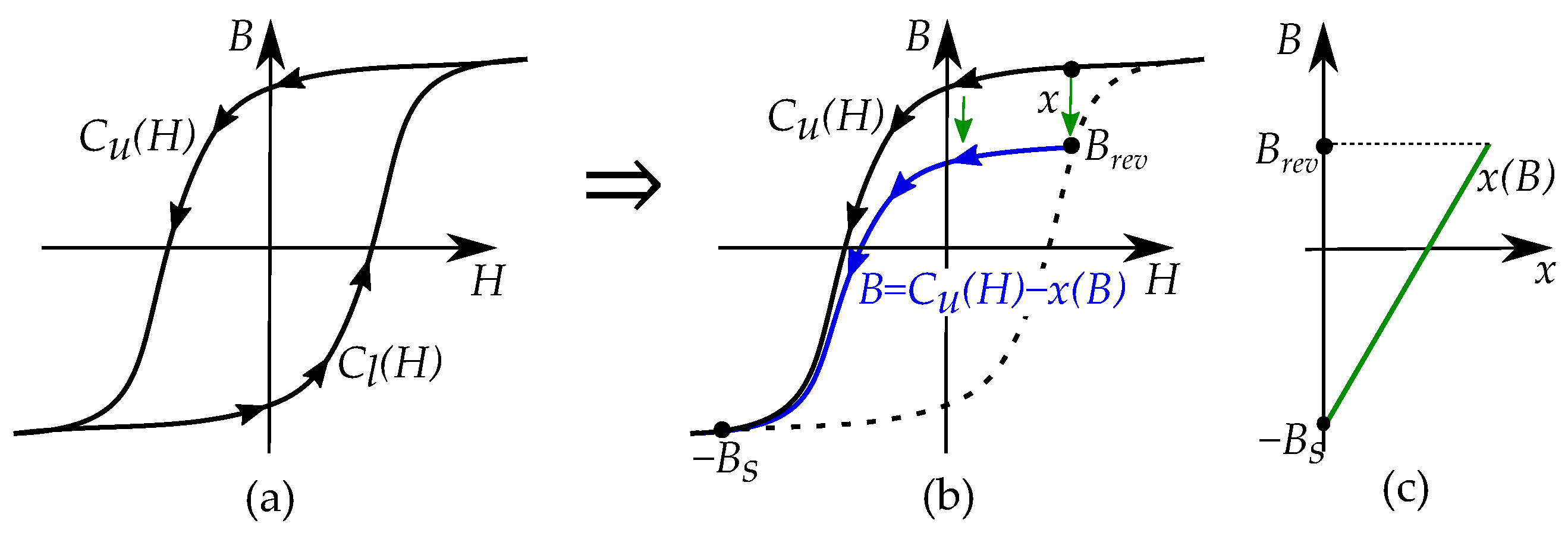
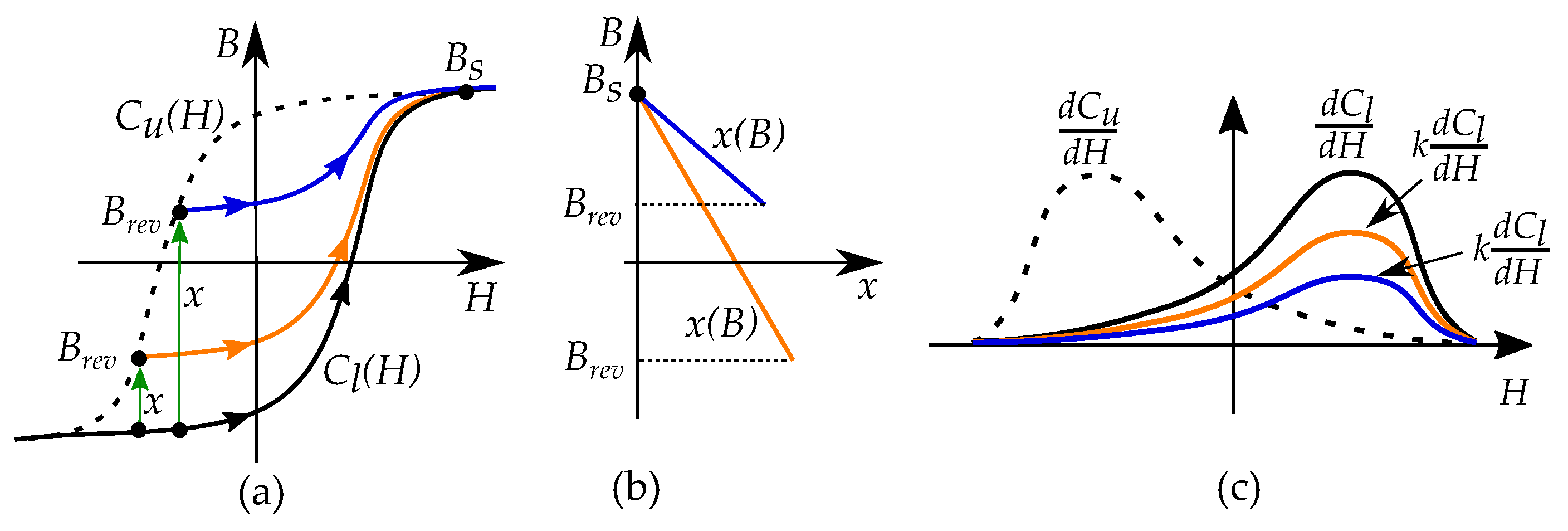
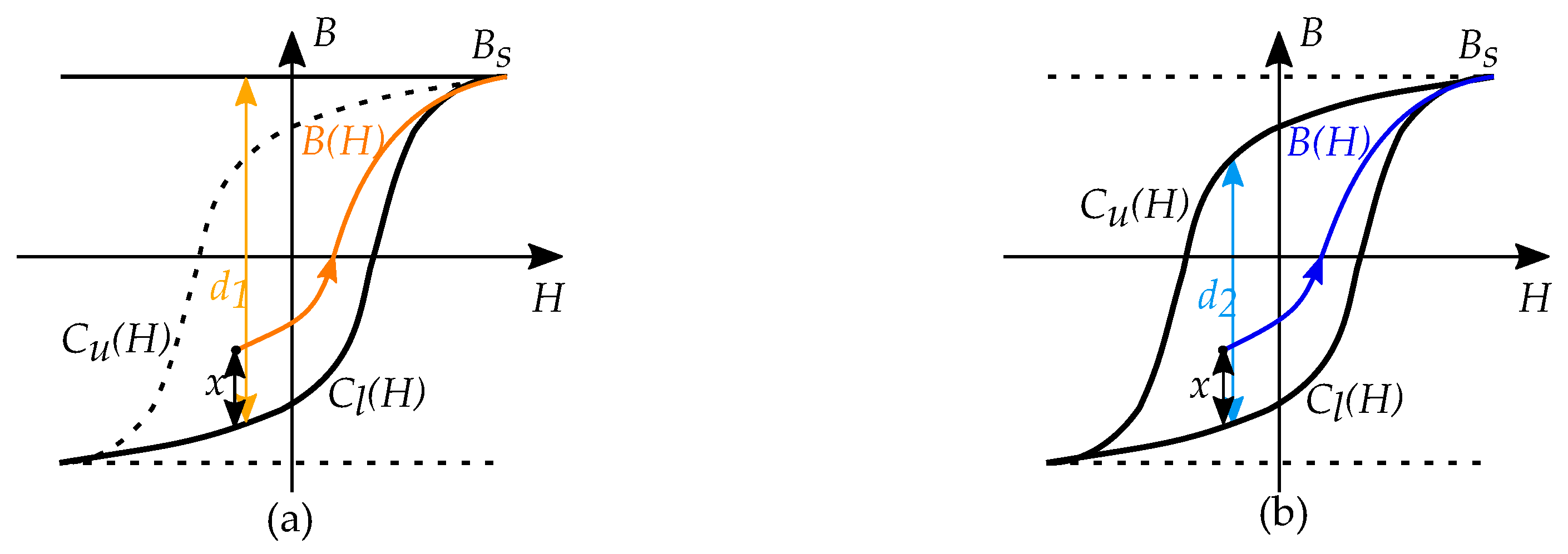
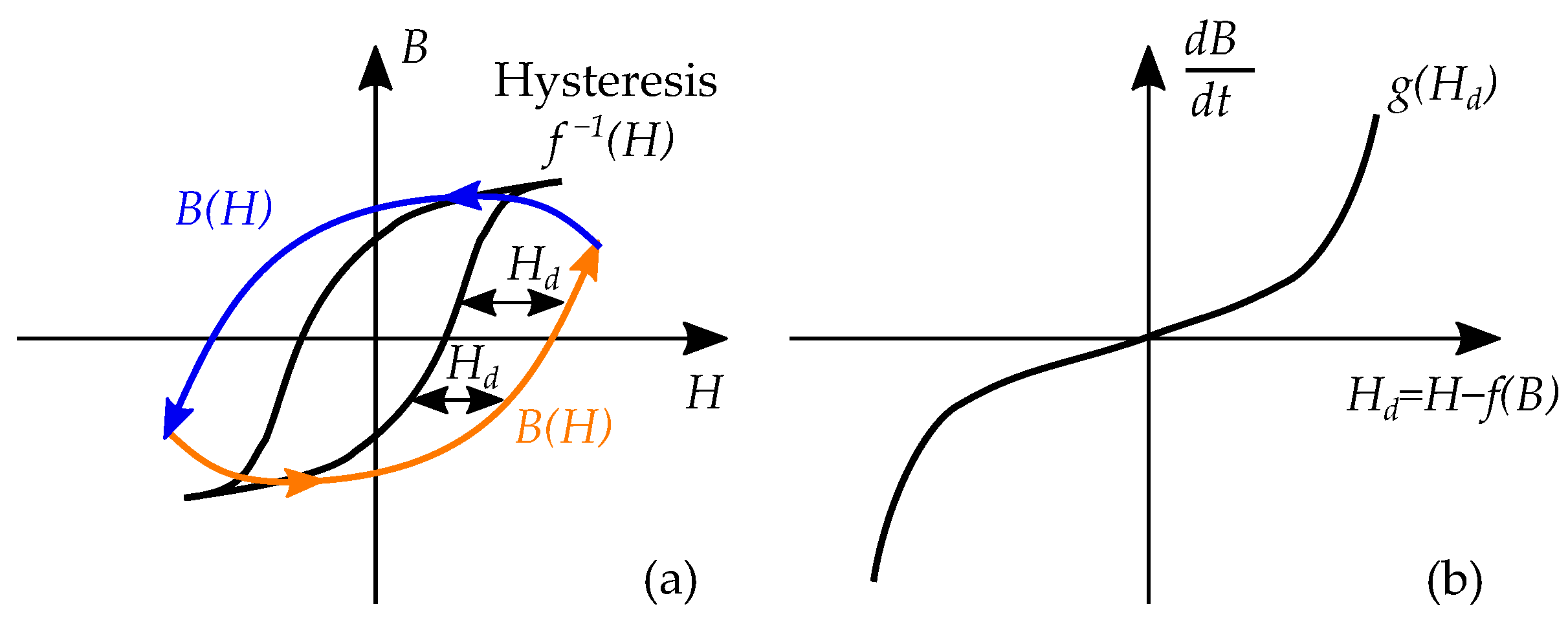
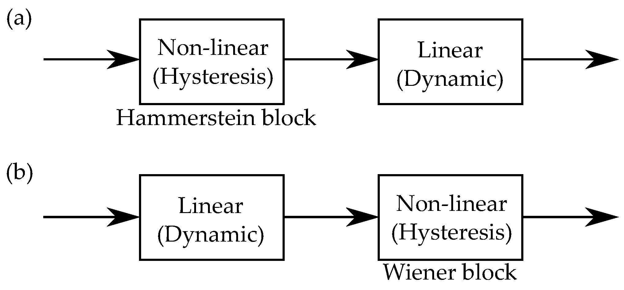
Figure 1. Hysteresis seen in the recoil path for a generic hard magnetic material. At ( B 1 , H 1 ), the magnetic field strength changes direction. The recoil path is different from the previous path, described by the phenomenon called branching.
Energies 16 03908 g001
Figure 2. (a) Generic Duhem model, illustrating the two categories of curves: ascending and descending. (b) A cyclic trajectory is based on the two sets of curves, and will create a hysteresis loop.
Energies 16 03908 g002
Figure 3. (a) Upper limiting boundary. (b) Lower limiting boundary. (c) Major loop curves.
Energies 16 03908 g003
Figure 4. (a) Anhysteresis function. (b) Limits expressed by the distance to the anhysteresis curve.
Energies 16 03908 g004
Figure 5. Example of function f ( H ) and g ( H ) . (a) Simple linear anhysteresis function f ( H ) with saturation levels, and a function g ( H ) ; (b) S-shaped anhysteresis function f ( H ) , and a function g ( H ) .
Energies 16 03908 g005
Figure 6. (a) Illustrating a B ( H ) -curve in the Coleman-Hodgdon model, and its distance x to the anhysteresis curve f ( H ) . (b) The change in distance, d x / d H depends on the distance, x. As the function B ( H ) drifts from f ( H ) , the slope d B / d H will gradually intercept d f / d H . The gradual interception depends on the parameter α and the distance from the anhysteretic function f ( H ) .
Energies 16 03908 g006
Figure 7. Illustrating the basic nomenclature of hysteresis curves.
Energies 16 03908 g007
Figure 8. (a) The major loop, and First order reversal curves (FORCs). (b) Concentric symmetric cycles, with both the major loop and minor loops).
Energies 16 03908 g008
Figure 9. All curves will be based on first order reversal curves and the major loops. (a) A symmetric cycle will be based on trajectories of FORCs. (b) An asymmetric cycle could be based on the major loop curve and a FORC. (c) Drifting occurs when the trajectory of the cycle is not closed.
Energies 16 03908 g009
Figure 10. (a) The curves of the major loop. (b) Generating a set of increasing curves. (c) Generating a set of decreasing curves.
Energies 16 03908 g010
Figure 11. (a) The model generates reversal curves based on downscaled major loop curves. (b) Example showing a hysteresis loop based on the major loop curve and a FORC.
Energies 16 03908 g011
Figure 12. (a) Major loop curve. (b,c) Examples of reversal curves in the model. The curves are downscaled by the factor k, based on k = d K / d .
Energies 16 03908 g012
Figure 13. (a) Major loop curves, expressed on the inverse form H ( B ) . (b) Translated curve, by a constant shift. (c) Translated curve, shifted by a linear function x ( B ) .
Energies 16 03908 g013
Figure 14. (a) Major loop curves. (b) The curve shifted a distance set by the linear function x ( B ) . (c) The linear function x ( B ) decreases towards the saturation point B s .
Energies 16 03908 g014
Figure 15. (a) Example of two reversal curves in the Talukdar–Bailey model. (b) The linear functions x ( B ) used for the two reversal curves. (c) The two curves could instead be generated by downscaling the major loop curve by the factor k.
Energies 16 03908 g015
Figure 16. The method of scaled curves could give undesired trajectories that excides the major loop curves. (a) Example with a reversal curve within the major loop curves. (b) Example of a reversal curve that goes beyond the major loop curve, and leaves the hysteresis area.
Energies 16 03908 g016
Figure 17. Tellinen model is based on decreasing the derivative. (a) One reversal curve based on distances d and x. (b) Decreased derivative by factor k. (c) Set of increasing reversal curves.
Energies 16 03908 g017
Figure 18. Two different types of scaling: (a) The Talukdar–Bailey model, (b) The Tellinen model.
Energies 16 03908 g018
Figure 19. The Flatley–Henretty model rescales the recoil paths based on the major loops. Unlike the Talukdar–Bailey model, the rescaled path is based on the horizontal magnetic field strength distance, w, from the major loop. (a) The distance w is based on the position H and the position H p at the major loop. (b) The curve B ( H ) goes towards the major loop. (c) The curve B ( H ) is based on the major loop, and downscaled based on a function k ( w ) , dependent on the distance w.
Energies 16 03908 g019
Figure 20. An example of Frölich equation. With the example shown as a function of the absolute value | H | , to show the full anhysteresis curve. The curve shape depends on the parameters, here showing a = 1 and b = 0.5 .
Energies 16 03908 g020
Figure 21. (a) The law of approach to saturation describes the curve near magnetic saturation M s . (b) It is useful for modelling curves in high magnetizations, M. (c) There are also adoptions with empirical functions, used for anhysteresis curves (then representing both high and low fields).
Energies 16 03908 g021
Figure 22. (a) Curved shape of Rayleigh model. (b) Hysteresis loop by Rayleigh model. (c) The model is mostly useful for the low flux densities B (i.e. in the Rayleigh region).
Energies 16 03908 g022
Figure 23. (a) Model with exponent n (in H n ). (b) Model with exponent 1 / n (in H 1 / n ).
Energies 16 03908 g023
Figure 24. (a) Model for low fields. (b) Model for high fields. (c) Combined model (describing an initial curve).
Energies 16 03908 g024
Figure 25. Sigmoid functions can be used to approximate the behavior of soft magnetic materials. Illustrating hyperbolic tangent function ( t a n h , blue), inverse tangent function ( a r c t a n , orange) and Langevin function ( L ( x a ) , yellow).
Energies 16 03908 g025
Figure 26. Madelung’s rules for history-dependent hysteresis. The trajectory is defined by the history of reversal points. (a) A first order reversal curve is defined for each point along the major loop. (b) Each curve goes back to the previous-to-last reversal point. (c) When a cycle is closed, the trajectory follows the curve before the cycle.
Energies 16 03908 g026
Figure 27. Numbering of reversal curves based on reversal points.
Energies 16 03908 g027
Figure 28. Examples of Preisach relay hysterons. Each relay only have two states, and the point where it switches between the two state depends on the present state.
Energies 16 03908 g028
Figure 29. (a) Example of a Play operator. Acting like a backlash element. (b) Example of a Stop operator. Acting like a linear function between a maximum and minimum value.
Energies 16 03908 g029
Figure 30. Congruency of loops for cycles within the same interval. The curves will look the same for cycles between H 1 and H 2 , with the same change in B ( same Δ B ).
Energies 16 03908 g030
Figure 31. (a) Example based on a FORC from point P 1 to P 2 . (b) Case of a Duhem model: A SORC would not be properly represented in the model. The curve would act like a FORC and go towards the saturation point B s , instead of towards P 1 . (c) Case with scaling adjusted for return point memory: An improved history dependence would instead have a proper SORC that goes towards the previous-to-last reversal point P 1 .
Energies 16 03908 g031
Figure 32. Comparison between a Hysteron and a Duhem model (or “Prehysteron”). (a) A hysteron model avoids the risk of drifting. (b) A Duhem model results in a risk of drifting curves.
Energies 16 03908 g032
Figure 33. (a) Phasor model of B ( H ) with complex permeability. (b) The hysteresis loop is modelled like an ellipse, without the characteristic branching, but still frequency independent. (c) The hysteresis loop in the model is equivalent to a phase shift δ between B and H.
Energies 16 03908 g033
Figure 34. (a) Illustrating a permeability μ without imaginary part for a linear relation of B ( H ) . (b) Illustrating a relation of B ( H ) from a complex permeability. The complex permeability is different from other hysteresis models since it gives an elliptic loop instead of branching, but the model is still frequency independent. (c) A complex permeability model of eddy currents is instead frequency dependent.
Energies 16 03908 g034
Figure 35. Example illustrating magnetizing loops for frequencies f 1 < f 2 < f 3 < f 4 , at the same interval of H. Higher frequencies result in wider loops, with a more ellipse shaped cycle.
Energies 16 03908 g035
Figure 36. The Chua, or Chua–Stromsmoe model. (a) The loop is expressed by the combination of an dynamic part H d and an anhysteretic function f 1 ( H ) . (b) The dynamic part H d is nonlinear (described by g ( H d ) ), similar to excess eddy current losses.
Energies 16 03908 g036
Figure 37. A frequency-dependent model could be combined with a hysteresis model. (a) The model combines the dynamic part H d with a hysteresis model f 1 ( H ) . (b) The dynamic part could be a non-linear function g ( H d ) .
Energies 16 03908 g037
Figure 38. Examples of speed-dependent hysterons. The width of the loop will increase for higher frequencies. (a) Example of frequency dependent Preisach hysteron (relay). (b) Example of frequency dependent play hysteron.
Energies 16 03908 g038
Figure 39. (a) A Hammerstein model is when the nonlinear part is before the linear part. (b) A Wiener model is the opposite, with a nonlinear part after a linear part.
Energies 16 03908 g039
Table 1. Description of parameters.
ParameterExplanation
M s Saturation magnetization
α Effective field parameter, linked to magnetization
aShape parameter, for anhysteretic curve
cReversibility coefficient
kLinked to hysteresis loss
Disclaimer/Publisher’s Note: The statements, opinions and data contained in all publications are solely those of the individual author(s) and contributor(s) and not of MDPI and/or the editor(s). MDPI and/or the editor(s) disclaim responsibility for any injury to people or property resulting from any ideas, methods, instructions or products referred to in the content.

