Estimating the Performance Loss Rate of Photovoltaic Systems Using Time Series Change Point Analysis

Abstract

The accurate quantification of the performance loss rate of photovoltaic systems is critical for project economics. Following the current research activities in the photovoltaic performance and reliability field, this work presents a comparative assessment between common change point methods for performance loss rate estimation of fielded photovoltaic installations. An extensive testing campaign was thus performed to evaluate time series analysis approaches for performance loss rate evaluation of photovoltaic systems. Historical electrical data from eleven photovoltaic systems installed in Nicosia, Cyprus, and the locations’ meteorological measurements over a period of 8 years were used for this investigation. The application of change point detection algorithms on the constructed monthly photovoltaic performance ratio series revealed that the obtained trend might not always be linear. Specifically, thin film photovoltaic systems showed nonlinear behavior, while nonlinearities were also detected for some crystalline silicon photovoltaic systems. When applying several change point techniques, different numbers and locations of changes were detected, resulting in different performance loss rate values (varying by up to 0.85%/year even for the same number of change points). The results highlighted the importance of the application of nonlinear techniques and the need to extract a robust nonlinear model for detecting significant changes in time series data and estimating accurately the performance loss rate of photovoltaic installations.

1. Introduction

Estimating accurately the performance loss rate (PLR) of fielded photovoltaic (PV) systems is vital for evaluating the lifetime performance output, decreasing financial/investment risks, and improving the bankability [1]. The PLR expresses the performance loss over time with units of %/year and its estimation can be made at different levels (e.g., module, array, inverter and/or system level) based on the available measurements. On the system level, it represents all performance losses such as physical degradation, shade, soiling, snow, etc. [2]. Such losses can be reversible (i.e., loss mechanisms that can be recovered) or irreversible (i.e., loss mechanisms that cannot be retrieved due to physical PV module degradation).

PLR investigations can be performed using indoor or outdoor methodologies. For indoor methods, current–voltage (I–V) curve data and power at standard test conditions (STC) [3] are acquired for PV modules over different time periods. To this end, the PV electrical characteristics are originally measured at STC, and subsequently, the PV panels are exposed either indoors (through accelerated tests) or outdoors [3]. For the PV modules under study, I–V curves are frequently obtained using solar simulators. The differences in the PV electrical parameters from the initial measurements provide evidence of the PLR at successive time periods. The outdoor performance assessment of PV systems can be performed by obtaining I–V sweeps (taken at maximum power point) over different time periods and regular time intervals. Apart from I–V scans, recorded environmental and PV electrical field data (from a data acquisition system) can be used for quantifying long-term performance loss rates. This is achieved through the statistical/comparative analysis of field measurements. This work focuses on PLR investigations using outdoor methodologies and historical field data.

In this domain, the PLR (or the degradation rate when considering only the irreversible material degradation of PV modules) of PV systems is mainly calculated through the statistical extraction of a trend (de-trending) from a performance indicator time series. An influential hypothesis made in past PLR studies was that the subsequent trend was linear. Several statistical techniques have been proposed in the literature for estimating the linear PLR (or the degradation rate) of fielded PV systems [2,4], while also demonstrating that its estimation is methodology-dependent [2]. Reported linear trend extraction methods include the ordinary least squares (OLS) regression, simple- or dual-periodicity fit, the nonparametric filtering method of locally weighted scatterplot smoothing (LOESS), the classical seasonal decomposition (CSD), the Holt–Winters (HW) exponential smoothing, the autoregressive integrated moving average (ARIMA) and the principal component analysis (PCA) [5]. In parallel, a comparative approach (i.e., the year-on-year method) was also introduced in [4,6], and implemented as an open-source Python package [7], for estimating the PLR value. An ensemble method was finally suggested [8] and developed as an open-source R package to calculate the linear PLR [9].

For operating PV systems, a lot of performance outliers reflecting module defects and failures, initial degradation for the case of thin film modules, shading, and soiling can cause performance variations, biasing the PLR results. Special care should be taken for such variations, that can cause nonlinearities in the performance trend of a PV system. Bearing this in mind, the latest studies [1,10,11,12,13] introduced methodological pipelines for estimating the nonlinear PLR (or degradation rate) of PV systems during actual field exposure. In this context, change point (CP) techniques that can identify changes in the investigated performance time series were introduced. More specifically, Facebook Prophet (FBP) was proposed for nonlinear trend extraction in [1], while a multi-step performance loss algorithm using piecewise (or segmented) regression was introduced in [10] for advanced PV system performance loss rate modeling. Segmented regression was also used along with the Bayesian estimation of abrupt change, seasonality, and trend (Beast) in [12] for modeling nonlinear PV degradation rates. The results demonstrated that the segmented method was the most accurate for estimating the degradation rates when using synthetic datasets. Furthermore, the pruned exact linear time (PELT) method was utilized in [13] to estimate the long-term PV degradation rate. The findings of this study showed that the PELT technique could provide more accurate results than conventional statistical models for nonlinear degradation patterns. Moreover, six open-source Python and R libraries were used for a comparative assessment between change point techniques for the nonlinear degradation rate estimation [11]. The results of the analysis demonstrated that piecewise regression (implemented in R and Python) and FBP outperformed the Beast, breakpoint (bkp), and sequential and batch change detection utilizing parametric and nonparametric techniques. The findings of this study also indicated the effectiveness of change point techniques for modeling and decomposing the performance time series and identifying changes in PV performance profiles.

Following the current research activities, the aim of this paper is to advance the field of PV performance and reliability by evaluating common change point techniques for calculating the PLR of fielded PV installations. This paper expands on our previous work [14], where different statistical techniques were evaluated for nonlinear PLR estimation using outdoor field measurements. In this work, the analysis is expanded by presenting the results of an extensive testing evaluation of time series analytic approaches for estimating the PLR and validating the results through indoor testing and synthetically generated PV performance data.

The proposed paper presents useful insights for establishing robust models for capturing both linear and nonlinear PV behavior. Applying methodologies that also consider nonlinear behavior can improve PLR estimates, thus reflecting more accurately PV power plant project economics.

2. Materials and Methods

The procedure followed to estimate the PLR of fielded PV systems using statistical analysis methods is presented in this section. The first section describes the experimental setup (i.e., the investigated PV arrays) and the data acquisition process for extracting and storing the historical outdoor measurements (i.e., PV electrical and meteorological data). Then, it provides details regarding the data processing procedure followed for creating the cleansed PV datasets for analysis. Finally, it describes the methodologies used for PLR estimation and the validation process.

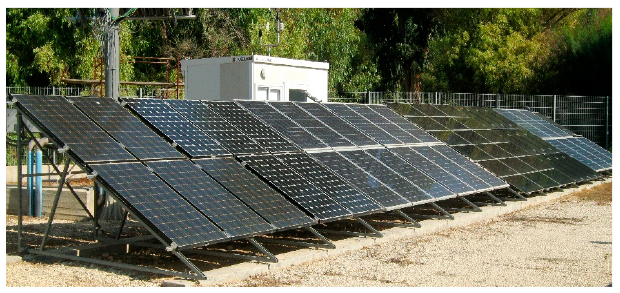
2.1. Experimental Setup and Data Acquisition

Historical data from eleven PV systems were used for this analysis. The test PV systems are of ~1 kW_p capacity and comprise different PV module technologies, including mono-crystalline silicon (mono-c Si), multi-crystalline silicon (multi-c Si), and thin film (i.e., amorphous silicon (a-Si), cadmium telluride (CdTe), copper indium gallium diselenide (CIGS)).

Table 1. Summary of the characteristics of the installed PV systems.

System ID	Manufacturer	Technology	Series Modules	Parallel Module	Rated Power (kWp)
(a)	Atersa	mono-c Si	6	1	1.020
(b)	BP Solar	mono-c Si	6	1	1.110
(c)	Sanyo	mono-c Si	5	1	1.025
(d)	Suntechnics	mono-c Si	5	1	1.000
(e)	Schott Solar	multi-c Si (edge defined film-fed growth—EFG)	6	1	1.000
(f)	Schott Solar	multi-c Si (multi-crystalline advanced industrial cells—MAIN)	4	1	1.020
(g)	SolarWorld	multi-c Si	6	1	0.990
(h)	Solon	multi-c Si	7	1	1.540
(i)	Würth Solar	thin film (CIGS)	6	2	0.900
(j)	First Solar	thin film (CdTe)	3	6	1.080
(k)	Mitsubishi Heavy Industries (MHI)	thin film (a-Si)	2	5	1.000

depicts the characteristics of the installed PV systems.

The PV performance and the weather conditions are recorded every second according to the International Electrotechnical Commission (IEC) 61724-1:2021 standard [15], through the use of a sensor network and a data acquisition system (Campbell Scientific CR1000 with an accuracy of ±0.06%). The recorded measurements are then stored on a monitoring platform as 15 min average measurements. The meteorological measurements include in-plane irradiance (G_I), ambient temperature (T_amb), module temperature (T_mod), wind speed (S_w), and direction (a_w). The electrical data include the array DC current (I_A), voltage (V_A), and power (P_A).

Table 2. Sensor’s network and accuracy.

Parameter	Manufacturer Model	Accuracy
Ambient temperature	Rotronic HC2A-S3	±0.1 °C at 23 °C
In-plane irradiance	Kipp Zonen CMP11	±2% expected daily accuracy, ±20 W/m2 for 1000 W/m2
DC voltage	Muller Ziegler Ugt	±0.5%
DC current	Muller Ziegler Igt	±0.5%
AC energy	Muller Ziegler EZW	±1%

summarizes the installed sensors and the associated measurement accuracies. The PV systems and in-plane irradiance sensors under study were cleaned periodically (i.e., four times a year) and after dust events to decrease the effect of soiling [14]. Systematic recalibration and frequent cross-checks against nearby sensors were performed to identify sensor drifts.

The grid-connected PV systems were commissioned in June 2006 at the outdoor test facility (OTF) of the University of Cyprus (UCY) in Nicosia, Cyprus (Köppen-Geiger-Photovoltaic climate classification CH; steppe climate with high irradiation [16]). The PV arrays, comprising of PV modules connected in series, are installed side-by-side in the south direction and at a constant tilt angle of 27° (see Figure 1).

Historical measurements over a period of 8 years (June 2006–June 2014) were employed for this investigation. The in-plane solar irradiation in Nicosia, Cyprus varied between 1980 kWh/m²/year and 2094 kWh/m²/year. The monthly total in-plane irradiation over the investigated period is provided in Figure 2a. Moreover, the average monthly ambient temperature (19.5 ± 0.5 °C) in Nicosia, Cyprus is shown in Figure 2b.

During the evaluation period, different fault types occurred affecting the PV performance. For example, partial shade affected the performance of the BP Solar and Solon PV systems during the years 2006–2009 [17]. In addition, a fault occurring due to water ingress was reported for the Sanyo and Suntechnics PV systems in March 2009 and June 2009, respectively.

2.2. Data Processing and Creation of PV Datasets

Initially, data quality algorithms were applied to the recorded measurements to cleanse the data [18]. During this procedure, the irradiance measurements were restricted between 0 W/m² and 1300 W/m². Other data filters and statistical tests were also used to filter out invalid values (e.g., outliers, missing and nonrepresentative values) [19].

Next, the PV datasets of each system were created using the filtered measurements and aggregated into monthly blocks. The monthly array performance ratio (PR) was then estimated [20] and incorporated into the PV datasets. For PV arrays, the PR is defined as (1):

PR = Y_f/Y_r

(1)

where Y_f is the final yield and Y_r is the reference yield.

Subsequently, an outlier filter (i.e., three-sigma) was employed to remove outlying values [21]. Figure 3 illustrates the PR time series for the PV systems under investigation. All PV technologies exhibit seasonal behavior (i.e., higher performance values in winter months and lower values in the summer period mainly due to module temperature variations), with the thin film technologies exhibiting a slowly progressing performance loss.

The exhibited monthly PR time series of the investigated PV arrays are depicted in Figure 4. The crystalline silicon PV systems exhibited similar behavior and PR variations (i.e., same seasonal performance pattern) over the years, apart from the BP Solar system (whose modules were partially shaded). The BP Solar PV system achieved the lowest PR variations among the crystalline silicon PV systems. In addition, the crystalline silicon PV systems demonstrated greater peak-to-peak PR variations than the thin film PV arrays. Signs of early degradation are evident for the thin film technologies. Findings from previous studies [22,23] demonstrated pronounced performance loss during the first months of operation for the First Solar and MHI thin film systems due to the stabilization processes.

2.3. PLR Estimation Using Statistical Methods

Different statistical techniques, such as the LOESS method and change point algorithms, were utilized to calculate the linear/nonlinear PLR of the investigated PV arrays. The LOESS method utilizes local weighted regression fitting [24] and a smoother is used to decompose the given time series into three components (trend, seasonal, remainder). The OLS method is then applied to the LOESS trend to estimate the linear PLR. The LOESS estimates are not affected by outliers and they can be utilized to estimate nonlinearities [24]. In this paper, the LOESS trend was also inspected visually to detect change points in the performance time series.

Change point algorithms were then used for identifying changes in PV trends and estimating the linear (in case of zero change points) or nonlinear (in case of 1 or more change points) PLR. More specifically, the PELT, the bkp, the FBP, and the Beast algorithms were utilized.

The PELT method was utilized to identify change points in the performance ratio time series [25] for a specified cost function and penalty [26]. To avoid overfitting (e.g., identifying noise as change points), penalty values were used as inputs. In this work, the optimal segmentations for multiple penalty values over a continuous range were selected (i.e., from 0.001 to log10(x)—where x is the total number of months in the performance time series). Once the change points were detected, a small t-test was performed to extract the significant change points [27]. The procedure followed for identifying the significant change points is as follows [28]:

(1)

Each change point corresponds to two data segments (e.g., one segment from the start month of the reporting period to the corresponding month of the change point, and the other from the change point month to the end month of the time series) with supposedly different means. In case of more than one change point, the number of segments is equal to the number of change points plus one (number of segments = number of change points + 1).

(2)

For each change point, we subtract the data of its second segment from the data of its first segment (i.e., the data difference, x_d) and ensure that the months of the subtracted data correspond. If the detected change point is not statistically significant, then the mean of x_d should be statistically zero. Otherwise, if the mean of x_d is not statistically zero, then the detected change point is statistically significant.

(3)

We test the following hypothesis (assuming that the differences x_d,i are random from normal distribution such as the E (x_d,i) = 0):

• Null hypothesis H₀: E (x_d,i) = 0
• Alternative hypothesis H_α: Ε(x_d,i) $\ne$ 0

If the null hypothesis (H₀) is rejected, the data provide evidence in favor of the alternative hypothesis (H_α).

The bkp algorithm uses linear regression models for detecting changes within the time series [29], by minimizing the residual sum of squares [30]. In this work, the bkp algorithm was utilized to identify multiple change points in time series regression models using Bellman’s principle of optimality [30]. To determine the ideal number of breaks, the Bayesian information criterion estimator of the number of change points was utilized.

The Beast algorithm deals with Bayesian CP detection and time series decomposition. It uses a Bayesian model averaging scheme to decompose the time series into abrupt changes (i.e., CPs), cyclic variations (e.g., seasonality) and trends (i.e., piecewise linear and nonlinear) [31]. The period for the seasonal/cyclic component (which was set to 12 for the annual time series) and the max number of trend change points (which was set to 3) allowed in segmenting and fitting the trend component were provided as inputs (specified by the user). More details about the Beast algorithm and the calibration process are provided in [32].

The FBP algorithm is an additive model, in which nonlinear trends are fit with yearly, weekly, and daily seasonality, plus holiday effects. The FBP model decomposes the time series into trend, seasonality, and holidays [33]. A piecewise linear model is employed to model the trend component, while an additive component is used for modeling seasonality. A number of CPs are distributed uniformly along the time series. Then, it statistically compares the slopes to a predefined threshold level to determine the significant CPs. The tuning of the FBP algorithm was executed as reported in [1].

Once the CPs were detected by the four algorithms, the trend was sliced into different segments (with the number of segments being equal to the number of detected change points + 1), and finally, the OLS method was applied to calculate the PLR of each segment.

2.4. Validation through Indoor Testing and Synthetic Dataset

The obtained time series analysis results were thus validated through indoor testing. In particular, the test PV systems were tested indoors at STC to measure the electrical characteristics of each PV module according to the IEC 61215-1 [34]. These characteristics were then used to estimate the linear PLR at STC. The indoor measurement procedure took place inside a solar simulator (i.e., the Pasan SunSim IIIc). The technical procedure followed for indoor testing along with the calibration process are described in detail by Phinikarides et al. in [3]. In parallel, electroluminescence (EL) and infrared (IR) thermography images were also taken for each test PV module to detect any invisible defects, which can cause performance drops.

Finally, the PR time series of the Sanyo system was used to create a PV performance time series (see Figure 5) with anomalous conditions (circled in red). This system was selected as it is a well-maintained and well-operating PV system, showing PR values between 0.80 and 0.97 and availability of higher than 99% during the reporting period [19]. The time series was generated to investigate the effectiveness of CP models for estimating the PLR in the presence of data anomalies (here only global and local outliers were emulated), that may be attributed to fault occurrences and/or maintenance events.

3. Results and Discussion

The obtained PLR results for the fielded PV arrays along with the findings from the application of outdoor time series analysis techniques and indoor STC are presented in this section. Future research directions are also provided.

3.1. Linear PLR Estimates Using the LOESS Technique

The LOESS method was applied to the constructed monthly performance time series to obtain the respective PV trend (see Figure 6). The LOESS trend was also inspected visually for detecting change points within the given time series. Initial inspection of the trend indicated obvious trend changes (and the presence of nonlinear power loss) for the BP Solar and thin film PV arrays. Since there were indications for the existence of change point(s), the utilization of change point algorithms is needed for more reliable PLR estimations.

This method was then used to estimate the linear PLR (see

Table 3. Annual PLR of the PV arrays under study evaluated by the LOESS method.

System ID	Annual PLR (%/Year) ± Standard Error
(a)	−0.78 ± 0.00
(b)	−0.60 ± 0.01
(c)	−0.74 ± 0.00
(d)	−0.75 ± 0.00
(e)	−0.84 ± 0.00
(f)	−0.68 ± 0.00
(g)	−1.09 ± 0.00
(h)	−1.09 ± 0.00
(i)	−2.52 ± 0.03
(j)	−2.04 ± 0.00
(k)	−1.46 ± 0.00

). The annual PLR values ranged from −0.60 to −2.04%/year, which is in line with the reported literature values [2]. For the mono-c Si PV arrays, the PLR estimates varied between −0.60 and −0.78%/year. Likewise, the obtained PLR values for the multi-c Si PV systems ranged from −0.68 to −1.09%/year. As indicated by the results, all crystalline silicon-based PV arrays demonstrated annual PLR < 1%/year.

Conversely, the thin film technologies yielded greater annual PLR values (when compared to crystalline silicon-based technologies), varying from −1.46 to −2.52%/year. Similar results (PLR values larger than −1%/year and ranging between −0.6 and −2.4%/year) were reported in the literature for thin film PV systems [10].

The histogram of the PLR, the median and mean for all investigated PV systems using the LOESS technique is shown in Figure 7. The median PLR for all PV module technologies was −0.84%/year and is shown by the red dashed vertical line. The mean PLR of all technologies was −1.14%/year (black dashed vertical line). For individual technologies, the mean PLR for mono-crystalline silicon was −0.72%/year, for multi-crystalline silicon was −0.93%/year, and for thin film the mean was −2.01%/year. The differences in the mean PLR indicate that a separation must be made, according to the PV module technology.

3.2. Nonlinear PLR Estimates Using CP Algorithms

Four different change point methods were subsequently employed to find PV trend changes and calculate the nonlinear power loss. Specifically, the PELT technique revealed at least one change point for all the PV systems under study as indicated in

Table 4. Change points identified by the PELT algorithm.

System ID	Number of CPs	Location of CPs
(a)	2	04/2011, 10/2013
(b)	3	03/2008, 12/2009, 04/2012
(c)	1	04/2008
(d)	1	04/2008
(e)	1	02/2011
(f)	2	05/2012, 09/2012
(g)	1	03/2009
(h)	1	02/2009
(i)	2	04/2008, 03/2012
(j)	2	04/2008, 04/2011
(k)	2	11/2008, 12/2011

. Two change points were detected for the Atersa, Schott Solar (EFG), Würth Solar, First Solar, and MHI arrays. The detected change point in 2008 for the thin film PV technologies may be attributed to initial degradation. Finally, three change points were identified for the BP Solar system in 2008 (probably due to partial shading), 2009 (probably due to partial shading), and 2012. Likewise, partial shading may be the cause for the change point detected in 2009 for the Solon PV system. For the rest of the PV systems, information extracted from the maintenance logs did not indicate any fault/maintenance event. Therefore, some of the identified change points might be due to the actual degradation mode.

For demonstration reasons, the changes detected by the PELT technique for two test PV systems (i.e., the BP Solar and MHI), for which suspicions were created by the visual inspection of the LOESS trend, are shown in Figure 8.

The bkp algorithm also identified at least one CP for all PV installations as shown in

Table 5. Change points identified by the bkp algorithm.

System ID	Number of CPs	Location of CPs
(a)	1	04/2011
(b)	2	03/2008, 08/2009
(c)	1	04/2008
(d)	1	04/2008
(e)	1	02/2011
(f)	1	03/2012
(g)	1	03/2009
(h)	1	02/2009
(i)	3	04/2008, 04/2010, 04/2012
(j)	3	03/2008, 02/2010, 01/2012
(k)	3	10/2007, 12/2008, 12/2011

. Two change points were identified for the BP Solar PV system in 2008 and 2009 (years when the system was affected by partial shading conditions), while three change points were found for all the thin film PV systems. For the MHI PV system, the detected change points in 2007 and 2008 may be due to initial degradation.

The Beast algorithm also detected CPs for nine PV systems (see

Table 6. Change points identified by the Beast algorithm.

System ID	Number of CPs	Location of CPs
(a)	2	09/2011, 10/2013
(b)	2	09/2008, 03/2010
(c)	1	09/2010
(d)	1	08/2009
(e)	0	-
(f)	2	01/2009, 02/2012
(g)	0	-
(h)	2	02/2009, 02/2012
(i)	1	07/2012
(j)	1	06/2012
(k)	3	09/2008, 11/2009, 12/2011

), while zero CPs were identified for the Schott Solar MAIN and SolarWorld PV arrays. One CP was detected for the Sanyo, Suntechnics, Würth Solar, and First Solar systems. For the Suntechnics PV system, the identified CP may be due to a failure reported in the log. Three changes in the PR time series were detected for the MHI PV system; two of them may be attributed to early degradation. For the Atersa and Schott Solar (EFG) PV systems, two CPs were detected, with no indications of fault occurrences in the logs. Likewise, two CPs were identified for the BP Solar and Solon PV systems, with their maintenance logs reporting some performance issues.

Zero CPs were identified for Atersa, Schott Solar (MAIN and EFG), and SolarWorld PV systems when applying the FBP algorithm (see

Table 7. Change points identified by the FBP algorithm.

System ID	Number of CPs	Location of CPs
(a)	0	-
(b)	2	12/2008, 05/2011
(c)	1	07/2009
(d)	1	04/2009
(e)	0	-
(f)	0	-
(g)	0	-
(h)	1	05/2011
(i)	1	06/2011
(j)	1	08/2009
(k)	1	04/2010

). One change point was identified for Sanyo and Suntechnics PV arrays in 2009 (might be caused by water ingress reported failure in 2009) as well as for the Solon PV system (affected by partial shading). One change point was also identified for the thin film PV arrays in the early years of operation. Finally, two CPs in 2008 and 2011 were identified for the BP Solar system.

The detected change points for each PV system and per algorithm are depicted in Figure 9. Different numbers of change points were identified depending on the utilized technique. The results demonstrate that the PLR estimation is methodology dependent. For the thin film technologies, all algorithms identified at least one change point, indicating that the PV trend can demonstrate nonlinearities that need to be accounted for (particularly for this PV module technology).

In addition, even different locations of change points were identified for the same PV system using different methods (see Figure 10). Consequently, different PLR values will be obtained by each method. This highlights the necessity of deriving more sophisticated and accurate models for PLR estimations of fielded PV systems.

Then, the nonlinear PLR was estimated. Here, only the results from the FBP application are displayed, since this method has already been benchmarked using synthetic data and the results provided evidence for robust PLR estimates [1,11,12]. The FBP results are summarized in

Table 8. Annual PLR of PV systems under study obtained from the application of FBP algorithm.

System ID	Linear FPB	FPB PLR1	FPB PLR2	FPB PLR3
(a)	−0.83 ± 0.01	-	-	-
(b)	-	−4.27 ± 0.01	−2.49 ± 0.01	−1.42 ± 0.01
(c)	-	−1.35 ± 0.01	−0.45 ± 0.01	-
(d)	-	−1.07 ± 0.00	−0.61 ± 0.00	-
(e)	−0.96 ± 0.00	-	-	-
(f)	−0.80 ± 0.00	-	-	-
(g)	−1.23 ± 0.00	-	-	-
(h)	-	−1.21 ± 0.01	−0.90 ± 0.01	-
(i)	-	−2.52 ± 0.00	−2.66 ± 0.01	-
(j)	-	−2.80 ± 0.00	−1.99 ± 0.04	-
(k)	-	−1.78 ± 0.01	−1.48 ± 0.00	-

. For the case of linear trend (i.e., Atersa mono-c Si, Schott Solar multi-c Si (MAIN), Schott Solar multi-c Si (EFG) and SolarWorld multi-c Si PV systems), differences of up to 0.14% were observed when compared to LOESS linear PLR estimates.

The other three CPs were also used for calculating the PLR of PV systems. The acquired values of PLR showed differences up to 0.85%/year (for the same number of change points) between the CP methods.

3.3. Indoor Testing Results and Validation

The indoor testing results showed variations in the maximum power point of PV modules within the array after outdoor field exposure. From the obtained EL images (see Figure 11), broken cells and cracks were detected for two of the test PV arrays (BP Solar and SolarWorld), justifying their low performance and the detection of change points within their time series.

The FBP method, which demonstrated nonlinear PLR estimation and fault categorization capabilities in PV systems [35,36], was then validated against the created Sanyo PV performance time series with data anomalies. The results are shown in Figure 12, verifying the FBP model’s capability for capturing trend changes, even in the presence of global/local outliers in the time series. It can be seen, that the FBP model detected the same CP (July 2009) as previously (see Section 3.2) for the Sanyo PV system. FBP is thus a robust model for reliability studies and the initial results showed that its performance is not affected by outliers. Though further validation is needed to confirm the model’s accuracy in the presence of anomalous conditions, that will be part of future investigations.

3.4. Summary and Future Directions

The performed investigation showed valuable information for the PLR of fielded PV systems and the following findings were obtained:

• The LOESS trend can be used for an initial screening to detect obvious change points within the PV performance time series.
• The application of change point algorithms proved to be an efficient statistical technique for detecting nonlinear power loss in PV systems.
• The identified change points may be attributed to failures/defects, maintenance events and/or actual degradation mechanisms. Suggestions for future research include the development of a detailed methodology for attributing the reason (e.g., maintenance events, fault, and degradation modes) behind the detected change points.
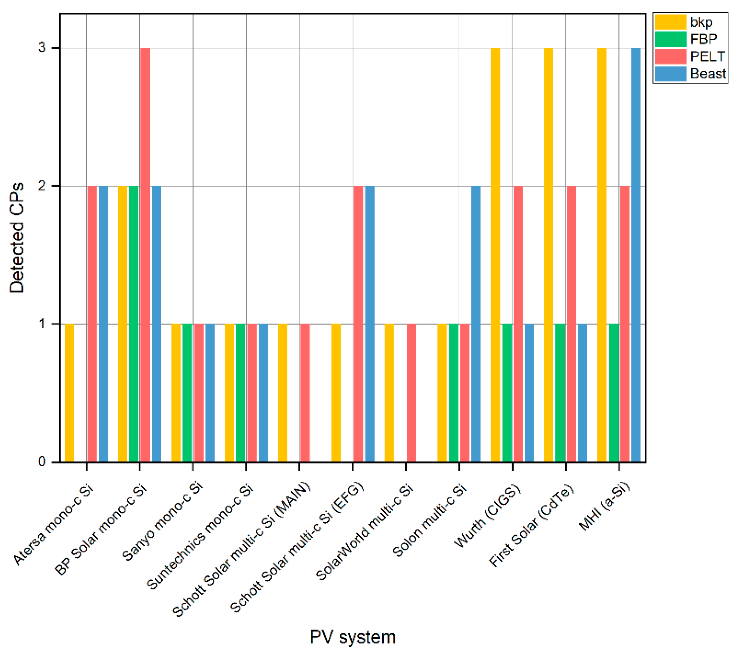
• Different numbers and locations of change points were detected based on the applied algorithm. This reveals the method dependency of the PLR estimation.
• The indoor testing validation revealed invisible defects that may be the root cause of PV’s low performance and the existence of change points.
• The validation of the FBP model on the created PV performance time series with data anomalies showed its capability for capturing trend changes, even in the presence of anomalous conditions. Though, further investigation and validation on data with different types of outliers, such as global (i.e., point anomalies), contextual (i.e., conditional anomalies), and collective outliers, is needed to verify the above statement.

Apart from the validation of the FBP model against outlying conditions, future work should focus on the application of the LOESS method for quantifying nonlinear behavior and estimating the PLR. Moreover, due to the immersion of new PV module technologies (e.g., advanced crystalline silicon cells accounting for ~25% of market share), further investigation is needed for such novel technologies, which would be the focus of future research.

4. Conclusions

In this work, the annual performance loss rate of various technology PV systems was estimated by utilizing statistical analysis methods, applied on outdoor field measurements. The analysis revealed that the extracted trend might exhibit nonlinearities. To identify nonlinear performance loss in PV systems, the application of change point algorithms proved to be an effective solution. The change point algorithms can identify changes in PV trends. Though, different numbers and locations of change points were identified based on the applied methodology. As a result, different performance loss rate values were obtained by each change point algorithm, demonstrating differences up to 0.85% per year (for the same number of change points). This illustrates the methodology dependency of the performance loss rate estimates. By cross-correlating the identified change point location with the maintenance logs, the results revealed that the change points may be due to failures, maintenance events and/or actual degradation mechanisms. Though, further research is required to determine the reason behind the detected change points.

Since the performance loss rate directly influences the LCOE, the need for more sophisticated models is thus required for estimating accurately this rate for operating PV systems. Future research should thus focus on the extraction of the PV performance trend by the LOESS method to quantify nonlinear behavior and precisely estimate the performance loss rate values. The performance loss rate estimation’s sensitivity to outliers is also recommended. Finally, estimating the performance loss rate of novel solar PV technologies should be the focus of future research.

References

1. Theristis, M.; Livera, A.; Jones, C.B.; Makrides, G.; Georghiou, G.E.; Stein, J.S. Nonlinear Photovoltaic Degradation Rates: Modeling and Comparison Against Conventional Methods. IEEE J. Photovolt. 2020, 10, 1112–1118. [Google Scholar] [CrossRef]
2. Phinikarides, A.; Kindyni, N.; Makrides, G.; Georghiou, G.E. Review of Photovoltaic Degradation Rate Methodologies. Renew. Sustain. Energy Rev. 2014, 40, 143–152. [Google Scholar] [CrossRef]
3. Phinikarides, A.; Makrides, G.; Georghiou, G.E. Estimation of Annual Performance Loss Rates of Grid-Connected Photovoltaic Systems Using Time Series Analysis and Validation through Indoor Testing at Standard Test Conditions. In Proceedings of the 2015 IEEE 42nd Photovoltaic Specialist Conference, New Orleans, LA, USA, 14–19 June 2015; pp. 1–5. [Google Scholar] [CrossRef]
4. Jordan, D.C.; Deceglie, M.G.; Kurtz, S.R. PV Degradation Methodology Comparison—A Basis for a Standard. In Proceedings of the 2016 IEEE 43rd Photovoltaic Specialists Conference (PVSC), Portland, OR, USA, 5–10 June 2016; pp. 273–278. [Google Scholar] [CrossRef]
5. Livera, A.; Phinikarides, A.; Makrides, G.; Georghiou, G.E. Impact of Missing Data on the Estimation of Photovoltaic System Degradation Rate. In Proceedings of the 2017 IEEE 44th Photovoltaic Specialist Conference (PVSC), Washington, DC, USA, 25–30 June 2017; pp. 1954–1958. [Google Scholar] [CrossRef]
6. Jordan, D.C.; Deline, C.; Kurtz, S.R.; Kimball, G.M.; Anderson, M. Robust PV Degradation Methodology and Application. IEEE J. Photovolt. 2018, 8, 525–531. [Google Scholar] [CrossRef]
7. Deceglie, M.G.; Jordan, D.; Shinn, A.; Deline, C. RdTools: An Open Source Python Library for PV Degradation Analysis Degradation Rate; National Renewable Energy Lab. (NREL): Golden, CO, USA, 2018; pp. 1–15.
8. Curran, A.J.; Jones, C.B.; Lindig, S.; Stein, J.; Moser, D.; French, R.H. Performance Loss Rate Consistency and Uncertainty Across Multiple Methods and Filtering Criteria. In Proceedings of the 46th IEEE Photovoltaic Specialist Conference (PVSC), Chicago, IL, USA, 16–21 June 2019; pp. 1328–1334. [Google Scholar]
9. Curran, A.; Burleyson, T.; Oltjen, W.; Lindig, S.; Moser, D.; French, R.; Solar Durability and Lifetime Extension Research Center. PVplr: SDLE Performance Loss Rate Analysis Pipeline. Available online: https://cran.r-project.org/package=PVplr (accessed on 21 April 2023).
10. Lindig, S.; Louwen, A.; Moser, D.; Topic, M. New PV Performance Loss Methodology Applying a Self-Regulated Multistep Algorithm. IEEE J. Photovolt. 2021, 11, 1087–1096. [Google Scholar] [CrossRef]
11. Theristis, M.; Livera, A.; Micheli, L.; Ascencio-Vásquez, J.; Makrides, G.; Georghiou, G.E.; Stein, J.S. Comparative Analysis of Change-Point Techniques for Nonlinear Photovoltaic Performance Degradation Rate Estimations. IEEE J. Photovolt. 2021, 11, 1511–1518. [Google Scholar] [CrossRef]
12. Theristis, M.; Livera, A.; Micheli, L.; Jones, B.; Makrides, G.; Georghiou, G.E.; Stein, J. Modeling Nonlinear Photovoltaic Degradation Rates. In Proceedings of the 47th IEEE Photovoltaic Specialist Conference (PVSC), Calgary, AB, Canada, 15 June–21 August 2020; pp. 0208–0212. [Google Scholar]
13. Romero-Fiances, I.; Livera, A.; Theristis, M.; Makrides, G.; Stein, J.S.; Nofuentes, G.; de la Casa, J.; Georghiou, G.E. Impact of Duration and Missing Data on the Long-Term Photovoltaic Degradation Rate Estimation. Renew. Energy 2022, 181, 738–748. [Google Scholar] [CrossRef]
14. Livera, A.; Tziolis, G.; Theristis, M.; Stein, J.S.; Georghiou, G.E. Performance Loss Rate Estimation of Fielded Photovoltaic Systems Based on Statistical Change- Point Techniques. In Proceedings of the 2022 2nd International Conference on Energy Transition in the Mediterranean Area (SyNERGY MED), Thessaloniki, Greece, 17–19 October 2022; pp. 1–6. [Google Scholar]
15. IEC 61724-1:2021; Photovoltaic System Performance—Part 1: Monitoring. IEC: Geneva, Switzerland, 2021.
16. Ascencio-Vásquez, J.; Brecl, K.; Topič, M. Methodology of Köppen-Geiger-Photovoltaic Climate Classification and Implications to Worldwide Mapping of PV System Performance. Sol. Energy 2019, 191, 672–685. [Google Scholar] [CrossRef]
17. Makrides, G.; Zinsser, B.; Schubert, M.; Georghiou, G.E. Energy Yield Prediction Errors and Uncertainties of Different Photovoltaic Models. Prog. Photovolt. Res. Appl. 2013, 21, 500–516. [Google Scholar] [CrossRef]
18. Livera, A.; Theristis, M.; Koumpli, E.; Theocharides, S.; Makrides, G.; Sutterlueti, J.; Stein, J.S.; Georghiou, G.E. Data Processing and Quality Verification for Improved Photovoltaic Performance and Reliability Analytics. Prog. Photovolt. Res. Appl. 2021, 29, 143–158. [Google Scholar] [CrossRef]
19. Livera, A.; Theristis, M.; Koumpli, E.; Makrides, G.; Stein, J.S.; Georghiou, G.E. Guidelines for Ensuring Data Quality for Photovoltaic System Performance Assessment and Monitoring. In Proceedings of the 37th European Photovoltaic Solar Energy Conference (EU PVSEC), Online, 7–11 September 2020; pp. 1352–1356. [Google Scholar]
20. Theristis, M.; Venizelou, V.; Makrides, G.; Georghiou, G.E. Chapter II-1-B—Energy Yield in Photovoltaic Systems. In McEvoy’s Handbook of Photovoltaics, 3rd ed.; Kalogirou, S.A., Ed.; Academic Press: Cambridge, MA, USA, 2018; pp. 671–713. ISBN 9780128099216. [Google Scholar]
21. Livera, A.; Florides, M.; Theristis, M.; Makrides, G.; Georghiou, G.E. Failure Diagnosis of Short- and Open-Circuit Fault Conditions in PV Systems. In Proceedings of the 45th IEEE Photovoltaic Specialist Conference (PVSC), Waikoloa, HI, USA, 10–15 June 2018; pp. 0739–0744. [Google Scholar]
22. Makrides, G.; Zinsser, B.; Schubert, M.; Georghiou, G.E. Performance Loss Rate of Twelve Photovoltaic Technologies under Field Conditions Using Statistical Techniques. Sol. Energy 2014, 103, 28–42. [Google Scholar] [CrossRef]
23. Phinikarides, A.; Makrides, G.; Zinsser, B.; Schubert, M.; Georghiou, G.E. Analysis of Photovoltaic System Performance Time Series: Seasonality and Performance Loss. Renew. Energy 2015, 77, 51–63. [Google Scholar] [CrossRef]
24. Cleveland, R.; Cleveland, W.; McRae, J.; Terpenning, I. STL: A Seasonal-Trend Decomposition Procedure Based on Loess. J. Off. Stat. 1990, 6, 3–73. [Google Scholar]
25. Killick, R.; Fearnhead, P.; Eckley, I.A. Optimal Detection of Changepoints with a Linear Computational Cost. J. Am. Stat. Assoc. 2012, 107, 1590–1598. [Google Scholar] [CrossRef]
26. Jackson, B.; Scargle, J.D.; Barnes, D.; Arabhi, S.; Alt, A.; Gioumousis, P.; Gwin, E.; Sangtrakulcharoen, P.; Tan, L.; Tsai, T.T. An Algorithm for Optimal Partitioning of Data on an Interval. IEEE Signal Process. Lett. 2005, 12, 105–108. [Google Scholar] [CrossRef]
27. Academy, S. Introductory Statistics; v. 1.; Saylor Academy: Washington, DC, USA, 2012. [Google Scholar]
28. Livera, A. Analytical Monitoring System for the Reliable Diagnosis of Failures in Grid-Connected Photovoltaic Systems. Ph.D. Thesis, University of Cyprus, Nicosia, Cyprus, 2022. [Google Scholar]
29. Bai, J.; Perron, P. Estimating and Testing Linear Models with Multiple Structural Changes. Econometrica 1998, 66, 47–48. [Google Scholar] [CrossRef]
30. Bai, J.; Perron, P. Computation and Analysis of Multiple Structural Change Models. J. Appl. Econom. 2003, 18, 1–22. [Google Scholar] [CrossRef]
31. Zhao, K.; Wulder, M.A.; Hu, T.; Bright, R.; Wu, Q.; Qin, H.; Li, Y.; Toman, E.; Mallick, B.; Zhang, X.; et al. Detecting Change-Point, Trend, and Seasonality in Satellite Time Series Data to Track Abrupt Changes and Nonlinear Dynamics: A Bayesian Ensemble Algorithm. Remote Sens. Environ. 2019, 232, 111181. [Google Scholar] [CrossRef]
32. Micheli, L.; Theristis, M.; Livera, A.; Stein, J.S.; Georghiou, G.E.; Muller, M.; Almonacid, F.; Fernández, E.F. Improved PV Soiling Extraction through the Detection of Cleanings and Change Points. IEEE J. Photovolt. 2021, 11, 519–526. [Google Scholar] [CrossRef]
33. Taylor, S.J.; Letham, B. Forecasting at Scale. Am. Stat. 2017, 72, 37–45. [Google Scholar] [CrossRef]
34. IEC 61215-1:2016; Terrestrial Photovoltaic (PV) Modules—Design Qualification and Type Approval—Part 1: Test Requiremnts. International Electrotechnical Commission: Geneva, Switzerland, 2016.
35. Livera, A.; Theristis, M.; Makrides, G.; Georghiou, G.E. Intelligent Cloud-Based Monitoring and Control Digital Twin for Photovoltaic Power Plants. In Proceedings of the 49th IEEE Photovoltaic Specialist Conference (PVSC), Philadelphia, PA, USA, 5–10 June 2022; pp. 0267–0274. [Google Scholar]
36. Livera, A.; Theristis, M.; Micheli, L.; Stein, J.S.; Georghiou, G.E. Failure Diagnosis and Trend-Based Performance Losses Routines for the Detection and Classification of Incidents in Large-Scale Photovoltaic Systems. Prog. Photovolt. Res. Appl. 2022, 30, 921–937. [Google Scholar] [CrossRef]
Figure 1. PV arrays installed at the UCY in Nicosia, Cyprus.
Energies 16 03724 g001
Figure 2. (a) Total in-plane irradiation aggregated into monthly values and (b) average ambient temperature in Nicosia, Cyprus over the evaluation period.
Energies 16 03724 g002
Figure 3. Monthly PR time series for the PV systems under investigation from June 2006–June 2014.
Energies 16 03724 g003
Figure 4. Monthly PR time series for (a) mono-crystalline silicon (mono-c Si), (b) multi-crystalline silicon (multi-c Si), and (c) thin film PV systems over the evaluation period (June 2006–June 2014).
Energies 16 03724 g004
Figure 5. PR time series of the Sanyo PV system with emulated data anomalies (circled in red).
Energies 16 03724 g005
Figure 6. Monthly PR time series along with the LOESS trend (colored in maroon) for the investigated PV systems. The purple, black, and red lines indicate the mono-crystalline silicon (mono-c Si), multi-crystalline silicon (multi-c Si), and thin film PV systems, respectively.
Energies 16 03724 g006
Figure 7. Histogram of PLR of all PV systems using the LOESS technique. The red and black vertical lines indicate the median and the mean PLR, respectively.
Energies 16 03724 g007
Figure 8. Monthly PR time series for the (a) BP Solar (mono-c Si) and (b) MHI thin film (a-Si) PV arrays. The solid maroon line indicates the LOESS trend, while the red dashed vertical lines show the position of the detected CPs.
Energies 16 03724 g008
Figure 9. Detected change points for the investigated PV systems using different techniques.
Energies 16 03724 g009
Figure 10. Location of detected CPs for all PV systems under study using different techniques.
Energies 16 03724 g010
Figure 11. Obtained EL images from defective PV modules. Detected defects include cracked cells and hotspots.
Energies 16 03724 g011
Figure 12. PR time series (shown by black dots) of the Sanyo PV system with imputed data anomalies. The change point detected by FBP algorithm is shown in red dashed line. The red and blue solid lines show the extracted trend and FBP fit, respectively. The blue-shaded area is the uncertainty.
Energies 16 03724 g012