Article

Experimental and Numerical Analysis of the Effect of Rheological Models on Measurements of Shear-Thinning Fluid Flow in Smooth Pipes

by
Abdalsalam Ihmoudah
1,2,*,
Abdelsalam Abugharara
1,3,
Mohammad Azizur Rahman
4 and
Stephen Butt
1
1
Faculty of Engineering & Applied Science, Memorial University of Newfoundland, St. Johns, NL A1C 5S7, Canada
2
College of Engineering, Wadi Alshatti University, Alshatti P.O. Box 68, Libya
3
Faculty of Energy and Mining, Sebha University, Sebha P.O. Box 18758, Libya
4
Petroleum Engineering, Texas A&M University at Qatar, Doha 23874, Qatar
*
Author to whom correspondence should be addressed.
Energies 2023, 16(8), 3478; https://doi.org/10.3390/en16083478
Submission received: 18 March 2023 / Revised: 9 April 2023 / Accepted: 14 April 2023 / Published: 16 April 2023
(This article belongs to the Section H1: Petroleum Engineering)

Abstract

:
The aim of this research is to investigate the effects of rheological models of shear-thinning fluids and their estimated parameters on the predictions of laminar, transitional, and turbulent flow. The investigation was carried out through experimental and computational fluid dynamics (CFD) studies in horizontal pipes (diameters of 19.1 mm and 76.2 mm). Six turbulent models using Reynolds averaged Navier–Stokes equations in CFD_ANSYS Fluent 19.0 were examined in a 3D simulation followed by comparison studies between numerical and experimental results. Regarding results of laminar regions in power-law rheology models, Metzner and Reed presented the best fit for the pressure loss and transitional velocity. For the turbulent region, correlations observed by Wilson and Thomas as well as Dodge and Matzner had good agreement with the experimental results. For Herschel–Bulkley fluids, pressure losses and transitional regions based on a yielded region were examined and compared to the experimental results and the modified Slatter Reynolds number, where the results provided good estimation. For both pipe diameters, the Slatter model was the best fit for pressure losses of Herschel–Bulkley fluids in the turbulent regime. Furthermore, when comparing k-omega and k-epsilon turbulence models to the power-law behaviour, numerical studies delivered the most accurate results with fluids that have a higher behaviour index. However, the error percentage significantly increased at a higher shear rate in the Herschel–Bulkley fluids with a greater yield stress effect. Moreover, the modified Herschel–Bulkley viscosity function by Papanastasiou was implemented in the current CFD study. This function was numerically stabilized, devoid of discontinuity at a low strain rate, and more effective in transitional regions.

1. Introduction

Non-Newtonian fluids flowing in pipelines can be found in a wide range of practical and industrial applications. Non-Newtonian flow behaviour in the laminar region, which is related to rheological properties and pressure losses, could be predicted by integrating the constitutive rheological model. On the other hand, the prediction of pressure losses in turbulent flow remains one of the most theoretical and practical problems [1,2]. Most of the fluids used at drilling sites are categorized as having non-Newtonian behaviour with non-linear viscosity, which makes it difficult to predict turbulent pressure losses in pipes. The mismatch between the rheological models and the properties of drilling fluids can lead to serious issues during drilling operations, such as loss of well control, reduced carrying capacity, fluid losses, and stuck pipes [3]. Rheological parameters of non-Newtonian fluids can assist in providing a description of fluid models. Those relevant parameters include yield stress, consistency index, fluid behaviour index, and density as a volumetric parameter [4]. Such parameters are important for predicting frictional pressure loss; however, all these parameters could change in conditions of high and low pressure and temperature, which could have a direct effect on drilling fluid rheology via the fluid’s shear stress and shear rate [5,6,7,8,9]. In designing pipelines and drilling mud circulation for non-Newtonian fluids, pressure drops and transient limitations are among the most important technical parameters that could influence pumping energy requirements. Pressure drops could occur due to internal fluid friction as well as friction between the fluid and the pipe wall. Literature shows that there is a lack of recent studies that report the effect of rheological properties of shear-thinning fluid, especially Herschel–Bulkley fluid, in real flow conditions on flow measurements in pipes. The power-law model has been widely applied to obtain relationships between flow rate and pressure drop at a low Reynolds number in various geometries, including expanding and elastic pipes [10,11]. Several recent studies investigated various hydrodynamic problems involving shear-thinning fluids at low Reynolds numbers and clearly demonstrated a limited range of applicability for power-law model [12,13].
The aim of this study is to experimentally and numerically investigate the effect of the choice of the rheological model on predicting pipe flow characteristics for a laminar, transitional, and turbulent flow. This study also evaluates the ability of computational fluid dynamics (CFD) in the turbulent model of ANSYS Fluent 19 to simulate non-Newtonian fluids with various rheological behaviours. The experimental data of this work were obtained for two shear-thinning rheological models (power-law and Herschel–Bulkley fluids) that were prepared and used in this study. Moreover, the performance of three tested materials, including carboxymethyl cellulose (CMC), bentonite, and Xanthan gum, were fitted to the laminar flow data and evaluated based on the nonlinear fits’ root-mean square error (RMSE) [14,15].

2. Background and Theory

2.1. Rheological Models

There is no direct proportionality between shear stress and shear rate in non-Newtonian fluids. Therefore, in order to describe the rheological behaviour of non-Newtonian shear-thinning fluids, different flow models are used. Equations (1) and (2) present the power-law and the Herschel–Bulkley models used in this study [2,16].

2.2. The Power-Law Model

For a power-law fluid, a relationship between shear stress and shear rate is described in the form of the following:
τ = k γ ˙ n
where τ is the shear stress,  k  is the fluid’s consistency coefficient, γ˙ is the shear rate, and n is the flow behaviour index. If n > 1, the fluid exhibits shear-thickening properties, and if n < 1, the fluid shows shear-thinning behaviour.

2.3. Herschel–Bulkley Model

The Herschel–Bulkley model combines Bingham and power-law fluid properties. When n < 1, the Herschel–Bulkley model is considered as a shear-thinning fluid model [2,17,18,19]
τ = τ y + k γ ˙ n ( τ > τ o )
where τ is the shear stress,  k  is the fluid consistency coefficient, γ˙ is the shear rate, τy is the yield stress, and n is the flow behaviour index.

2.4. Laminar and Transitional Flow Models

The Rabinowitsch–Mooney relationship is derived for shear stress at the pipe’s wall ( τ w) in relation to the liquid volumetric flow rate (Q/s). The volumetric flow rate and the shear stress are expressed in Equation (3) [2].
Q = π R 3 τ w 3 0 τ w τ r z 2 f τ r z d τ r z
Shear-thinning fluids can be formulated by integrating and substituting the rheological parameters in Equation (3) and then written in terms of 8V/D against τw as in Equations (4) and (5).
Power-law fluid:
8 V D = 4 τ w K 1 n n 3 n + 1
Herschel–Bulkley:
8 V D = 4 τ w 3 τ w τ y ( n + 1 ) / n 1 K 1 n n τ w 2 n + 1 2 n 2 τ y τ w τ y n + 1 2 n + 1 2 n 2 τ w τ y 2 ( n + 1 ) ( 3 n + 1 )
For non-Newtonian transition criteria analysis, the present work uses the approach of Metzner and Reed [20] as the power-law fluid method and Slatter [21] as the Herschel–Bulkley fluid approach. Details on these techniques are provided in the following sections.
Metzner and Reed [20] adapted the Reynolds number to correlate the non-Newtonian pipe flow for a time-independent power-law fluid. In their formulation, the Fanning friction factor was employed as a stability parameter. They proposed that non-Newtonian fluids occur at the limit of the laminar flow as the same Reynolds number of the Newtonian fluids in smooth pipes, which is RMR = 2100 at  f N  = 0.0076 [2], as in Equations (6) and (7).
τ w = K 8 V D n
R M R = 8 ρ v 2 K 8 V D n
The friction factor for the laminar flow was then determined by Metzner and Reed in the same approach as for the Newtonian fluids.
f = 16 R M R

2.5. Current Study Test Model

For the correlation of the laminar flow data, the generalized Reynolds number was developed in this study from the Reynolds number proposed by Slatter [21] by considering the effect of the pipe diameter and the effect of the apparent viscosity. In Herschel–Bulkley fluids, the velocity distribution is discrete into yielded and unyielded regions [2]. As illustrated in Figure 1, in the middle of the pipe (0 ≤ D/2 ≤ Dp/2), an unsheared plug-like core was flowing, where the magnitude of the shear stress was less than that of the yield stress. Dp/2 is the radius of the plug region and depends upon the wall shear stress and the yield stress as follows:
D P / 2 = D / 2 τ y τ w
where Dp/2 is the radius of the plug region, D is the pipe diameter,  τ y  is the yield stress, and  τ w  is the wall shear stress obtained from the laminar flow using Equation (5).
In this study, the modified Reynolds number is based on the fluid density ( ρ ) , the superficial velocity ( v ), the effect of the pipe diameter  D e f f , and the effect of apparent viscosity ( μ e f f ) as in Equation (10) [2]
R e M = ρ v D e f f μ e f f
where  D e f f  is the effect diameter of the pipe as expressed below:
D e f f = D D p
The effect of apparent viscosity is presented in Equation (12)
μ e f f = τ y 8 V D e f f 1 + K 8 V D e f f n 1
where  τ y  is yield stress,  D e f f  is the effect diameter (which can be calculated form Equation (11)),  K  is the consistency coefficient, and n is the flow index.
The fact that when the shear stress is less than the yield stress, as in the unsheared core region, the material will behave as a solid is implicit in the definition of yield stress. Under laminar flow conditions, most models ignore the presence of the unsheared solid plug concentric alignment with the pipe axis due to the presence of yield stress [21]. The pressure drop values measured on the measuring section during flow are sufficient to determine the fluid’s rheological properties, K [22].
Slatter [21] proposed a modified Reynolds number (ReST) that represented yield power-law-type fluid flow, with an emphasis on yield stress. In this formulation, the modified Reynolds number assumes that viscous and inertial forces can be calculated only by the material section undergoing shearing. Laminar flow was taken at ReST = 2100.
R e S T = 8 ρ v a n n 2 τ y + K 8 v a n n D s h e a r n
v a n n = Q Q p l u g π ( R 2 R 2 p l u g )
Q p l u g = V p l u g π D 2 p l u g
V p l u g = n R n + 1 τ y k 1 n ( 1 ) ( n + 1 ) n
where
= D p l u g D τ 0 τ y
D p l u g = 2 R P u l g
D s h e a r = D D p l u g = 2 ( R 2 R 2 p l u g )
In later work on Herschel–Bulkley fluid transition, Slatter [23] demonstrated the ReST as being highly reliable compared to other Reynolds numbers in predicting transitional velocity for different pipe sizes. In particular, for small pipe diameters (D < 25 mm), Slatter [23] reported that every method agreed with the experimental data except the intersection approach reported by Hedström [24]. Vlasak and Chara [25] tested the prediction accuracy of the Slatter [21] model for kaolin slurry turbulent flow and had good results. The researchers discovered that the findings were very similar to those discovered by Wilson and Thomas [26].

2.6. Turbulent Flow Models

A number of different models have been developed for predicting the pressure gradient of shear-thinning turbulent pipe flow. The accuracy, applicability, and limitation of these correlations have been examined. Such correlations considered in this work were proposed by Dodge and Metzner [27], Torrance [28], Yoo [29], Wilson and Thomas [26], and Slatter [21].
Dodge and Metzner [27] devised a critical Reynolds number for their method by applying the friction factor of power-law fluids to a generalized Reynolds number. In so doing, they found that the values of the critical Reynolds number that were determined by their method were in agreement with those determined by Metzner and Reed [20].
1 f = 4.0 n 0.75 l o g R M R f ( 1 n 2 ) 0.4 n 1.2
However, because the experimental results presented that the critical Reynolds number falls in the range of 2900 ≤ RMR ≤ 36,000 and the flow behaviour index is in the range of 0.36 ≤ n ≤ 1, these limits should not be exceeded when applying Equation (20) [30]. Moreover, based on experimental results of shear-thinning fluid, Equation (20) could also be applied to Herschel–Bulkley fluids, Casson fluids, and Bingham plastic if K0 and n0 are determined from the curve of the laminar τw vs. 8V/D at the turbulent flow for the value of τw [3,20].
Torrance [28] investigated the turbulent flow of Herschel–Bulkley fluid based on the pseudoplastic model reported by Clapp [31]. In his work, Torrance assumed that the transitional flow occurs at Re = 2100. When ignoring the effect of the yield stress, Torrance derived the mean velocity for turbulent flow in smooth pipes as follows:
R T o r r = 8 ρ v 2 K 8 V D n = R M R
V U * = 3.8 n + 2.78 n ln 1 τ 0 τ w + 2.78 n + ln U * 2 n ρ R n K 4.17
U * = τ w / ρ
On the other hand, El-Nahhas et al. [1] concluded that the Slatter [21] model that predicts the turbulent flow of Herschel–Bulkley fluid is better than the Torrance model [28], which ignores the impact of the yield stress.
Yoo’s [29] experimental results for power-law fluid presented that the critical Reynolds number falls in the limits of 5000 ≤ RMR ≤ 30,000. These limits should not be exceeded when using Equation (24) [30].
f = 0.079 n 0.675 R M R 0.25 )
Wilson and Thomas [26], followed by Thomas and Wilson [32], proposed a turbulent flow model to predict non-Newtonian flow based on the velocity distribution using enhanced microscale viscosity effects. The model predicts that the wall’s laminar sub-layer increases if the viscous sub-layer size increases by the area ratio factor (α*), as indicated in Equation (25)
V U * = V N U * + 11.6 α * 1 2.5 ln α *
where  U *  is the shear velocity given by Equation (23), and VN is the Newtonian mean velocity for smooth pipe flow as provided below:
V N = U * 2.5 ln ρ D μ e + 1.75
= 2.5 l n ( 1 τ 0 τ w ) + 2.5 τ 0 τ w ( 1 0.5 τ 0 τ w )
For Herschel–Bulkley fluid,  α *  is expressed as follows:
α * = 2 ( 1 + τ 0 τ w n ) / ( 1 + n )
whereas for power-law fluid,  α *  is expressed as follows:
α * = 2 ( 1 1 + n )
Generally, the ratio (α*) represents a combination of expected Newtonian rheogram and non-Newtonian areas occurring near a wall’s shear stress. For each different rheological model (power-law and Herschel–Bulkley fluid), the (α*) first needs to be estimated in order to formulate the velocity distribution of a turbulent model.
Slatter [21] developed an approach for the turbulent flow of Herschel–Bulkley fluid. In his approach, Slatter emphasizes the effect of yield stress based on the effect of particle roughness combined with the Newtonian approach. He formulated a new roughness Reynolds (Rr) by considering the roughness caused by solid particles in smooth wall turbulent flow and fully developed rough-turbulent flow based on percentile passing of particle size (d85) as expressed below:
If Rr < 3.32, then smooth wall turbulent flow exists, and the mean velocity is given by:
V = U * 2.5 ln R / d 85 + 2.5 ln R r + 1.75
where
R r = 8 ρ v * 2 τ y + K 8 v * / d 85 n
If Rr > 3.32, then fully developed rough wall turbulent flow exists, and the mean velocity is given by:
V = U * 2.5 ln R / d 85 + 4.75
In other experiments, Slatter et al. [33] used Equation (31) in Bingham plastic, Hershel–Bulkley fluids, and power-law fluids. These researchers found that the correlation was most applicable to Herschel–Bulkley rheology with an average error of only 18%. In contrast, the power-law model gave an average error of 35%, which was similar to that which resulted from the models of Torrance [28] and Wilson and Thomas [26]. The Bingham plastic fluid model gave errors of about 20%. To date, the Dodge and Metzner [27] correlations are widely applied and quoted in relation to non-Newtonian fluid (power-law fluid) technology (e.g., Skelland [34]; Steffe [35]; Van den Heever [36]; and Chabra and Richardson [2]).

3. Computational Fluid Dynamics (CFD) and Shear-Thinning Fluids

As computational resources are further developed, the analysis of certain industrial flows is increasingly being made by numerical computations using equations of Reynolds averaged Navier–Stokes (RANS). RANS models for shear-thinning fluids, on the other hand, have yet to gain traction in the CFD community as a result of the effect of non-linear viscosity [37,38,39]. The experimental facilities required to conduct these studies could be costly, whereas CFD allows for a wide range of configurations and superficial velocities. Researchers have recently proposed using a combination of turbulence models (i.e., zero, one, and two equations) for predicting homogenous flow. For instance, Stainsby and Chilton [40] developed a hybrid model suitable for application implementing Herschel–Bulkley fluids. In order to explain their observations, the authors combined a modified rheological model with the Launder–Sharma k-ε turbulence model, comparing predictions using high yield stress fluid measurement.
Several numerical studies on non-Newtonian fluid flows in pipelines have been conducted since the development of CFD to compare experimental results and theoretical modelling [41,42]. Most of those studies were related to power-law fluids. In related work to find the apparent viscosity, Bartosik [43] and Bartosik et al. [44] combined a modified turbulence damping function in Launder and Sharma’s k-ε turbulence model [45] with Wilson and Thomas’s hypotheses, thus adapting them to the Bingham rheological model. In so doing, the researchers used the measurements to compare pressure drop predictions for different rheological parameters. The results showed good agreement between the measurements and predictions. Other studies investigated whether the experimental data matched the predicted velocity distribution, with the results confirming satisfactory prediction accuracy [46]. Cayeux and Leulseged [47] developed a general solution for modelling the viscous pressure loss in a pipe under a thixotropic rheological model, and they applied this generic solution to configurations where the diameters change. It was observed that the choice of rheological behaviour should be guided by the actual fluid response, especially in the turbulent flow regime. Recently, methods for estimating fluid rheological properties based on pressure loss measurements were developed by Magnon and Cayeux [48].

4. Experimental Work

Experimental data for this study were collected using two flow loops of diameters 19.1 and 76.2 mm in a laboratory at Memorial University of Newfoundland (MUN), Canada. The setup in which the experiments were carried out is depicted schematically in Figure 2. The large pipe flow loop (Figure 2a) was a clear PVC open-loop re-circulating pipe with a diameter of 0.0762 m and a total length of 65 m. The flow loop included a 3000 L (792.5 gallons) fluid reservoir and a variable-frequency controlled pump with a maximum flow rate of 450 gallons per minute (GPM). An Omega turbine flow meter with an accuracy of ±1% of the full scale and a range of 3~450 GPM was used to measure the flow rate of working fluids. Three PX603-100G5V (0–100 Psi) Omega pressure transducers provided the pressure data in the test sections, and pressure taps positioned 2.5 m from each other were utilized. In the small pipe flow loop (Figure 2b), the working fluids were pumped from the tank through a PVC pipe with a diameter of 0.0191 m and a length of 22 m. Six pressure transducers (Omega PX603-100Q5V, with effective measures of 0–100 psi) were used to measure pressure losses in the test sections at different flow rates.

4.1. Characterization of Test Fluids

To achieve the stated goals, six polymer-based fluids were prepared in the Drilling Technology Laboratory (DTL) at MUN and tested in this study. However, one case that was experimentally adopted by Slatter [21] was considered in this study with a higher yield shear effect for Herschel–Bulkley fluid and compared to the CFD-ANSYS study.
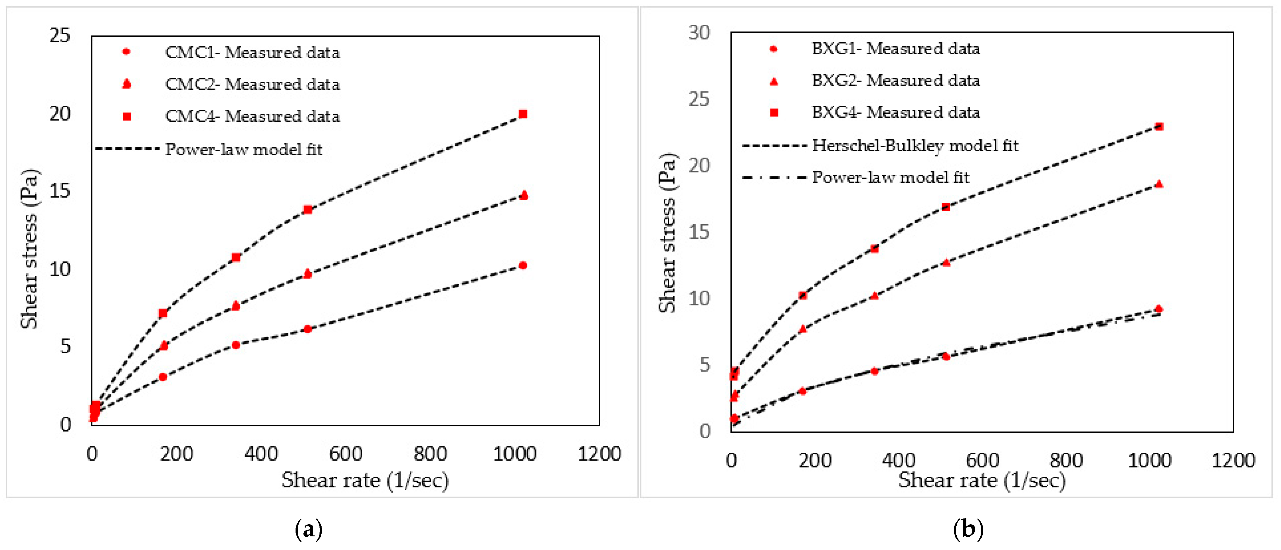
The base fluid for each of these fluids was water. The non-Newtonian fluids tested were shear-thinning fluids (power-law and Herschel–Bulkley fluids). The rheological measurements of the fluids were determined by using an 8-speed API-compliant rotational viscometer (Model 800) and mud balance scale three times during the experiment at the same circulation temperatures. The relationships between shear rates varied between 5.11 and 1022.04 s–1, and shear stress was between 0 and 23 Pa, as shown in Figure 3. The parameters of the shear-thinning rheological fluids (n, K and τy) were obtained by fitting a curve to the rheology (shear stress vs. shear rate graph) from the rotational viscometer data. We used an accurate method to determine the parameters of power-law fluid and three parameters of the Herschel–Bulkley fluid from 8-speed viscometer data following to procedure of Klotz and Brigham [14] and Kelessidis and Maglione [15]. The rheological parameters for each drilling fluid are listed in Section 4.8. When comparing different drilling fluids, the Herschel–Bulkley model with dimensionless shear rates is preferable to the traditional way of writing this model [49].

4.2. Numerical Procedure

In this work, six turbulence models for Newtonian and non-Newtonian fluids in two pipe diameters of 19.1 mm and 76.2 mm were evaluated by comparing the wall shear stress τw obtained from CFD ANSYS Fluent 19.0 with our experimental results. Compute Canada ACENET supercomputers were used for all simulations to solve CFD ANSYS Fluent code. For single-phase models, the turbulence models of Reynolds averaged Navier–Stokes (RANS) can be expressed as follows [50].

4.3. Turbulence Modelling

The present study considered a turbulent regime since experimental critical velocity and modified Reynolds numbers for power-law and Herschel–Bulkley fluids are in the range of turbulent flow. Many models have been developed in CFD codes ANSYS Fluent 19 commercials, such as k-ε models, large eddy simulation (LES), and k-ω models. In this study k-ε  and  k-ω approaches were used, and the classification of Reynolds averaged Navier–Stokes (RANS) was selected to solve two transport equation models are shown below [50]:
k-ε Models
t ρ k + x i ρ k u i = x i µ e f f α k k x j + G k + G b ρ ε
t ρ ε + x i ρ ϵ u i = x i µ e f f α k ε k x j + G ε + G b + ɛ k c 1 ɛ G k + 3 ɛ c b ρ ɛ c 2 ϵ ρ
where k and ε represent turbulence kinetic energy,  G b   a n d   G k  are turbulent kinetic energy generated from buoyancy and mean velocity gradient, c1ε, c2ε, and c3ε are constants, and µeff is the effective viscosity.
k- ω Models,
The k and ω transport equation can be written as:
t ρ k + x i ρ k u i = x i Γ k + k x j + G k Y k + S K
t ρ ω + x i ρ ω u i = x i Γ ω ω x j + G ɛ Y ω + S ɛ
where
Γ k = µ t + µ t ρ k , Γ ω = µ t + µ t ρ ω
where ω is the specific dissipation rate, Γk and Γω are the effective diffusivity of k and ω, Sω is the source term, and Yω is the dissipation of ω.

4.4. Modified Herschel–Bulkley–Papanastasiou Viscosity Model

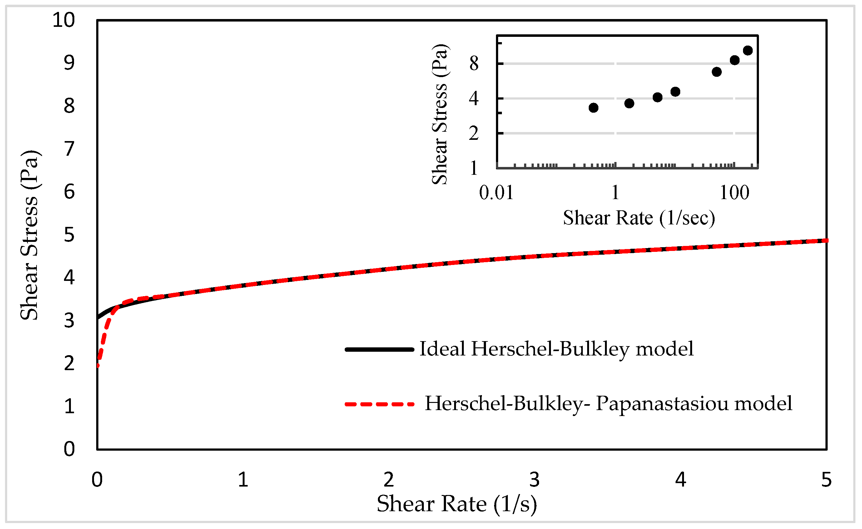
There is a singularity issue associated with the classical Herschel–Bulkley viscosity model at an evanescence shear rate, especially in translucent regions. To alleviate this, Papanastasiou [51] suggested using an exponential regularization for Equation (2) by involving a parameter that not only modulates exponential stress growth but also includes time dimensions. Figure 4 depicts the relationship of shear stress and shear rate using Papanastasiou’s proposed model as well as the effect of the added exponent for Herschel–Bulkley BXG4 fluid. Papanastasiou’s model was later adopted as the Herschel–Bulkley–Papanastasiou model.
τ = K γ ˙ n + τ y 1 e x p ( δ γ ˙ )
The Papanastasiou-modified Herschel–Bulkley viscosity function is not available in general-purpose codes of ANSYS Fluent 19. A new viscosity function was implemented in the current CFD study. This modified viscosity function is numerically stabilized and devoid of discontinuity at a vanishing shear rate.

4.5. Solver and Numerics

CFD ANSYS Fluent [34], which employs a finite-volume method, was used to solve the RANS Equations (33) and (35). A second-order upwind scheme was used to ensure numerical stability during spatial discretization. The SIMPLE scheme was used for pressure–velocity coupling, and the QUICK scheme was used to discretize momentum equations. These schemes were chosen because of their ability to solve momentum and mass conservation equations with reasonable stability and convergence. The RANS models, k-ε and k-ω, were used with the standard model constants, which can be further explored in the ANSYS Fluent 19 guide [50].

4.6. Mesh Size and Grid Study

Mesh size and quality play an important role in CFD studies. Due to the simple geometry of the pipe, a structured hexagonal mesh was used in this simulation. A mesh independence study was performed for all geometric conditions to determine the best number of mesh sizes that gives an acceptable result within a given accuracy and minimum computer operating requirements.
As shown in Figure 5, a 3D computational grid for simulating fluid flow in two different diameters of horizontal pipes were generated and meshed using ICEM meshing techniques. The inlet for both pipes had a specified velocity and turbulence intensity, while the outlet had an outflow condition with mass flow balance. The walls of the pipes were modelled using the specified spear approach. The cells in the pipe wall increase in height towards the centre. This pattern is commonly used with wall functions when simulating turbulent boundary layers [45,49]. Each grid follows the same pattern from the wall to half of the radius, after which the cells were more uniformly arranged into an O-grid. In order to avoid being within the fully laminar or turbulent regimes for the Newtonian standard wall function in the k-ε model, y+ must be within the range of 30 to 300 [52]. To ascertain the grid convergence for non-Newtonian fluids, the height of the first grid point y+ was stabilized at 1.2 in the k-ω model as a correspondence to the increase in the Reynolds number. In the k-ε model with scalable wall functions, the first grid height was y+ ≥ 11.3 and placed gradually further from the wall as the Reynolds number value increased.
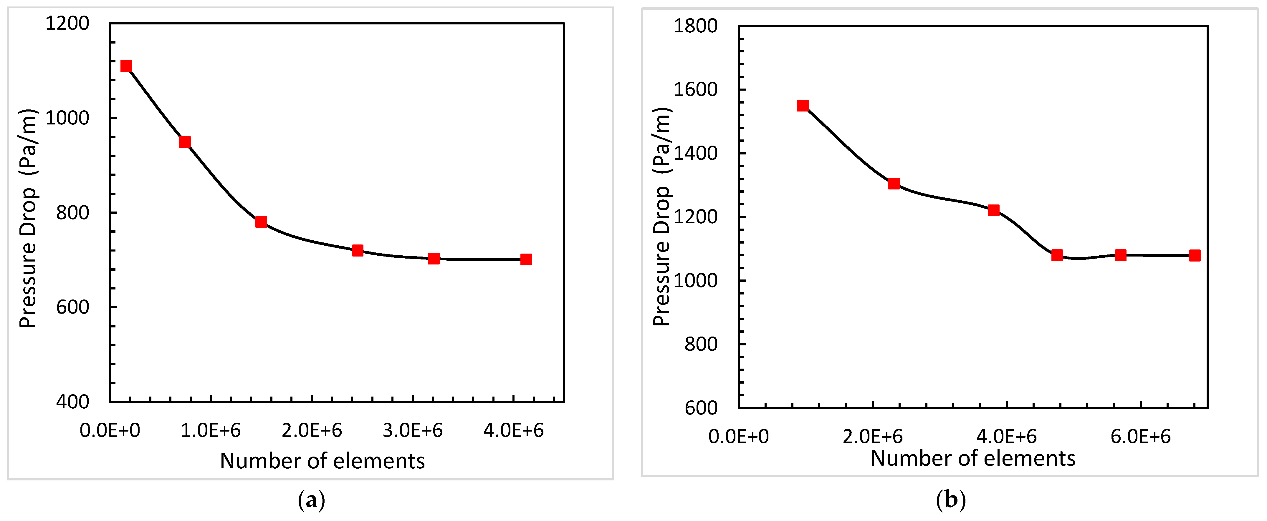
The grid independence analysis for Newtonian and non-Newtonian geometric conditions are shown in Figure 6. Water and shear-thinning fluid (BXG4) with a velocity of 2.205 m/s was used to check the grid study for the horizontal pipe, and the corresponding pressure drop was estimated. Only two cases were plotted for illustration, and they are shown in Figure 6. The approximate number of elements for a Newtonian and non-Newtonian system (power-law and Herschel–Bulkley fluids) that are required to free the simulation from mesh size dependency are reported in Table 1. A high orthogonal quality and low skewness ensured a decent mesh quality. The residual convergence criteria were set at 10−5 for continuity and 10−4 for other residuals. Compute Canada supercomputer servers (Graham and Cedar) were used for all simulations.

4.7. Error Calculation

In order to compare predicted data Epred or CFD numerical results with experimental data Eexp, the commonly used mean absolute relative error was implemented based on the literature recommendations [53,54,55,56] as follows:
M A R E % = 1 n i = 1 n x i
where
x i = E P r e d E e x p E e x p × 100
E P r e d  is predicted data or CFD numerical data,  E e x p  is experiment data, and n is the number of data points. A smaller value of  M A R E %  indicates a better model.

4.8. Results and Discussion

Rheological Parameter Estimation
The results of the laminar flow and the rheological model fits are shown in Figure 3. The laminar data were experimentally determined using an 8-speed API-compliant rotational viscometer (Model 800) for all types of working fluids. The samples were collected from the flow loop after 25 min of circulation. The stability of the rheological model was verified three times during each experiment. The values of the rheological parameters were achieved by the coefficient of determination R2 for each tested fluid. Each fluid was described by fitting its rheological models to the experimental laminar data.
By ranking them according to the coefficient of determination, R2 values indicated that the power-law and Herschel–Bulkley rheological models gave the best fits to the CMC, bentonite, and xanthan gum mixture. Table 2 shows the laminar data. FBXG1 and CMC1 are the same fluids, but they differ in ranking prediction. When the temperature of the fluid is 20 °C, the rheological model predicted by power-law was R2 ~ 0.985, and the model predicted for Herschel–Bulkley was (R2 ~ 0.991). The power-law model was fitted to FBXG1 fluid to study the influence of the selected rheological model on the predicted pressure loss.

4.9. Laminar Flow

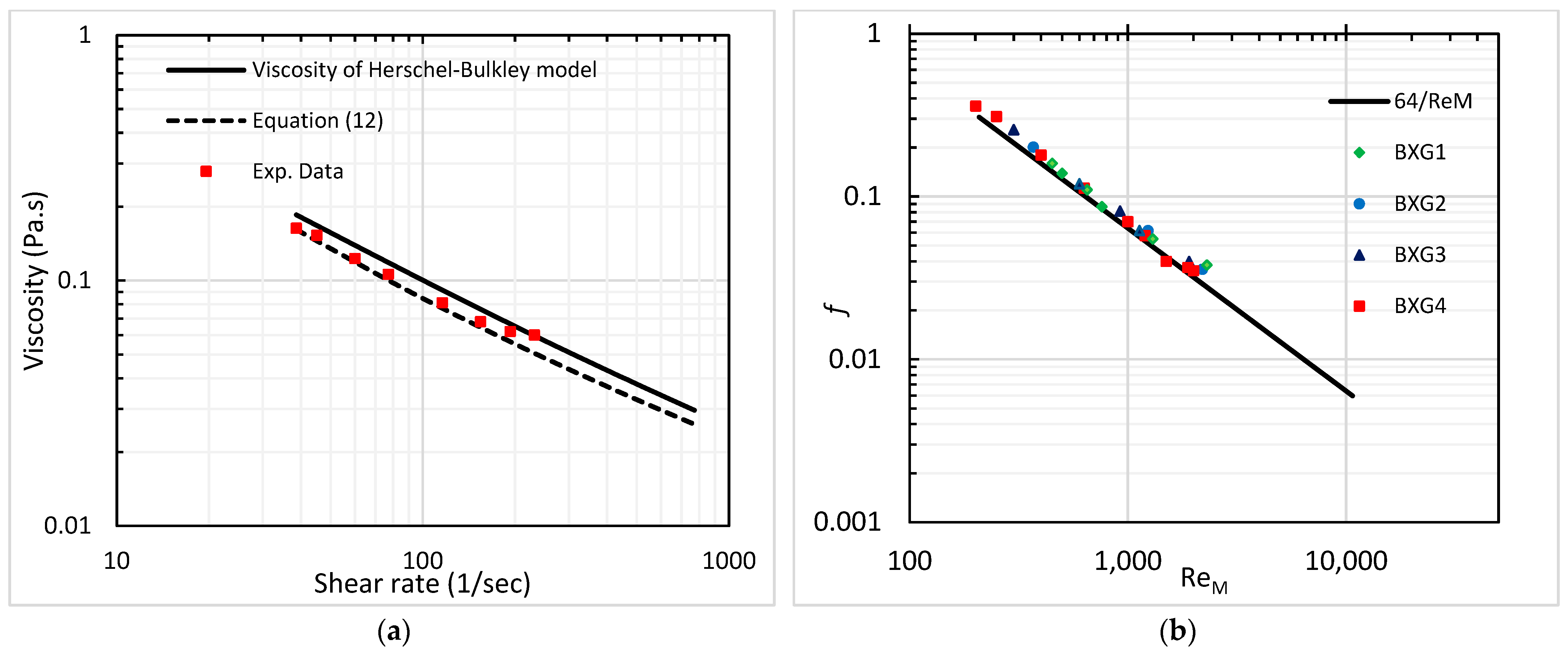
Figure 7 presents the experimental data of Herschel–Bulkley fluids in laminar flow. Figure 7a shows collated data in a log–log scale where the fluid viscosity obtained from the viscometer readings was depicted by the black solid curve. The dashed line represents the viscosity values calculated by the modified Equation (12) while disregarding the flow regime (laminar flow was assumed).
The modified equation provided a reasonable estimation of fluid viscosity for the laminar regions that matches the experimental results based on the Herschel–Bulkley rheological model. Additionally, it was noted that the calculated viscosity matched the modified laminar Herschel–Bulkley viscosity model until a certain point where a mismatch became apparent at transitional and turbulent flow regimes.
Figure 7b illustrates the laminar flow experimental data for four Herschel–Bulkley fluids (BXG1, BXG2, BXG3, and BXG4), which showed better values for the high yield effect in terms of error percentage than that of the calculated results.

4.10. Transitional Velocity Predictions

Critical velocity Vc or transitional velocity predictions were made for the Metzner and Reed method [20], the method with a modified Reynolds number by Slatter [21], and our modified method. These predictions were compared to the experimental critical velocity for each rheological model to evaluate the effect of changing the rheological parameters, to validate our improved method, and to evaluate the transitional velocity of Herschel–Bulkley fluids. The average percentage error of prediction models was compared to the experimental results. The experimental critical velocities versus the prediction for CMC1; high-concentration CMC4 for the power-law model; and BXG1, BXG2, and BXG4 for the Herschel–Bulkley model are shown in Table 3. The Metzner and Reed [20] method was found to be in good agreement with the experimental results when using power-law fluids, with an overpredicting of critical velocity by an average error of 6.4% in both diameters. The average error was found to decrease with an increased concentration of CMC by 4.6%. Slatter [21] predicted the transitional velocity of Herschel–Bulkley fluids to be most accurate when the effect of yield stress is small with an average underprediction of 5.1%. At higher yield stress fluid, errors increased by 7.6%. The developed method that considered the effective inner diameter of the pipe and yield region of Herschel–Bulkley fluid was compared to the experimental data. This model gives an average overprediction of the transitional velocity of 5.5% at minor effect yield stress. Using BXG4 fluid with high dominated yield stress resulted in an average of 6.1%. This model provides a reasonable estimate of fluid viscosity up to transitional regions and matches the calculation of the Herschel–Bulkley fluid exceptionally well.

4.11. Turbulent Flow Predictions

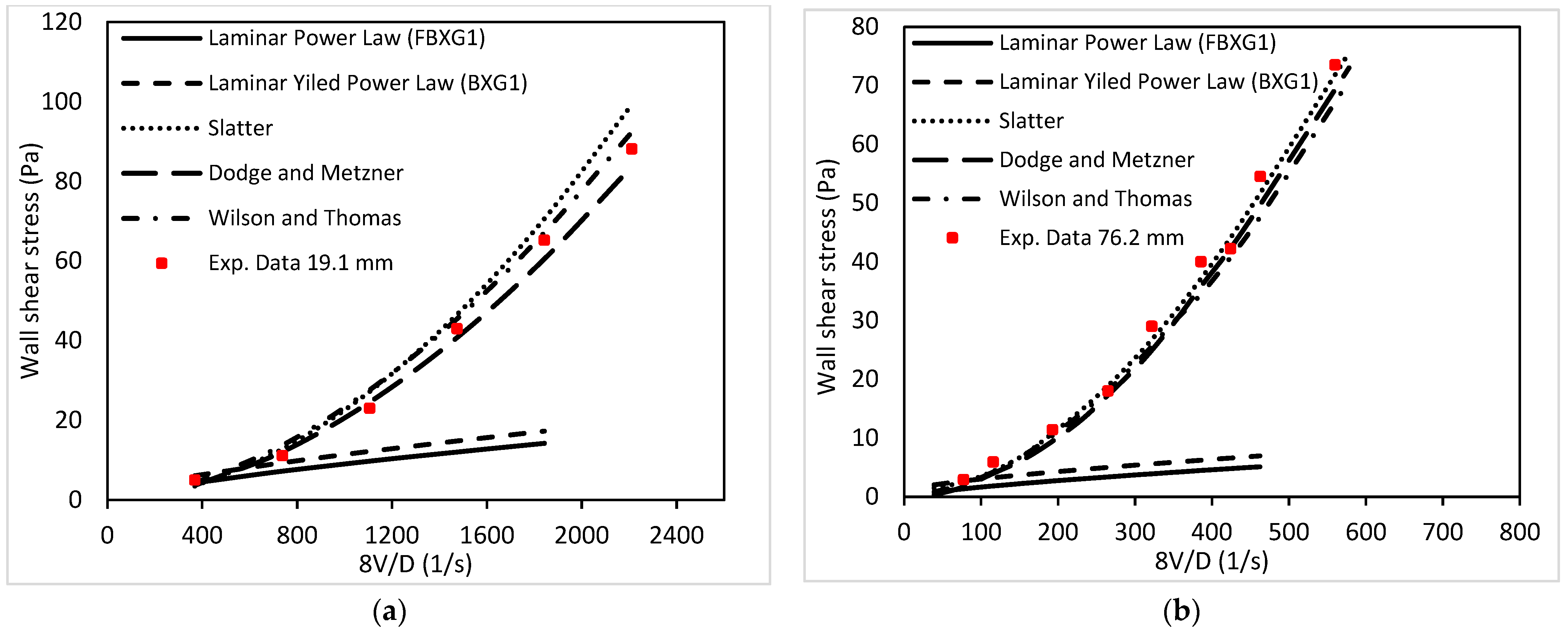
The experimental results from each pipe were compared to the turbulent prediction models of Slatter [21], Wilson and Thomas [26], and Dodge and Metzner [27] and presented on plots of shear stress τw against 8V/D in both laminar and turbulent conditions. The average absolute error was used to estimate and rank turbulent flow predictions to the experimental values.
The experimental results and prediction models in Ø19.1 and Ø76.2 mm diameters for power-law FBXG1 and Herschel–Bulkley fluid BXG1 are shown in Figure 8. Using the power-law model for FBXG1, the Dodge and Metzner [23] method gave accurate predictions for a small diameter with an average error of 2.6%. For a large diameter, it gave an underprediction by a mean absolute relative error of 2.5% (Figure 8a). With an increase in pipe diameter, the mean absolute relative error increased by 3.32%. However, the Wilson and Thomas [22] method gave overpredicted turbulent experimental data with a mean absolute relative error of 4.15% in a small diameter. It gave an underprediction at a 76.2 mm diameter by a mean absolute relative error of 5.86% when choosing power-law behaviour for FBXG1 fluid (Figure 8b). The experimental turbulent flow data points were compared to the theoretical prediction made by Slatter’s [21] model when choosing Herschel–Bulkley behaviour for BXG1 fluid. The evaluated turbulent flow model gave an overprediction in the small loop with a mean absolute relative error of 7.7%, and it was an underestimate of experimental results with a mean absolute relative error of 2.9% in a 76.2 mm diameter flow loop. The Slatter model considered his adoptive concept of the affected boundary layer from particle roughness in a turbulent model. The choice of rheological model has a minimal effect on the estimation of pressure gradients when the fluid has the same rheological curve and low dominated yield stress.
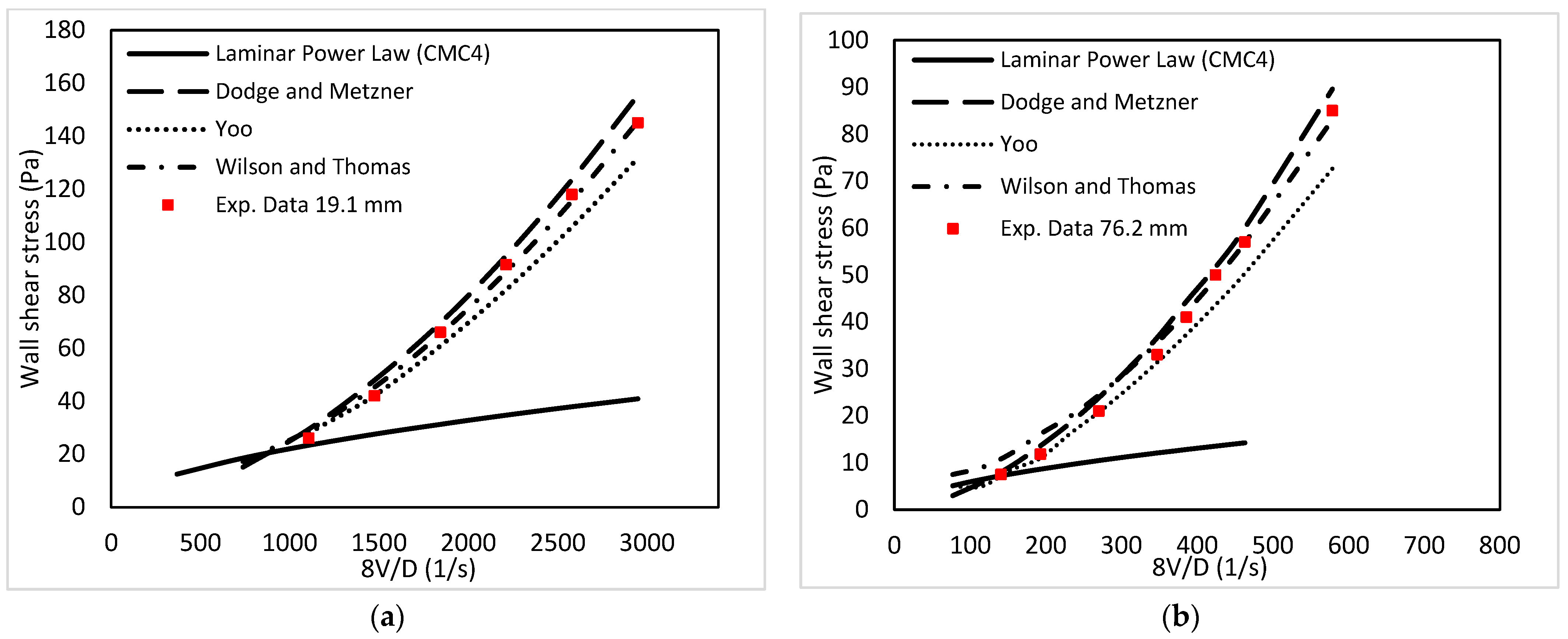
Figure 9 shows the experimental results and the predicted flow for the CMC4 power-law fluid. The Wilson and Thomas [26] method generated acceptable accuracy results for both small and large pipe sizes by a mean absolute relative error of 6.3% and 4.4%, respectively, especially for the high shear stress range. Dodge and Metzner [27] issued similar predictions for this fluid when using either small or large pipe diameters with a mean absolute relative error of 5.7–3.8% each across two pipe sizes, mainly at lower shear stress ranges. Estimations were also conducted by Yoo [29] on the correlation of turbulent flow for power-law fluids. Results obtained by Yoo in both diameters showed underprediction in terms of mean absolute relative error by 12 and 14%, respectively, which matched the shape of the experimental data at a lower shear stress range. Yoo’s model was unsuccessful in predicting, and it exhibited the greatest variability and deviation from the experimental results. Binxin Wu [57] made similar observations.
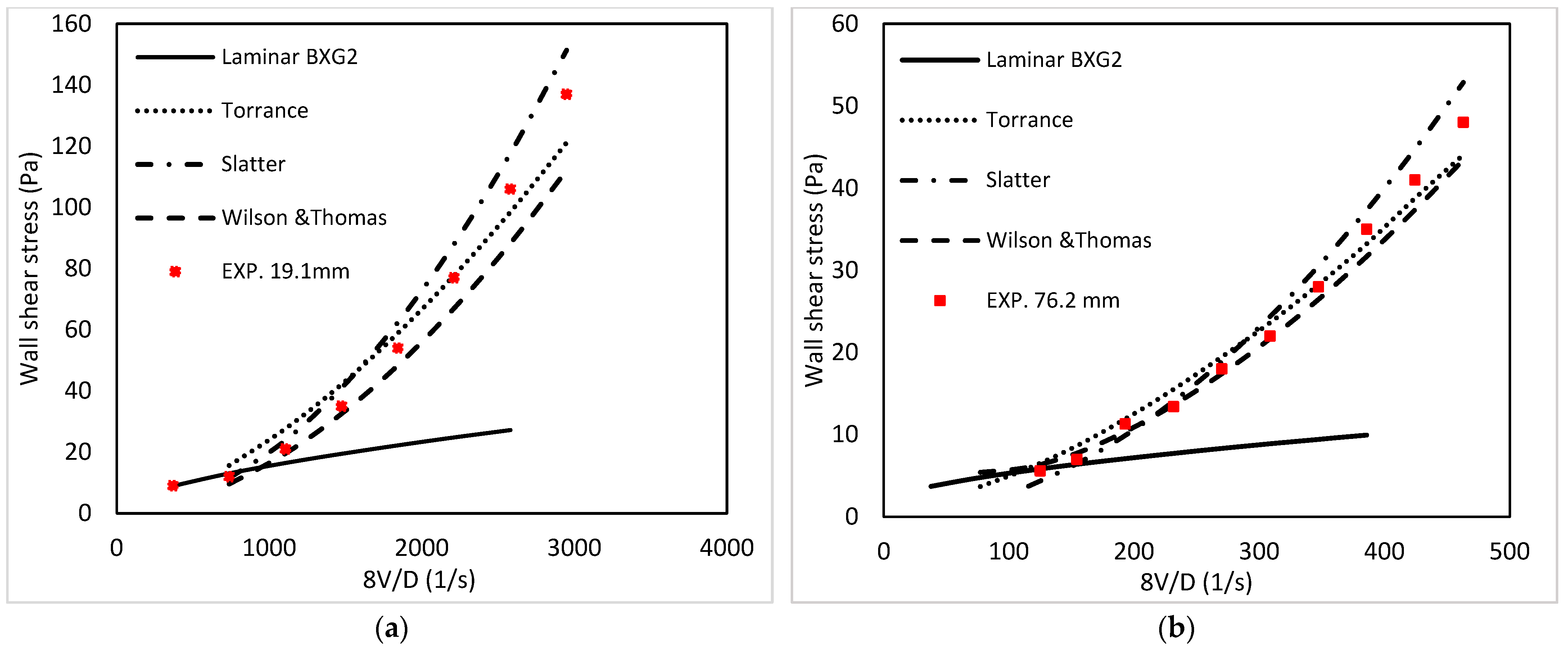
The theoretical predictions were compared to the experimental results of turbulent flow behaviour for Herschel–Bulkley fluids in Figure 10 and Figure 11 with two different rheology parameters in small and large pipe flow loops. When using the Herschel–Bulkley model, flow results for the BXG2 fluid are shown in Figure 10 for a pipe diameter of 19.1 mm (a) and a pipe diameter of 76.2 mm (b). Within the low effect of yield shear, the Slatter [21] method provided good estimates, while the accuracy increased with the increase in pipe diameter with a mean absolute relative error of 8.8% in Figure 10a and of 5.1% in Figure 10b.
The Wilson and Thomas [26] method gave underpredictions in both diameters: Ø19.1 mm and Ø76.2 mm. The error decreased as the pipe diameter increased, which followed the shape of the experimental data at a lower shear stress range with a mean absolute relative error of 11.2 and 8.7%, respectively, when using the Herschel–Bulkley model. The Torrance [28] method overpredicted at low turbulent shear stress for both small and larger pipe diameters, while it underpredicted at high effects of shear stress, and errors varied from 10.7% in a small diameter pipe to 8.6% in a large diameter pipe.
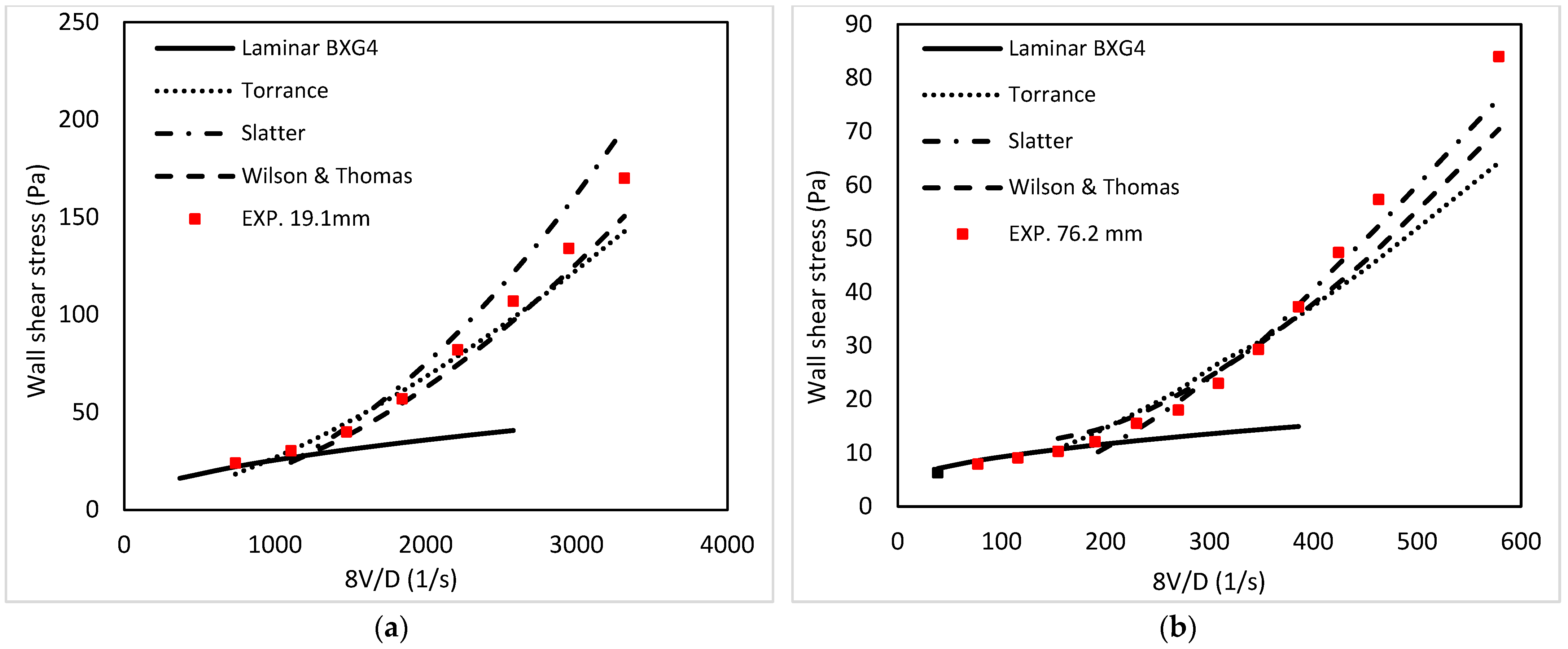
Regarding increased rheological parameters and the higher presence of yield stress, high-concentrated BXG4 experimental results and predictions are shown in Figure 11. The Wilson and Thomas [26] method resulted in an average underprediction of 8.9% in a small diameter pipe, which decreased as diameter increased with a mean absolute error of 7.3%.
The Torrance [28] model gave overpredicted experimental turbulent data at low shear stress and an underprediction at high shear with an average mean absolute relative error of 11.1% in the small diameter pipe. In contrast, the average error increased in a 76.2 mm diameter pipe by a mean absolute relative error of 13.5% due to the neglect of the effective yield shear rate. As shown in Figure 11, the Slatter [21] method generated acceptable accuracy results for both pipe sizes. This approach gave an overestimate in the small loop with a mean absolute relative error of 10.1% and an overestimate in the experimental results with a mean absolute relative error of 4.9% in a 76.2 mm diameter pipe.

4.12. Investigation of ANSYS Fluent Turbulence Models

The aim of this numerical study based on varying flow conditions was to assess the ability of CFD ANSYS Fluent in a turbulent model to simulate shear-thinning fluids, especially Herschel–Bulkley fluids, with the effect of yield stress. It also aimed to determine the effect of the selected rheological model on transport process efficiency by comparing the experimental pressure gradient to the CFD results.

4.13. Validation of Simulation Model

Calibration tests with water were performed prior to the beginning of shear-thinning fluid procedures to evaluate pressure loss. The experimental results were then compared to CFD ANSYS Fluent to assess the ability of those models to simulate Newtonian fluid (water) flows in two horizontal pipe sizes with a different wall function approach.
Two horizontal pipes of diameters 19.1 mm and 76.2 mm and a length of 8 m were used to examine six turbulence models for solving two transport equations that include three k-ε models (standard, RNG, and realizable k-ε) and three k-ω models (standard, BSL, and SST k-ω). A fine mesh was used to achieve mesh resolution near the pipe wall. Scalable wall functions were set for the k-ε models with y+ > 11.225 and y+ ~ 1 to 5 for the k-ω models to be able to resolve the viscous sublayer and buffer layer.
Table 4 shows ΔPCFD and the error indicator δ at two flow rates of water in a pipe with a diameter of 19.1 mm and two flow rates in a pipe with a diameter of 76.2 mm compared to our experimental results. In comparison to the collected experimental data, the CFD model replicated with good agreement, resulting in errors that varied from 2.2% to 9.3% and were larger for the small-diameter pipe. For turbulent Newtonian fluids, most of the RANS models coupled with the wall function approach successfully evaluated the pressure drop.

4.14. Evaluation of Turbulence Models for Shear-Thinning Fluids

CFD ANSYS Fluent simulations were performed in a steady-state regime. A second-order upwind approach was applied to maintain numerical stability. The RANS models k–ε and k–ω were used with the standard model constants. More details are given in [51].
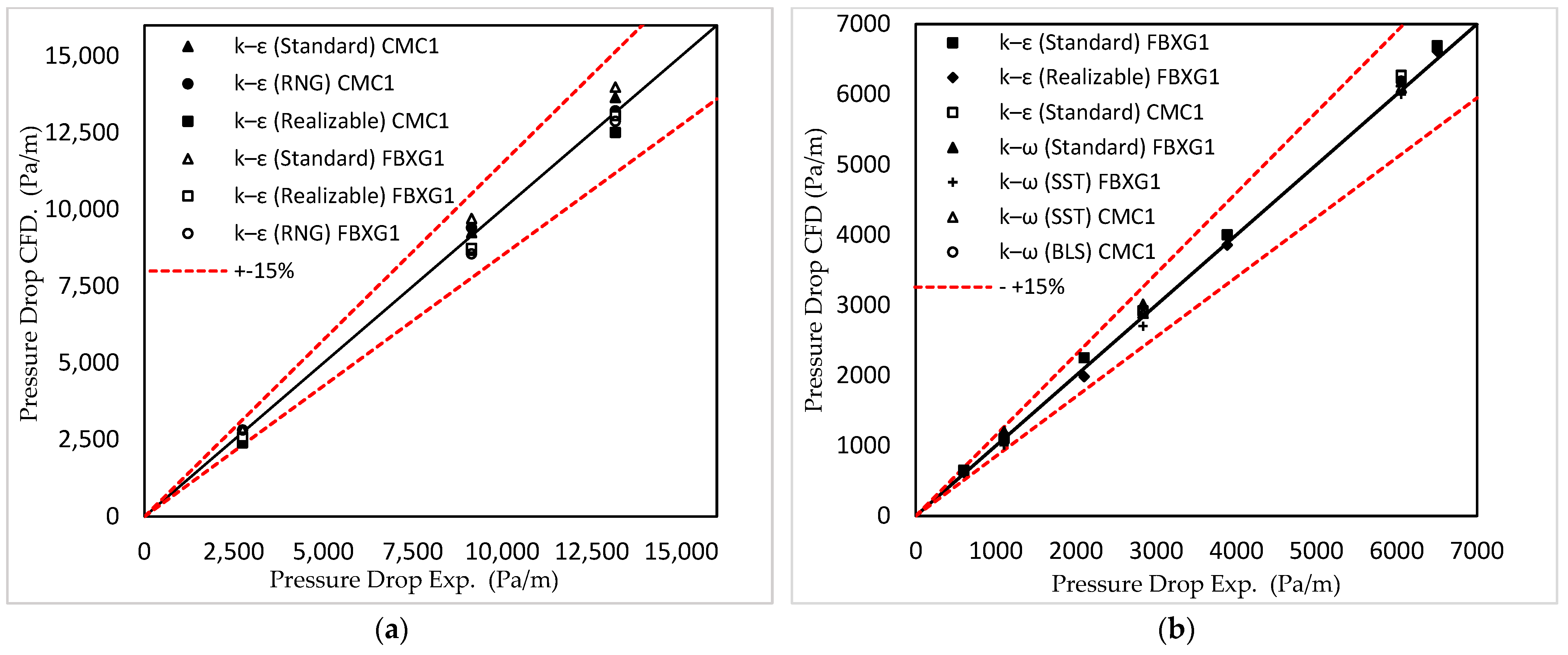
The comparison between the experimentally measured pressure gradient and the numerically predicted pressure gradient by CFD for power-law fluids (FBXG1 and CMC1) in different flow conditions are presented in Figure 12a for Ø19.1 mm and Figure 12b for Ø76.2 mm. Overall, this comparison demonstrated that all models could predict the pressure gradient in pipelines accurately at a low effect of viscosity. Both k-ω and k-ε gave high-precision underestimations by 5.8% to overestimations by 6.6% with an error margin of 15%, where all the measured points were within the indicated margin.
As a response to increasing CMC concentration, n decreased and k (rheological parameters) and viscosity of shear-thinning fluids increased. The experimental results and results from CFD predictions for power-law CMC4 fluid are shown in Figure 13. The comparison of CFD models showed that the k-ω and k-ε models were consistently overestimated in the small diameter (Figure 13a). The comparison also showed that the k-ω models had better results and standard deviation than the k-ε models. Furthermore, all models predicted the experimental results of CMC4 fluid with an error margin of less than 15%. The majority of data points were above 6.2% error, and the mean absolute error was determined at 6.9% to 13.5% for all models.
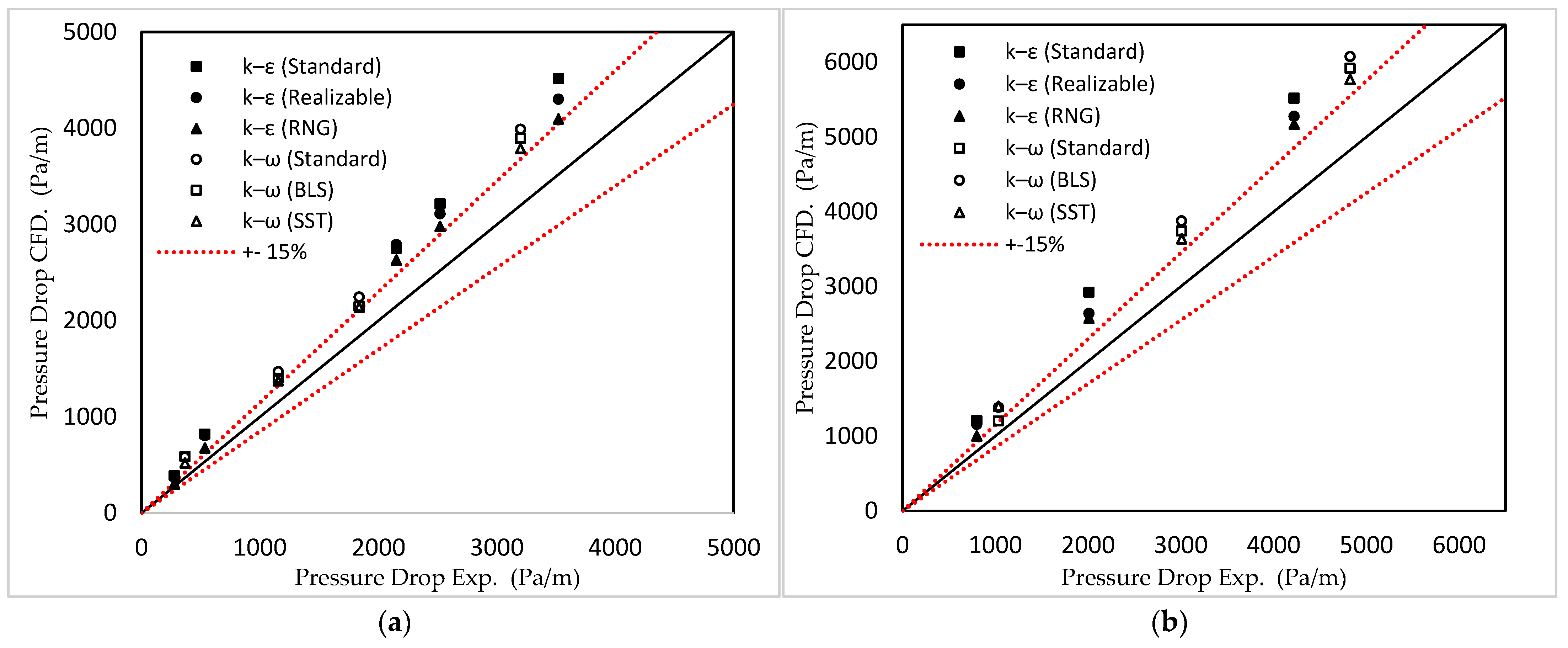
To investigate the effects of different yield stress values, simulations of shear-thinning Herschel–Bulkley fluids through two different pipe sizes were performed and presented in Figure 14. The Herschel–Bulkley fluid (BXG2) with a low effect of yield stress (1.92 Pa) in a pipe diameter of 19.1 mm is shown in Figure 14a, and BXG4 with a mild impact of yield stress (3.06 Pa) in a pipe diameter of 76.2 mm is shown in Figure 14b.
The comparison showed overprediction of the CFD results in Figure 14a for all k-ω models and k-ε models, especially at high flow rates. The k-ε renormalization group (RNG) and SST k-ω gave a better average absolute relative error than other models by 18.3% and 16.1%, respectively.
Figure 14b shows results for decreasing n, increasing k, and greater presence of yield stress (rheological parameters) of the highly concentrated BXG4 fluid CFD model compared with the experimental data. In comparison with three k-ω and three k-ε models, when the concentration and the pipe diameter increased, the mean absolute relative error increased. The k–ε (standard) gave an average absolute relative error of 25.1%, while k–ε (realizable) and k–ε (RNG) were overpredicted by 33.2% and 38.3%, respectively. The standard k-ε turbulence model did not count the drag reduction impact and could deliver unsatisfactory results and predictions in near-wall zones, where viscosity changed rapidly with distance from the pipe wall [58,59]. The k–ω (standard) and k–ω (BLS) were also overrated by 27.2% and 26.3%, respectively. The SST k-ω model had a low average absolute relative error of 20.1% when using BXG4 fluid. When compared to other models, the SST k-ω model performed better in the near-wall region. Such performance was important to consider, as shown in the next section.

4.15. Modified Viscosity Model

To show the obtained differences between the numerical predictions using the modified Papanastasiou [51] model and the standard Herschel–Bulkley viscosity model, the results obtained in two cases are shown in Figure 15.
The Papanastasiou-modified Herschel–Bulkley viscosity equation is not available in the library of CFD codes in ANSYS Fluent 19. A turbulence model was implemented using user-defined functions (UDFs). Papanastasiou’s modified viscosity equation was applied in the current CFD study. This modified viscosity function was shown to be numerically stabilized and devoid of discontinuity at a vanishing shear rate. Figure 15 shows a comparison between experimental data and measured CFD data for different yield stress values at the same pipe diameter. Figure 15a depicts a comparison between the experimental results of BXG2 Herschel–Bulkley fluid with a small effect of yield stress in the 76.2 mm pipe diameter and CFD-predicted results both by the standard Herschel–Bulkley viscosity model and by the modified Herschel–Bulkley–Papanastasiou viscosity model.
As observed in Figure 15a, the average absolute relative error decreased to 12.5% when using the SST k-ω model, especially in the transitional region. Moreover, the modified Herschel–Bulkley–Papanastasiou viscosity model gave better results in the transitional region. With increasing viscosity and yield stress effects (BXG4 fluid) (Figure 12b) the modified Herschel–Bulkley–Papanastasiou model CFD results showed an overprediction with an average absolute relative error within 16.1% when applying the SST k-ω model. The results from CFD data using the modified viscosity were better than those from CFD data using the normal Herschel–Bulkley viscosity model, which gave an average absolute relative error of 20.1%.
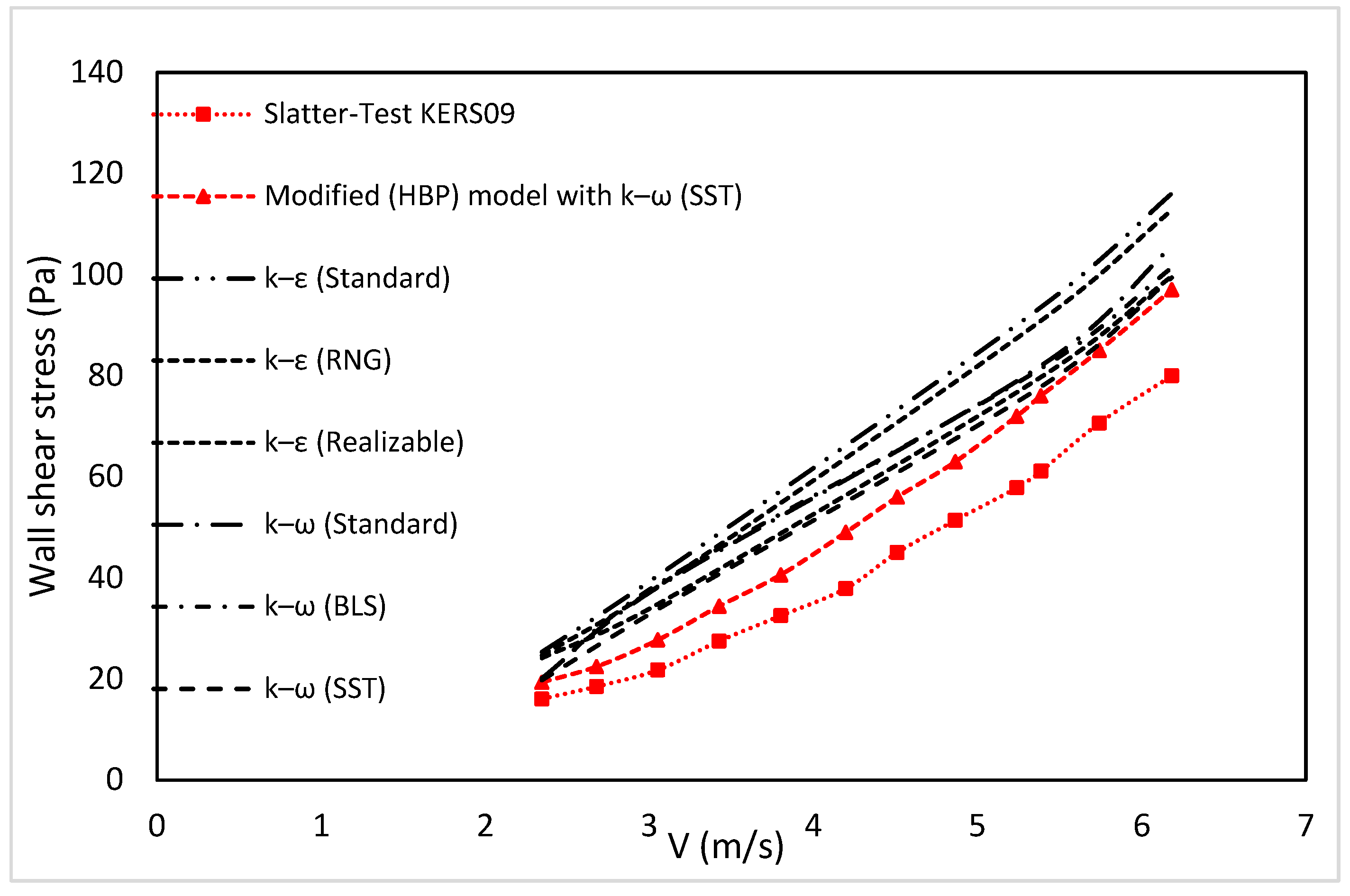
To investigate the effect of high yield stress of Herschel–Bulkley fluid, Figure 16 represents a KERS09 fluid, which had a very high yield stress effect, τy = 10.9 Pa. When using the standard Herschel–Bulkley viscosity model, the average absolute relative error was 30–57% in all k–ε and k–ω models. While using the Herschel–Bulkley–Papanastasiou viscosity model, the results of the SST k-ω model could reproduce the experimental results by an average absolute relative error of 22.3%. As shown in Figure 16, the regularization parameter δ in the rheological Herschel–Bulkley–Papanastasiou model was more effective in the transitional region, where  R e S T = 2628 to 4069.

5. Conclusions

This research helps to understand the properties of shear-thinning fluids in the engineering process through investigating their flow behaviour. The investigation was conducted experimentally and numerically using two different pipe diameters. The experimental data on the rheology and the pressure drop were the source for the collected experimental data, where two flow loops with smooth pipes were used to generate the data. The main conclusions of this study are summarized as follows:
The characteristics of the shear-thinning fluid flow including translational velocity and friction pressure gradient loss were measured using twelve explicit equations;
All models were statistically compared with the experimental results;
In power-law rheology models, Wilson and Thomas [26] and Dodge and Matzner [27] models were discovered to be the best-fit models to the experimental results up to 45,000 RMR. However, beyond this limit, the Wilson–Thomas model results were significantly different from that of the Dodge and Metzner [27] model;
For Herschel–Bulkley fluids, the modified Reynolds number Slatter model [21] was found to be the most accurate in predicting the critical velocity compared to the experimental results of this research and the modified model;
For laminar and transitional regions, Equation (12), which considered the effect of the plug region, provided a good agreement with the viscosity of the Herschel–Bulkley fluid;
The Herschel–Bulkley rheological model occasionally described the drilling fluid viscosity for low values of the shear rate;
The Slatter [21] model was found to be most accurate in predicting the critical velocity and pressure losses through all pipe sizes and across all flow regimes;
Predictions in turbulent pipe flow of Herschel–Bulkley fluid are superior with a specific rheological model. Using a different model could have a significant impact on predictions, particularly when the yield stress is high;
Most turbulent models in CFD, which were associated with wall functions, were successfully validated for Newtonian fluid turbulent flows;
When comparing numerical (ANSYS Fluent) k-ω models to the power-law fluid, more accurate results were observed with fluids that have a higher behaviour index. On the other hand, k-ε was observed to work better with fluids that have a value of behaviour index greater than 0.54;
When comparing numerical results of the Herschel–Bulkley fluid against the experimental results of this study, the percentile error was observed to increase with an increase in the yield stress (τy);
User-defined functions were implemented in the current ANSYS Fluent 19, where the modified viscosity function resulted in the best fit at the low shear rates experimentally and produced more stable and discontinuity-free results at vanishing shear rates numerically.

Author Contributions

Conceptualization, A.I.; methodology, A.I., A.A., M.A.R. and S.B.; investigation, experimental, and numerical simulations, A.I.; Writing—original draft, A.I.; Writing—reviewing and editing, A.I. and A.A. All authors have read and agreed to the published version of the manuscript.

Funding

This research received no external funding.

Data Availability Statement

Some data are not publicly available but can be provided upon request.

Acknowledgments

The authors are grateful to the Libyan Ministry of Higher Education and Scientific Research, Wadi Alshatti University-Libya, and Drilling Technology Laboratory (DTL) staff for their support.

Conflicts of Interest

The authors declare no conflict of interest.

Nomenclature

A = area (m2);
D = pipe diameter (m);
Deff = effect pipe diameter (m);
f = friction factor (- );
k = fluid consistency coefficient (Pa ·sn);
n = flow behaviour index (-);
Q = volumetric flow rate (m3/s);
R = Dp/2 is the radius of the plug region (m);
ReST = Slatter Reynolds number (-);
RMR = Metzner and Reed Reynolds number (-);
U* = shear velocity (m/s);
u = localized linear velocity at (r) value (m/s);
V = mean velocity (m/s);
VN = Newtonian mean velocity (m/s);
α* = area ratio (-);
γ = shear rate (s–1);
μ0 = apparent viscosity (Pa · s);
μ = Newtonian viscosity (Pa · s);
μeff = effect apparent viscosity (Pa · s);
ρ = density of fluid (kg/m3);
τ = shear stress (Pa);
τw = wall shear stress (Pa);
τy = yield stress (Pa);
δ  = Controls the exponential growth of stress, (-)
Ω = velocity profile blunting factor

References

  1. El-Nahhas, K.; Mostafa, N.H. Prediction of non-Newtonian turbulent flow behaviour by a Newtonian approach. In Proceedings of the 10th International Water Technology Conference, IWTC10, Alexandria, Egypt, 23–25 March 2006; pp. 479–490. [Google Scholar]
  2. Chhabra, R.P.; Richardson, J.F.; Flow, N.N. Applied Rheology: Engineering Applications; Butterworth-Heinemann: Oxford, UK, 2008. [Google Scholar]
  3. Rahman, K.M. Analysis of Drilling Fluid Rheology & Pressure Drop Modelling to Improve Drilling Efficiency. Master’s Thesis, Schulich School of Engineering, University of Calgary, Calgary, AB, Canada, 2018. [Google Scholar]
  4. Demirdal, B.; Cunha, J.C. Olefin-based synthetic-drilling-fluids volumetric behaviour under downhole conditions. SPE Drill. Complet. 2009, 24, 239–248. [Google Scholar] [CrossRef]
  5. Garvin, T.R.; Moore, P.L. A Rheometer for Evaluating Drilling Fluids at Elevated Temperatures. In Proceedings of the SPE 3062 Presented at the Fall Meeting of the Society of Petroleum Engineers of AIME, Houston, TX, USA, 4–7 October 1970. [Google Scholar]
  6. Minton, R.C.; Bern, P.A. Field Measurement and Analysis of Circulating System Pressure Drops with Low-Toxicity Oil-Based Drilling Fluids. In Proceedings of the SPE 17242 Presented at the SPE/IADC Drilling Conference, Dallas, TX, USA, 28 February–2 March 1988. [Google Scholar]
  7. De Wolfe, R.C.; Coffin, G.B.; Byrd, R.V. Effects of Temperature and Pressure on Rheology of Less Toxic Oil Muds. In Proceedings of the SPE 11892 Presented at Offshore Europe, Aberdeen, UK, 6–9 September 1983. [Google Scholar]
  8. American Petroleum Institute. Recommended Practice on the Rheology and Hydraulics of Oil Well Drilling Fluids. API RP 13D, 3rd ed.; American Petroleum Institute: Washington, DC, USA, 1995. [Google Scholar]
  9. Jim, F.; Young, S.; De Stefano, G.; Lee, J.; Guo, Q. Nanotechnology for oilfield applications-hype or reality. In SPE International Oilfield Nanotechnology Conference and Exhibition; One Petro: Richardson, TX, USA, 2012. [Google Scholar]
  10. Pinho, F.T.; Oliveira, P.J.; Miranda, J.P. Pressure losses in the laminar flow of shear-thinning power-law fluids across a sudden axisymmetric expansion. Int. J. Heat Fluid Flow 2003, 24, 747–761. [Google Scholar] [CrossRef]
  11. Anand, V.; David Jr, J.; Christov, I.C. Non-Newtonian fluid–structure interactions: Static response of a microchannel due to internal flow of a power-law fluid. J. Non-Newton. Fluid Mech. 2019, 264, 62–72. [Google Scholar] [CrossRef]
  12. Moukhtari, F.E.; Lecampion, B. A semi-infinite hydraulic fracture driven by a shear-thinning fluid. J. Fluid Mech. 2018, 838, 573–605. [Google Scholar] [CrossRef]
  13. Picchi, D.; Ullmann, A.; Brauner, N.; Poesio, P. Motion of a confined bubble in a shear-thinning liquid. J. Fluid Mech. 2021, 918, A7. [Google Scholar] [CrossRef]
  14. Klotz, J.A.; Brigham, W.E. To determine Herschel-Bulkley coefficients. J. Pet. Technol. 1998, 50, 80–81. [Google Scholar] [CrossRef]
  15. Kelessidis, V.C.; Maglione, R. Modelling rheological behaviour of bentonite suspensions as Casson and Robertson-Stiff fluids using Newtonian and true shear rates in Couette viscometry. Powder Technol. 2006, 168, 134–147. [Google Scholar] [CrossRef]
  16. Whorlow, R.W. Rheological Techniques; E. Horwood: Bristol, UK, 1980; ISBN 0470267364/9780470267363. [Google Scholar]
  17. Herschel, W.H.; Bulkley, R. Measurement of consistency as applied to rubber-benzene solutions. Proc. ASTM Part II 1926, 26, 621–629. [Google Scholar]
  18. Saramito, P. A new elastoviscoplastic model based on the Herschel–Bulkley viscoplastic model. J. Non-Newton. Fluid Mech. 2009, 158, 154–161. [Google Scholar] [CrossRef]
  19. Amoo, L.M.; Layi Fagbenle, R. Overview of non-Newtonian boundary layer flows and heat transfer. In Applications of Heat, Mass and Fluid Boundary Layers; Woodland Publishing: Salt Lake City, UT, USA, 2020; ISBN 9780128179499. [Google Scholar]
  20. Metzner, A.B.; Reed, J.C. Flow of non-Newtonian fluids—Correlation of the laminar, transition, and turbulent-flow regions. AIChE J. 1955, 1, 434–440. [Google Scholar] [CrossRef]
  21. Slatter, P.T. Transitional and Turbulent Flow of Non-Newtonian Slurries. Unpublished Ph.D. Thesis, University of Cape Town, Cape Town, South Africa, 1994. [Google Scholar]
  22. Kaczmarczyk, K.; Kruk, J.; Ptaszek, P.; Ptaszek, A. Pressure Drop Method as a Useful Tool for Detecting Rheological Properties of Non-Newtonian Fluids during Flow. Appl. Sci. 2021, 11, 6583. [Google Scholar] [CrossRef]
  23. Slatter, P.T. The role of the yield stress on the laminar/turbulent transition. In Proceedings of the 9th International Conference on Transport and Sedimentation of Solid Particles, Cracow, Poland, 2–5 September 1997; pp. 2–5. [Google Scholar]
  24. Hedström, B.O.A. Flow of plastic materials in pipes. Ind. Eng. Chem. 1952, 44, 652–656. [Google Scholar] [CrossRef]
  25. Vlasak, P.; Chara, Z. Laminar and turbulent flow experiments with yield-power-law slurries. Powder Technol. 1999, 104, 200–206. [Google Scholar] [CrossRef]
  26. Wilson, K.C.; Thomas, A.D. A new analysis of the turbulent flow of non-Newtonian fluids. Can. J. Chem. Eng. 1985, 63, 539–546. [Google Scholar] [CrossRef]
  27. Dodge, D.W.; Metzner, A.B. Turbulent flow of non-Newtonian systems. AIChE J. 1959, 5, 189–204. [Google Scholar] [CrossRef]
  28. Torrance, B. Friction factors for turbulent non-Newtonian fluid flow in circular pipes. S. Afr. Mech. Eng. 1963, 13, 89–91. [Google Scholar]
  29. Yoo, S.S. Heat Transfer and Friction Factors for Non-Newtonian Fluids in Turbulent Pipe Flow; University of Illinois at Chicago: Chicago, IL, USA, 1974. [Google Scholar]
  30. Brown, N.P.; Heywood, N.I. Slurry Handling: Design of Solid-Liquid Systems; Elsevier Science: London, UK, 1991. [Google Scholar]
  31. Clapp, R.M. Turbulent heat transfer in pseudoplastic non-Newtonian fluids. In International Developments of Heat Transfer Part III; The American Society of Mechanical Engineers: New York, NY, USA, 1961; pp. 652–661. [Google Scholar]
  32. Thomas, A.D.; Wilson, K.C. New analysis of non-newtonian turbulent flowndashyield-power-law fluids. Can. J. Chem. Eng. 1987, 65, 335–338. [Google Scholar] [CrossRef]
  33. Slatter, P.T.; Petersen, F.W.; Moodie, L. Rheological characterisation of mineral slurries using balanced beam tube viscometry. J. South. Afr. Inst. Min. Metall. 1998, 98, 165–170. [Google Scholar]
  34. Skelland, A.H.P. Non-Newtonian Flow and Heat Transfer (Book on Quantitative Relationships for Non-Newtonian Systems, Considering Classification and Fluid Behaviour of Materials with Anomalous Flow Properties); John Wiley and Sons, Inc.: New York, NY, USA, 1967; 469p. [Google Scholar]
  35. Steffe, J.F. Rheological Methods in Food Process Engineering; Freeman Press: Dallas, TX, USA, 1996. [Google Scholar]
  36. Van den Heever, E. Rheological Model Influence on Pipe Flow Predictions for Homogeneous Non-Newtonian Fluids. Master’s Thesis, Cape Peninsula University of Technology, Cape Town, South Africa, 2013. [Google Scholar]
  37. Lovato, S.; Keetels, G.H.; Toxopeus, S.L.; Settels, J.W. An eddy-viscosity model for turbulent flows of Herschel–Bulkley fluids. J. Non-Newton. Fluid Mech. 2022, 301, 104729. [Google Scholar] [CrossRef]
  38. Gavrilov, A.A.; Rudyak, V.Y. Reynolds-averaged modeling of turbulent flows of power-law fluids. J. Non-Newton. Fluid Mech. 2016, 227, 45–55. [Google Scholar] [CrossRef]
  39. Gavrilov, A.A.; Rudyak, V.Y. Direct numerical simulation of the turbulent flows of power-law fluids in a circular pipe. Thermophys. Aeromechanics 2016, 23, 473–486. [Google Scholar] [CrossRef]
  40. Stainsby, R.; Chilton, R.A. Prediction of pressure losses in turbulent non-Newtonian flows: Development and application of a hybrid theological model. In Bhr Group Conference Series Publication; Mechanical Engineering Publications Limited, 1996; Volume 20, pp. 21–40. [Google Scholar]
  41. Singh, R.; Ahmed, R.; Karami, H.; Nasser, M.; Hussein, I. CFD analysis of turbulent flow of power-law fluid in a partially blocked eccentric annulus. Energies 2021, 14, 731. [Google Scholar] [CrossRef]
  42. Ihmoudah, A.; Rahman, M.A.; Butt, S.D. CFD and experimental studies of yield power-law fluids in turbulent pipe flow. In International Conference on Offshore Mechanics and Arctic Engineering. Am. Soc. Mech. Eng. 2018, 51296, V008T11A012. [Google Scholar]
  43. Bartosik, A. Modification of k-ε model for slurry flow with the yield stress. In Proceedings of the 10th International Conference Numerical Methods in Laminar and Turbulent Flow, Swansea, UK, 28 July–1 August 1997; pp. 265–274. [Google Scholar]
  44. Bartosik, A.S.; Hill, K.B.; Shook, C.A. Numerical Modelling of Turbulent Bingham Flow. In Proceedings of the 9th International Conference Transport and Sedimentation of Solid Particles, Cracow, Poland, 2–5 September 1997; Agricultural University of Wroclaw: Wroclaw, Poland, 2002. Part 1. pp. 69–81. [Google Scholar]
  45. Launder, B.E.; Sharma, B.I. Application of the energy-dissipation model of turbulence to the calculation of flow near a spinning disc. Lett. Heat Mass Transf. 1974, 1, 131–137. [Google Scholar] [CrossRef]
  46. Bartosik, A.S. Influence of Rheological Parameters on Predictions of Bingham Slurry Flow. In Proceedings of the 11th International Conference Transport and Sedimentation of Solid Particles, Ghent, Belgium, 9–12 September 2002; Agricultural Academy of Wrocław: Wrocław, Poland, 2002; Volume 438, pp. 143–150. [Google Scholar]
  47. Cayeux, E.; Leulseged, A. The effect of thixotropy on pressure losses in a pipe. Energies 2020, 13, 6165. [Google Scholar] [CrossRef]
  48. Magnon, E.; Cayeux, E. Precise method to estimate the herschel-bulkley parameters from pipe rheometer measurements. Fluids 2021, 6, 157. [Google Scholar] [CrossRef]
  49. Saasen, A.; Ytrehus, J.D. Viscosity models for drilling fluids—Herschel-bulkley parameters and their use. Energies 2020, 13, 5271. [Google Scholar] [CrossRef]
  50. ANSYS FLUENT Theory Guide 15.0; ANSYS, Inc.: Canonsburg, PA, USA, 2013; Available online: http://www.ansys.com (accessed on 5 March 2023).
  51. Papanastasiou, T.C. Flows of materials with yield. J. Rheol. 1987, 31, 385–404. [Google Scholar] [CrossRef]
  52. Genić, S.; Arandjelović, I.; Kolendić, P.; Jarić, M.; Budimir, N.; Genić, V. A review of explicit approximations of Colebrook’s equation. FME Trans. 2011, 39, 67–71. [Google Scholar]
  53. García, F.; García, J.M.; García, R.; Joseph, D. Friction factor improved correlations for laminar and turbulent gas–liquid flow in horizontal pipelines. Int. J. Multiph. Flow 2007, 33, 1320–1336. [Google Scholar] [CrossRef]
  54. García, F.; García, R.; Padrino, J.C.; Mata, C.; Trallero, J.; Joseph, D. Power-law and composite power-law friction factor correlations for laminar and turbulent gas– liquid flow in horizontal pipelines. Int. J. Multiph. Flow 2003, 29, 1605–1624. [Google Scholar] [CrossRef]
  55. Ouyang, L. Single Phase and Multiphase Fluid Flow in Horizontal Wells. Ph.D. Thesis, Department of Petroleum Engineering, School of Earth Sciences, Stanford University, Stanford, CA, USA, 1998; 248p. [Google Scholar]
  56. Xiao, J.J.; Shonham, O.; Brill, J.P. A comprehensive mechanistic model for two-phase flow in pipelines. In Proceedings of the 65th SPE Annual Technical Conference and Exhibition, Paper SPE 20631, New Orleans, LA, USA, 23–26 September 1990; pp. 167–180. [Google Scholar]
  57. Wu, B. Computational fluid dynamics investigation of turbulence models for non-Newtonian fluid flow in anaerobic digesters. Environ. Sci. Technol. 2010, 44, 8989–8995. [Google Scholar] [CrossRef]
  58. Mathur, A.; He, S. Performance and implementation of the Launder–Sharma low-Reynolds number turbulence model. Comput. Fluids 2013, 79, 134–139. [Google Scholar] [CrossRef]
  59. Versteeg, H.K.; Malalasekera, W. An Introduction to Computational Fluid Dynamics: The Finite Volume Method; Pearson Education: London, UK, 2007. [Google Scholar]
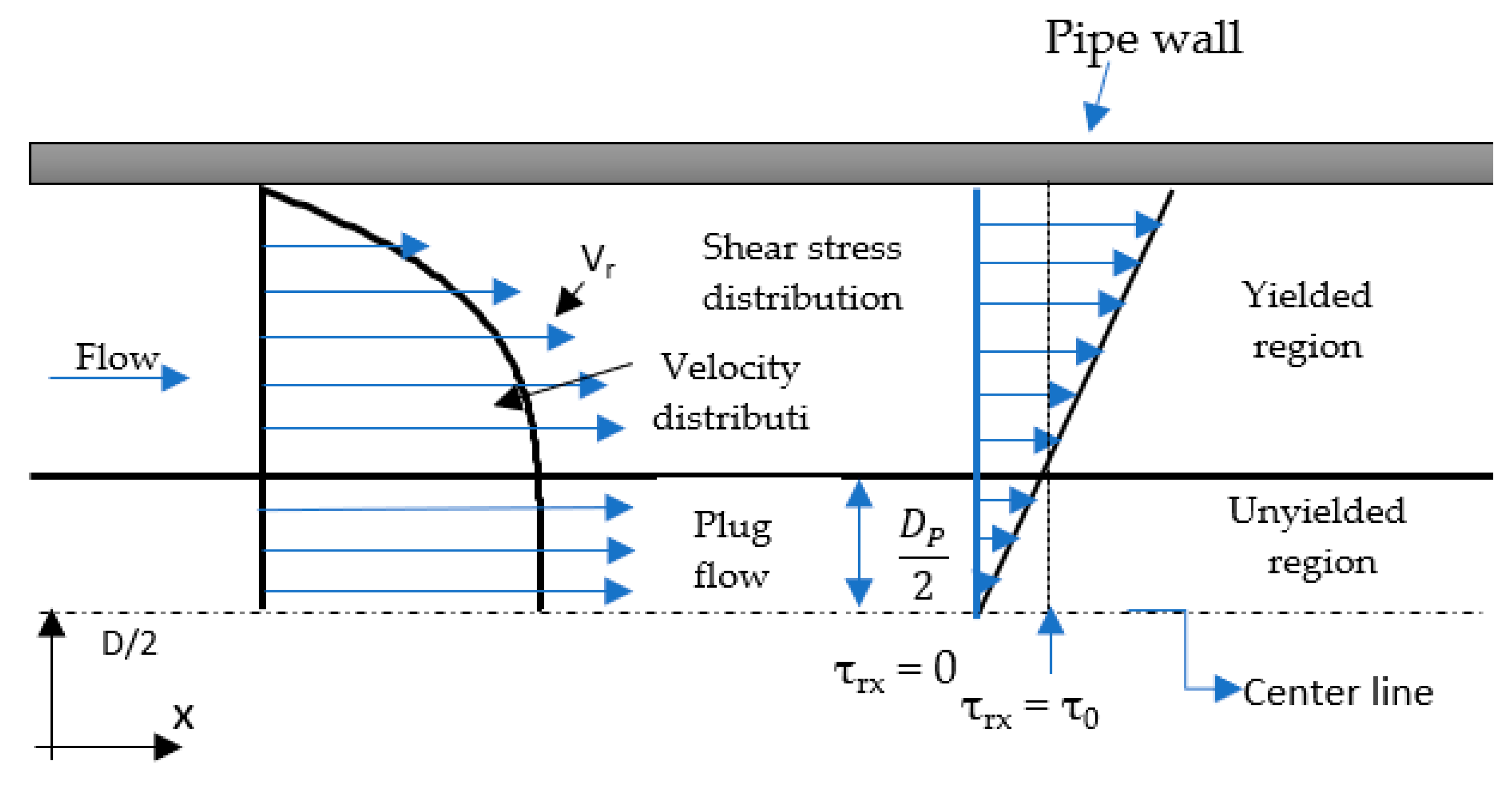
Figure 1. Velocity distribution in fully developed laminar flow for Herschel–Bulkley fluid in a circular pipe.
Energies 16 03478 g001
Figure 2. Experimental setup components and flow loops system. (a) Clear PVC open-loop re-circulating pipe with a diameter of 0.0762 m and a total length of 65 m. (b) PVC pipe with a diameter of 0.0191 m and a length of 22 m.
Energies 16 03478 g002
Figure 3. Shear stress vs. shear rate curves for non-Newtonian models. (a) Rheological curves of power-law model fit. (b) Rheological curves of Herschel–Bulkley model fit.
Energies 16 03478 g003
Figure 4. Shear stress vs. shear rate for BXG4 fluid according to the exponential model proposed by Papanastasiou [51].
Energies 16 03478 g004
Figure 5. The grid structure in the computational domain.
Energies 16 03478 g005
Figure 6. Grid independence study for Newtonian and shear-thinning fluids. (a) Water in pipe diameter 76.2 mm for k-ω models. (b) BXG4 (Herschel–Bulkley fluid) in pipe diameter 76.2 mm for k-ω models.
Energies 16 03478 g006
Figure 7. Comparison of the predicted and experimental data for Herschel–Bulkley fluids in pipe diameter 76.2 mm. (a) Estimated and experimental viscosity vs. Herschel–Bulkley viscosity for polymer solutions BXG4. (b) Laminar data of Herschel–Bulkley fluids (BXG1, BXG2, BXG3, and BXG4).
Energies 16 03478 g007
Figure 8. Comparison between predictions and experimental data of turbulent flow for low-concentrated FBXG1, BXG1 power-law fluids, and BXG1 Herschel–Bulkley fluids: (a) pipe diameter 19.1 mm, (b) pipe diameter 76.2 mm.
Energies 16 03478 g008
Figure 9. Comparison between predictions and experimental data of turbulent flow for high-concentrated CMC4 power-law fluid: (a) pipe diameter 19.1 mm, (b) pipe diameter 76.2 mm.
Energies 16 03478 g009
Figure 10. Comparison between predictions and experimental data of turbulent flow for BXG2 Herschel–Bulkley fluids: (a) pipe diameter 19.1 mm, (b) pipe diameter 76.2 mm.
Energies 16 03478 g010
Figure 11. Comparison between predicted and experimental data of turbulent flow for BXG4 Herschel–Bulkley fluids: (a) pipe diameter 19.1 mm, (b) pipe diameter 76.2 mm.
Energies 16 03478 g011
Figure 12. Comparison of frictional pressure drop obtained from CFD model vs. experimental data. (a) FBXG1 and CMC1 power-law fluids pipe diameter 19.1 mm. (b) FBXG1 and CMC1 power-law fluids pipe diameter 76.2 mm.
Energies 16 03478 g012
Figure 13. Comparison of frictional pressure drops obtained from CFD model vs. experimental data. (a) CMC4 power-law fluid pipe diameter 19.1 mm. (b) CMC4 power-law fluids pipe diameter 76.2 mm.
Energies 16 03478 g013
Figure 14. Comparison of frictional pressure drop obtained from CFD model vs. experimental data for Herschel–Bulkley fluids. (a) BXG2 fluid in pipe diameter 19.1 mm. (b) BXG4 fluid in pipe diameter 76.2 mm.
Energies 16 03478 g014
Figure 15. Comparison of pressure drop between experimental data and simulation results for standard and modified Herschel-Bulkley viscosity models: (a) BXG2 fluid in pipe diameter 19.1 mm, (b) BXG4 fluid in pipe diameter 76.2 mm.
Energies 16 03478 g015
Figure 16. Comparison of frictional pressure drop obtained from CFD model vs. experimental data for KERS09 Herschel–Bulkley law fluids.
Energies 16 03478 g016
Table 1. Mesh properties.
Statistics Newtonian SystemNewtonian System
Pipek-εk-ωk-εk-ω
DiameterModelsModelsModelsModels
Number of 76.2 mm2,680,5643,206,3863,826,8914,874,284
elements19.1 mm1,763,5922,153,4912,617,3302,771,148
Average 76.2 mm0.99120.99530.99590.9975
orthogonality19.1 mm0.99230.99660.99710.9985
Average 76.2 mm0.08060.05850.02610.0154
skewness19.1 mm0.06410.05110.01930.0106
Table 2. The curve-fitted parameters for shear-thinning fluid models are based on the rotational viscometer (Model 800), and KERS09 fluid came from experimental work provided by Slatter [21].
Compositions (gr/350 mL) Rheological Parameters
SymbolBentoniteXanthan Gum CMC   ρ  (kg/m3) nK (Pa.sn)τy (Pa)R2 (YPL Model)R2 (PL Model)
BXG15.52010100.740.05120.760.991-
BXG25.53010150.610.2411.920.992-
BXG45.54010250.560.4153.060.999-
CMC1--210000.720.06010-0.992
CMC2--310020.600.2330-0.994
CMC4--410050.570.4050-0.999
FBXG15.52010100.530.2210-0.985
KERS09Kaolin11310.8380.016210.7 Slatter [21]
Table 3. Transitional velocity model evaluation.
Diameter (mm)Power-Law Fluids—Metzner and Reed Herschel–Bulkley Fluids—Slatter
Exp. Critical Velocity (m/s)CMC1Exp.
Critical Velocity (m/s)
CMC4Exp. Critical Velocity (m/s)BXG1Exp. Critical Velocity (m/s)BXG2Exp.
Critical Velocity (m/s)
BXG4
19.1 mm1.191.212.152.281.040.961.651.552.222.03
7.5%6.1%−5.7%−7.8%−8.5%
76.2 mm0.560.591.241.280.70.671.010.961.631.52
5.3%3.2%−4.2%−5.2%−6.7%
Average6.4% 4.6% −5.1% −6.5% −7.6%
Developed model results
19.1 mm 1.041.111.651.742.222.42
6.7%5.4%7.2%
76.2 mm 0.70.731.011.041.631.71
4.2%2.4%4.9%
Average 5.5% 4.2% 6.1%
Table 4. Comparison between experimental results and CFD-predicted pressure gradient.
Large-Diameter PipeSmall-Diameter Pipe
Q = 100 L/minQ = 1000 L/minQ = 15 L/minQ = 60 L/min
PCFD (Pa/m)δ (%)PCFD (Pa/m)δ (%)PCFD (Pa/m)δ (%)PCFD (Pa/m)δ (%)
k–εStandard21.73.11349.23.7520.4−5.26152.9−3.1
RNG21.83.31381.06.1519.1−5.46151.5−3.2
Realizable20.6-2.61384.06.4497.5−9.45936.6−6.5
k–ωStandard22.14.81369.05.2591.77.76752.26.3
BSL22.35.51396.07.3600.29.36763.66.5
SST21.62.21335.02.6570.43.96498.52.3
Disclaimer/Publisher’s Note: The statements, opinions and data contained in all publications are solely those of the individual author(s) and contributor(s) and not of MDPI and/or the editor(s). MDPI and/or the editor(s) disclaim responsibility for any injury to people or property resulting from any ideas, methods, instructions or products referred to in the content.