Determination of Heat and Mass Transport Correlations for Hollow Membrane Distillation Modules

Abstract

Development and optimization of the membrane distillation (MD) process are strongly associated with better understanding of heat and mass transport across the membrane. The current state-of-the-art on heat and mass transport in MD greatly relies upon the use of various empirical correlations for the Nusselt number (Nu), tortuosity factor (τ), and thermal conductivity (${\kappa }_m$) of the membrane. However, the current literature lacks investigations about finding the most representative combination of these three parameters for modeling transport phenomena in MD. In this study, we investigated 189 combinations of Nu, ${\kappa }_m$, and τ to assess their capability to predict the experimental flux and outlet temperatures of feed and permeate streams for hollow fiber MD modules. It was concluded that 31 out of 189 tested combinations could predict the experimental flux with reasonable accuracy (R² > 0.95). Most of the combinations capable of predicting the flux reasonably well could predict the feed outlet temperature well; however, the capability of the tested combinations to predict the permeate outlet temperatures was poor, and only 13 combinations reasonably predicted the experimental temperature. As a generally observed tendency, it was noted that in the best-performing models, most of the correlations used for the determination of ${\kappa }_m$ were parallel models. The study also identified the best-performing combinations to simultaneously predict flux, feed, and permeate outlet temperatures. Thus, it was noted that the best model to simultaneously predict flux, feed, and permeate outlet temperatures consisted of the following correlations for τ, Nu, and ${\kappa }_m$: $=\frac{\epsilon }{1-{\left(1-\epsilon \right)}^{1/3}}$, $Nu=0.13{\left(Re\right)}^{0.64}{\left(Pr\right)}^{0.38}$, ${\kappa }_m=\left(1-\epsilon \right){\kappa }_{pol}+\epsilon {\kappa }_{air}$ where ε, Re, Pr, ${\kappa }_{pol}$, and ${\kappa }_{air}$ represent membrane porosity, Reynolds number, Prandtl number, thermal conductivities of polymer and air, respectively.

1. Introduction

Membrane distillation (MD) is a thermally driven process where the driving force is a vapor pressure difference created by a temperature difference across a porous hydrophobic membrane. MD can use low-grade heat from different sources, such as the sun, geothermal wells, and industrial processes, to produce ultra-fresh water [1,2,3]. MD is also an interesting candidate to achieve zero liquid discharge and crystallization from different solutions due to its ability to treat highly concentrated solutions, such as brine from desalination facilities [4,5,6,7]. The use of MD for simultaneous recovery of freshwater and minerals from different sources of impaired water makes it relevant to achieving sustainability and a circular economy [6,8].

MD can be operated in several configurations, including air gap, vacuum, sweep gas, and direct contact. Direct contact membrane distillation (DCMD) is the simplest configuration of the process in terms of the equipment and modules involved [9,10,11]. In DCMD, the membrane is in direct contact with the feed solution on one side and with the permeate on the other side. The driving force (i.e., vapor pressure difference) is induced by keeping the feed solution at a higher temperature than the permeate stream, creating a positive heat transfer through the membrane. Water and volatile compounds from the liquid feed evaporate, travel through the membrane pores, and are condensed at the membrane surface on the permeate side.

In DCMD, heat is transferred from the feed side to the permeate side due to the transport of water vapor through the membrane pores and conduction through the membrane [12,13]. As a result, the temperature at the membrane surface differs from its value in the bulk of the solution. The mass (vapor) flux across the membrane is directly linked with the difference in vapor pressures at the membrane surface on the feed and permeate sides, where the mass transfer coefficient of the membrane appears as a constant. The temperature difference between the bulk solution and membrane surface is known as temperature polarization, which decreases the effective driving force across the membrane and results in a reduction in transmembrane vapor flux [13]. The mass transfer coefficient of the membrane is a function of membrane properties including pore size, overall porosity, thickness, and the τ which, depending upon the membrane pore size and mean free path of the water vapor, can be calculated according to different models [3]. Determination of the vapor pressure at the surface requires knowledge of the membrane surface temperatures, which are linked with the bulk temperatures through heat transfer coefficients [14]. The thermal conductivity of the membrane (${\kappa }_m$) affects the heat conducted across the membrane and therefore directly influences the total heat transport across the membrane and hence the temperature at the membrane surface [15]. Thus, the determination of flux is associated with the calculation of surface temperatures and the mass transfer coefficient of the membrane.

Understanding heat and mass transport in MD is important to design, improve, and optimize the process and module design [3,16,17,18]. Numerous semi-empirical correlations have been proposed to calculate the Nusselt number (Nu) for heat transfer coefficient in MD channels (see Section 2.3) [13,19]. The ultimate selection of the correlation for the Nu for a given fluid is a function of the applied hydrodynamics and the system configuration (e.g., flat sheet, hollow fiber). Likewise, Nu, several correlations have been proposed to describe the ${\kappa }_m$, including the parallel resistance model, the series resistance model, and the Maxwell I model, as described in Section 2.3. In all these correlations, effective membrane thermal conductivity models account for the membrane porosity, the thermal conductivity of stagnant air within the pore, and the thermal conductivity of the membrane material. High ${\kappa }_m$ decreases the temperature gradient across the membrane, which results in lower vapor flux [20]. For τ, which is inversely linked with the vapor flux, three different approaches have been adopted [21,22]: (i) use it as an adjustable parameter in the model; (ii) use a constant value (usually between 1 and 2, but occasionally greater than 2) for the τ; and (iii) use theoretical approaches to link the membrane porosity with the τ.

Despite their fundamental importance, heat and mass transport in MD are poorly understood [13,23,24]. The current state-of-the-art modeling of MD approaches has two major limitations regarding the use of various correlations for the Nu, ${\kappa }_m$, and τ of the membrane. Firstly, they compare the validity of various correlations proposed for any of the three parameters (Nu, τ, and ${\kappa }_m$) for a fixed combination of the other two parameters. In other words, the state-of-the-art approaches do not test the validity of various combinations of correlations for the Nu, ${\kappa }_m$, and τ of the membrane. For instance, in some studies for the determination of a suitable correlation for the Nu, it was assumed that the ${\kappa }_m$ could be represented by the parallel model [13,25]. Phattaranawik et al. considered the suitability of ${\kappa }_m$ correlations in their DCMD model but neglected the correlations for τ [26]. Kim et al. studied the effect of using eleven different correlations for the τ on the flux and concluded that the use of an inappropriate correlation can incorporate a significant error in the predicted flux [27]. However, the study was carried out by assuming that heat transport within the membrane and in feed and permeate channels can be described by using a fixed combination of correlations for ${\kappa }_m$ and Nu. This approach is clearly very specific to the membrane and operating setup applied in each of the studies, and its validity for a broad set of membrane and module characteristics cannot be guaranteed. The second important limitation of the current state-of-the-art is that the validation of different correlations for Nu, ${\kappa }_m$, and τ has been tested by comparing the theoretical and experimental values of vapor flux only [11,15,27,28,29]. The potential of these models to predict the outlet temperatures of feed and permeate, which are crucial to calculating thermal and cooling energy demand, respectively, is broadly neglected in the current literature.

The overall objective of the current study is to analyze the capability of various combinations of state-of-the-art correlations for Nu, ${\kappa }_m$, and τ to predict the experimental flux and outlet temperatures for hollow fiber membrane modules. The ultimate objective is to find the best-suited combination of Nu, ${\kappa }_m$, and τ to predict the experimental data (flux and outlet temperatures).

2. Materials and Methods

2.1. MD Test

Experimental analysis of DCMD has been conducted to validate the model predictions by using a polypropylene hollow fiber membrane from Membrana GmbH. The membrane has a porosity of 73%, a mean pore size of 0.2 µm, and a thickness of 450 µm. The membrane module, consisting of 19 hollow fibers with an effective length of 51 cm placed in a shell with a 2.1 cm internal diameter, was fabricated in the laboratory. The experiments were performed with pure water as feed and permeate circulating on the lumen and shell sides, respectively, of the hollow fiber membrane module operating in the countercurrent mode. The Reynolds numbers for the permeate and feed sides were in the ranges 130–300 and 200–1800, respectively. Inlet and outlet temperatures of the feed and permeate streams were measured by using thermocouples (TECPEL thermometers). The flux was measured by following the weight loss of the feed container as a function of experimental time. Circulation of hot and cold streams was achieved by using a peristaltic pump (Masterflex L/S). The temperatures of the feed and permeate streams were controlled by using heating (Grant) and cooling (Julabo 200F) systems, respectively. Detailed experimental design parameters can be found in Table 1, whereas a schematic illustration of the experimental setup can be found elsewhere [30,31,32]. The experimentation was designed to comprehend the effect of different operating parameters, including feed inlet temperature and feed and permeate flow rates, on the process performance.

Table 1. Experimental temperatures and flow rates used in the study.

No.	Feed Inlet Temperature (°C)	Permeate Inlet Temperature (°C)	Feed Flow Rate (Lh−1)	Permeate Flow Rate (Lh−1)
1	35	12	99	29
2	39	13	99	29
3	44	14	99	29
4	48	15	99	29
5	49	18	99	29
6	49	22	99	29
7	57	17	99	29
8	65	16	99	29
9	48	14	68	29
10	48	14	43	29
11	47	14	29	29
12	49	14	99	23
13	48	15	99	32
14	48	15	99	50

2.2. Model Development

Mass flux in MD can be described mathematically as follows:

$$J=B(P_{fm}-P_{pm})$$

(1)

where P_fm and P_pm are the vapor pressures at the membrane surface on the feed and permeate sides, respectively. B is a characteristic membrane parameter, and different models can be used to determine it [3]. The ultimate selection of the model depends on the mean free path of the water vapor and the nominal pore size of the membrane. For PP hollow fiber membranes, the mean free path of water molecules and the nominal pore size are in the same order of magnitude [20,33], and thus the combined Knudsen- and molecular diffusion model is used to determine B (see Equation (2)).

$$B={\left[\frac{3\tau {\delta }_m}{2\epsilon r}{\left(\frac{\pi R{T}_m}{8M}\right)}^{\frac{1}{2}}+\frac{\tau {\delta }_m{P}_{air}R{T}_m}{\epsilon P_{tot}DM}\right]}^{-1}$$

(2)

P_air is the air pressure, and P_tot is the total pressure inside the membrane [3]. τ can be described by different correlations, as detailed in Section 2.3. D is the vapor diffusivity and is affected by both the temperature and P_tot. An empirical correlation between P_tot and D is proposed in a study by Yun et al. [4] (see Equation (3)) and is used in our study.

$$P_{tot}D=1.19\cdot {10}^{-4}\cdot T^{1.75}$$

(3)

To estimate the mass flux over the membrane, the difference in vapor pressure at the two membrane surfaces must be known. The vapor pressure is described as a function of temperature in the Antoine equation (see Equation (4)) [5]. Therefore, temperature on the membrane surfaces in the feed (T_fm) and permeate (T_pm) is a prerequisite for the calculation of P_fm and P_pm.

$$P=\exp \left(A_a-\frac{B_a}{T+C_a}\right)$$

(4)

Since mass flux is driven by a temperature gradient between the feed and permeate streams, an accurate calculation of the heat transfer across the membrane must be applied. Heat transfer in MD can be divided into three steps [6]:

• Heat transfer from the feed bulk to the membrane surface with the rate Q_f;
• Heat transfer across the membrane with the rate Q_m;
• Heat transfer from the boundary layer to the bulk solution on the permeate side is at a rate of Q_p.

Both the heat transfer in the permeate and feed solutions are convection processes and thus dependent upon a convective heat transfer coefficient ($h_{f/p}$) and the temperature polarization according to Equations (5) and (6) [34]:

$$Q_f=h_f(T_f-T_{fm})$$

(5)

$$Q_p=h_p(T_{pm}-T_p)$$

(6)

The heat transfer coefficient in the feed and permeate solution can be estimated from the following correlation between Nu, the thermal conductivity of the solution ${\kappa }_{p/f}$, and the equivalent diameter $D_e$ of the channel (see Equation (7)).

$$h_{p/f}=\frac{N{u}_{p/f}{\cdot \kappa }_{p/f}}{D_e}$$

(7)

The equivalent diameter corresponds to the diameter of the fibers in the solution on the lumen side. For the solution on the shell side, Equation (8) should be used due to the triangular arrangement of the fibers [7]. Furthermore, multiple empirical correlations have been proposed to determine Nu. Thus, to ensure the most accurate prediction of the flux, different Nu correlations are investigated in this study (see Section 2.3) [14].

$$D_e=\frac{3.44\cdot P_t^2-\pi {\cdot d}_{out}^2}{\pi \cdot d_{out}}$$

(8)

$d_{out}$ is the outer diameter of the fibers, and $P_t$ is the average distance between the centers of the fibers [7].

The heat transfer rate across the membrane is affected by the ${\kappa }_m$ and the mass transfer across the membrane (see Equation (9)) [35].

$$Q_m=\frac{{\kappa }_m}{{\delta }_m}\left(T_{fm}-T_{pm}\right)+J\mathsf{\Delta }{H}_v=h_c\left(T_{fm}-T_{pm}\right)+h_v\left(T_{fm}-T_{pm}\right)$$

(9)

where ${\kappa }_m$ can be calculated according to different correlations relating the thermal conductivity of the polymer used as membrane material, ${\kappa }_{pol}$ and the thermal conductivity of the air, ${\kappa }_{air}$, present in the pores, as detailed in Section 2.3 [6]. ${\delta }_m$ is the thickness of the membrane, and $\mathsf{\Delta }{H}_v$ is the latent heat of water vapor, which is dependent on the temperature at the membrane surfaces (see Equation (10))

$$\mathsf{\Delta }{H}_v=1.7535\left(\frac{T_{fm}+T_{pm}}{2}+2024.3\right)$$

(10)

Under the steady state conditions:

$$Q_f=Q_m=Q_p$$

(11)

Due to the equality of the different heat transfer rates at steady state, the following correlations between T_fm, T_pm, T_f, and T_p can be derived [3].

$$T_{fm}=T_f-(T_f-T_p)\frac{\frac{1}{h_f}}{\frac{1}{h_v+h_c}+\frac{1}{h_p}+\frac{1}{h_f}}$$

(12)

$$T_{pm}=T_p+(T_f-T_p)\frac{\frac{1}{h_p}}{\frac{1}{h_v+h_c}+\frac{1}{h_p}+\frac{1}{h_f}}$$

(13)

To calculate the temperature profile along the module, the energy balance along the fibers must be applied. This is done by dividing the system into (L/n) elements, where L is the total length of the system and n is the total number of elements. The energy difference between the entrance and exit on the feed side for the i-th element is equal to the amount of energy transferred across the membrane due to conduction and convection (see Equations (14) and (15)), with a corresponding correlation also applicable for the permeate stream [3]. Thus, the feed and permeate temperatures for element i + 1 along the fiber for the countercurrent configuration can be calculated as follows:

$$T_{f{|}_{i+1}}=\frac{\dot{m_f}{C}_p{T}_{f{|}_i}-\left(\frac{{\kappa }_m}{{\delta }_m}\left(T_{fm}-T_{pm}\right)dA+J\mathsf{\Delta }{H}_{v}dA\right)}{\dot{m_f}{C}_{p{|}_{i+1}}}$$

(14)

$$T_{p{|}_{i+1}}=\frac{\dot{m_p}{C}_p{T}_{p{|}_i}-\left(\frac{{\kappa }_m}{{\delta }_m}\left(T_{fm}-T_{pm}\right)dA+J\mathsf{\Delta }{H}_{v}dA\right)+Q_e}{\dot{m_p}{C}_{p{|}_{i+1}}}$$

(15)

Calculating temperature profiles along the module length allows for the determination of mass transfer both parallel to the flow and across the membrane in discrete steps. This is simply calculated as the difference of mass flux along the module and across the membrane of the previous element:

$${\dot{m}}_{f{|}_{i+1}}={\dot{m}}_{f{|}_i}-J_{i}dA$$

(16)

The heat transfer to the environment (Q_e in Equation (18)) is firstly governed by the convective heat transfer from the bulk solution on the shell side to the inner surface of the module with a rate Q_inner, and secondly by the conductive heat transfer across the module with a rate Q_module. Lastly, heat is transferred from the outer surface of the module to the environment via both convection with the rate Q_outer and radiation with the rate Q_r. The formula for the different rates is presented in Equation (17) [8].

$$\begin{gathered} Q_{inner}=h_{inner}{A}_{inner}\left(T_{bulk}-T_{s,inner}\right) \\ {Q}_{module}=\frac{k_{module}}{{\delta }_{tube}}{A}_m\left(T_{s,inner}-T_{s,outer}\right) \\ {Q}_{outer}=h_{outer}{A}_{outer}\left(T_{s,outer}-T_{air}\right) \\ {Q}_r=A_{outer}Cϵ\left(T_{s,outer}^4-T_{air}^4\right) \end{gathered}$$

(17)

At steady state, the following equality for the heat loss can be applied.

$$Q_e=Q_{in}=Q_{module}=Q_{out}+Q_r$$

(18)

2.3. Variable Parameters

Three parameters used for the modeling computations are varied, i.e., τ, ${\kappa }_m$, and Nu. Nine correlations for the Nu, seven for τ, and three for the ${\kappa }_m$ are tested. The specific details about the correlations used are presented in Table 2. All possible combinations of the considered correlations are tested, i.e., 189 combinations in total. Nu correlations are empirically determined and depend on various dimensionless parameters, module length, and equivalent diameter. The correlations presented in the table are valid in the laminar flow regime, i.e., Re < 2100. Considered correlations for ${\kappa }_m$ are the parallel resistance model, the series resistance model, and the Maxwell I model [8].

Table 2. Correlations of $\tau$, Nu, and ${\kappa }_m$ used in the DCMD computations.

Tortuosity $\left(\mathit{\tau }\right)$
${\mathit{\tau }}_{\mathbf{1}}=\frac{{\left(\mathbf{2}-\mathit{\epsilon }\right)}^{\mathbf{2}}}{\mathit{\epsilon }}$	[27]
${\mathit{\tau }}_{\mathbf{2}}=\frac{\mathit{\epsilon }}{\mathbf{1}-{\left(\mathbf{1}-\mathit{\epsilon }\right)}^{\mathbf{1}\mathbf{/}\mathbf{3}}}$	[28]
${\mathit{\tau }}_{\mathbf{3}}=\frac{\mathbf{1}}{\sqrt{\mathit{\epsilon }}}$	[30]
${\mathit{\tau }}_{\mathbf{4}}=\frac{\mathbf{1}}{\mathit{\epsilon }}$	[27]
${\mathit{\tau }}_{\mathbf{5}}=\frac{\left(\mathbf{3}-\mathit{\epsilon }\right)}{\mathbf{2}}$	[30]
${\mathit{\tau }}_{\mathbf{6}}=\sqrt{\mathbf{1}-\mathit{l}\mathit{n}\left(\mathit{\epsilon }/\mathbf{2}\right)}$	[30]
${\mathit{\tau }}_{\mathbf{7}}=\frac{\mathit{\epsilon }}{\mathbf{1}-{\left(\mathbf{1}-\mathit{\epsilon }\right)}^{\mathbf{2}/\mathbf{3}}}$	[30]
Nusselt number ($\mathit{N}\mathit{u}$)
$\mathit{N}{\mathit{u}}_{\mathbf{1}}=\mathbf{1.86}{\left(\frac{\mathit{R}\mathit{e}\mathit{P}\mathit{r}}{\mathit{L}/{\mathit{D}}_{\mathit{e}}}\right)}^{\mathbf{1}/\mathbf{3}}$	[31]
$\mathit{N}{\mathit{u}}_{\mathbf{2}}=\mathbf{4.36}\left(\frac{\mathbf{0.036}\mathit{R}\mathit{e}\mathit{P}\mathit{r}\left({\mathit{D}}_{\mathit{e}}/\mathit{L}\right)}{\mathbf{1} + \mathbf{0.0011}\mathit{R}\mathit{e}\mathit{P}\mathit{r}{\left({\mathit{D}}_{\mathit{e}}/\mathit{L}\right)}^{\mathbf{0.8}}}\right)$	[31]
$\mathit{N}{\mathit{u}}_{\mathbf{3}}=\mathbf{0.13}{\left(\mathit{R}\mathit{e}\right)}^{\mathbf{0.64}}{\left(\mathit{P}\mathit{r}\right)}^{\mathbf{0.37}}$	[32]
$\mathit{N}{\mathit{u}}_{\mathbf{4}}=\mathbf{1.95}{\left(\frac{\mathit{R}\mathit{e}\mathit{P}\mathit{r}}{\mathit{L}/{\mathit{D}}_{\mathit{e}}}\right)}^{\mathbf{1}/\mathbf{3}}$	[33]
$\mathit{N}{\mathit{u}}_{\mathbf{5}}=\mathbf{0.097}{\left(\mathit{R}\mathit{e}\right)}^{\mathbf{0.73}}{\left(\mathit{P}\mathit{r}\right)}^{\mathbf{0.13}}$	[34]
$\mathit{N}{\mathit{u}}_{\mathbf{6}}=\mathbf{3.66}+\left(\frac{\mathbf{0.104}\mathit{R}\mathit{e}\mathit{P}\mathit{r}\left({\mathit{D}}_{\mathit{e}}/\mathit{L}\right)}{\mathbf{1} + \mathbf{0.106}\mathit{R}\mathit{e}\mathit{P}\mathit{r}{\left({\mathit{D}}_{\mathit{e}}/\mathit{L}\right)}^{\mathbf{0.8}}}\right)$	[33]
$\mathit{N}{\mathit{u}}_{\mathbf{7}}=\mathbf{1.62}{\left(\mathit{R}\mathit{e}\mathit{P}\mathit{r}{\mathit{D}}_{\mathit{e}}/\mathit{L}\right)}^{\mathbf{0.33}}$	[35]
$\mathit{N}{\mathit{u}}_{\mathbf{8}}=\mathbf{4.36}+\frac{\mathbf{0.023}\mathit{P}\mathit{e}/\left(\mathit{L}/{\mathit{D}}_{\mathit{e}}\right)}{\mathbf{1} + \mathbf{0.0012}\mathit{P}\mathit{e}/\left(\mathit{L}/{\mathit{D}}_{\mathit{e}}\right)}$	[36]
$\mathit{N}{\mathit{u}}_{\mathbf{9}}=\mathbf{4.364}+\frac{\mathbf{0.02633}}{\left(\mathit{L}/{\left({\mathit{D}}_{\mathit{e}}\mathit{P}\mathit{e}\right)}^{\mathbf{0.506}}\right)\mathbf{exp}\left(\mathbf{41}\mathit{L}/\left({\mathit{D}}_{\mathit{e}}\mathit{P}\mathit{e}\right)\right)}{\left(\frac{\mathit{P}\mathit{r}}{\mathit{P}{\mathit{r}}_{\mathit{w}}}\right)}^{\mathit{k}}$ $\mathit{k}=\mathbf{0.20}$—feed, $\mathit{k}=\mathbf{0.19}$—permeate	[36]
Membrane thermal conductivity $\left({\mathit{\kappa }}_{\mathit{m}}\right)$
${\mathit{\kappa }}_{\mathit{m},\mathbf{1}}=\left(\mathbf{1}-\mathit{\epsilon }\right){\mathit{\kappa }}_{\mathit{p}\mathit{o}\mathit{l}}+\mathit{\epsilon }{\mathit{\kappa }}_{\mathit{a}\mathit{i}\mathit{r}}$	[37]
${\mathit{\kappa }}_{\mathit{m},\mathbf{2}}={\left(\frac{\mathit{\epsilon }}{{\mathit{\kappa }}_{\mathit{a}\mathit{i}\mathit{r}}}+\frac{\mathbf{1}-\mathit{\epsilon }}{{\mathit{\kappa }}_{\mathit{p}\mathit{o}\mathit{l}}}\right)}^{-\mathbf{1}}$	[37]
${\mathit{\kappa }}_{\mathit{m},\mathbf{3}}={\mathit{\kappa }}_{\mathit{a}\mathit{i}\mathit{r}}\left(\frac{\mathbf{1} + \left(\mathbf{1}-\mathit{\epsilon }\right)\mathbf{2}{\mathit{\beta }}_{\mathit{p}\mathit{o}\mathit{l}-\mathit{a}\mathit{i}\mathit{r}}}{\mathbf{1}-\left(\mathbf{1}-\mathit{\epsilon }\right)\mathbf{2}{\mathit{\beta }}_{\mathit{p}\mathit{o}\mathit{l}-\mathit{a}\mathit{i}\mathit{r}}}\right)$${\mathit{\beta }}_{\mathit{p}\mathit{o}\mathit{l}-\mathit{a}\mathit{i}\mathit{r}}=\left({\mathit{\kappa }}_{\mathit{p}\mathit{o}\mathit{l}}-{\mathit{\kappa }}_{\mathit{a}\mathit{i}\mathit{r}}\right)/\left({\mathit{\kappa }}_{\mathit{p}\mathit{o}\mathit{l}}+\mathbf{2}{\mathit{\kappa }}_{\mathit{a}\mathit{i}\mathit{r}}\right)$	[37]

3. Results and Discussion

3.1. Experimental Mass Fluxes and Outlet Temperatures

Details of experimental input (inlet temperatures and flow rates) and output (outlet temperatures and fluxes) parameters are provided in Table 3. It is evident from the table that the flux increases with an increase in feed temperatures and flow rates. Experiments 1–8 indicate that flux increases exponentially from 1.05 to 6.07 kg/m².h by increasing the feed temperature from 35 to 65 °C at a constant feed and permeate flow rate. This agrees with the exponential dependence of flux on temperature in MD reported in the literature [3,36]. The corresponding feed outlet temperature also increases, from 34 to 60 °C. A similar trend is also observed for the permeate outlet temperature. Experiments 9–11 were aimed at investigating the effect of feed flow rate on transmembrane flux and outlet temperatures. It is evident from the corresponding data that the flux decreases with the feed flow rate. This is a direct consequence of increased temperature polarization and feed temperature drop along the membrane module, as evident from the corresponding T_fout data. The observed trend again corresponds to the observations reported in the literature [37]. Experiments 12–14 were carried out to explore the effect of permeate flow rates on the mass flux and temperature drops along the module. As evident from the corresponding flux data reported in Table 3, flux exhibits a very weak dependence upon the permeate flow rate. Both feed and permeate outlet temperatures drop slightly with an increase in permeate flow rate, which was expected due to improved heat transfer on the permeate side and a shorter residence time for the permeate stream inside the module.

Table 3. Experimentally measured inlet and outlet temperatures and trans-membrane flux at known feed and permeate temperatures and flow rates.

No.	Tf,in [°C]	Tf,out [°C]	Tp,in [°C]	Tp,out [°C]	Qf [L/h]	Qp [L/h]	J [kg m−2h−1]
1	35	34	12	18	99	29	1.05
2	39	38	13	20	99	29	1.35
3	44	42	14	21	99	29	1.84
4	48	46	15	24	99	29	2.35
5	49	47	18	27	99	29	2.27
6	49	47	22	29	99	29	2.38
7	57	54	17	29	99	29	3.76
8	65	60	16	32	99	29	6.07
9	48	42	14	23	68	29	2.13
10	48	42	14	23	43	29	2.15
11	47	38	14	22	29	29	1.84
12	49	47	14	25	99	23	2.45
13	48	47	15	23	99	32	2.43
14	48	46	15	22	99	50	2.48

3.2. Evaluation of the Model Predictions

All possible combinations of Nu, κ_m, and τ shown in Figure 1 have been evaluated to assess their ability to predict the experimental values of the average flux across the membrane and the outlet temperatures T_f,out and T_p,out. The accuracy of the results is determined by the R²-value of the fit to the function y = x of the experimental (y) and model prediction (x) data. Detailed results are shown in Table A1 in the Appendix A, which indicates that the R² values for flux and outlet temperatures predicted by each of the combinations differ widely. Thus, R²-values for J fall in the interval −2.866 < R² < 0.989, while R² values for T_f,out and T_p,out lie in the intervals 0.891 < R² < 0.977 and −0.529 < R² < 0.969, respectively. The variation of R²-values across all models is noteworthy, as it indicates that model predictions are significantly affected by the combination of the adjustable parameters used.

Figure 1. An illustration of different combinations of k_m, τ, and Nu tested in the study. The numbering for each correlation is according to Table 2.

A statistical analysis of the data has been provided in Figure 2. It is evident from Figure 2 that only 31 out of 189 combinations could predict the flux with accuracy exceeding R² > 0.9. This emphasizes the significance of using the appropriate combination of tortuosity, heat transfer, and ${\kappa }_m$ correlations in DCMD modeling. Furthermore, the variation and the number of low R²-values suggest that many combinations yield inaccurate predictions. Thus, evaluation of the prediction performance of a given model may have to account for the relative model performance rather than the absolute performance. The number of combinations that could predict T_f,out with R² > 0.9 was the highest (180). On the other hand, only 13 combinations could predict T_p,out with reasonable accuracy (R² > 0.9).

Figure 2. Statistical analysis of different combinations of Nu, τ, and κ_m used to predict the experimental parameters.

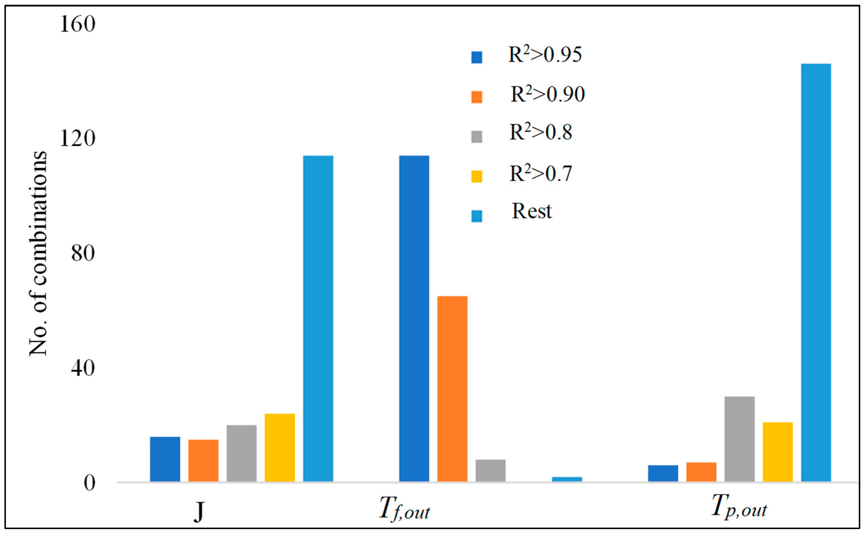
3.3. Selection of the Best Fitting Model

The selection of the best-fitting model in this study is based on the highest sum of the R²-values for J, T_f,out, and T_p,out. The combinations of the three adjustable parameters τ, Nu, and ${\kappa }_m$ with the best overall prediction performance based on the conditions set in this study are reported in Table 4 along with the corresponding R²-values. The accuracy of the fit to flux, feed, and permeate outlet temperatures is represented with R²(J), R²(T_f,out), and R²(T_p,out), respectively. R²_tot is the average of R²(J), R²(T_f,out), and R²(T_p,out).

Table 4. R²-values and correlation numbers (numbers for τ, Nu, and κ_m correspond to Table 3) for the best-fitting model (based on fit for T_f,out, T_p,out, and J).

τ	Nu	${\mathit{\kappa }}_{\mathit{m}}$	${\mathit{R}}^2\left(\mathit{J}\right)$	${\mathit{R}}^2\left({\mathit{T}}_{\mathit{f},\mathit{o}\mathit{u}\mathit{t}}\right)$	${\mathit{R}}^2\left({\mathit{T}}_{\mathit{p},\mathit{o}\mathit{u}\mathit{t}}\right)$	${\mathit{R}}_{\mathit{t}\mathit{o}\mathit{t}}^2$
2	3	1	0.970	0.976	0.951	0.966
1	3	1	0.911	0.976	0.948	0.945
2	5	1	0.951	0.973	0.907	0.944
1	5	1	0.880	0.973	0.903	0.918
6	9	1	0.942	0.970	0.805	0.906

The model with the best predictability for all the parameters is the one that combines τ₂, Nu₃, and ${\kappa }_{m,1}$. The experimental values are plotted against the predicted values for this model in Figure 3 to confirm the model’s performance. It is evident from the figure that the model predicts all three parameters well, but standard deviations vary between J, T_f,out, and T_p,out, where J-standard deviations are generally higher than those of T_p,out and especially T_f,out.

Figure 3. Model using τ₂, Nu₃, and κ_m,1. (a) Experimental versus predicted J (both axes are on a logarithmic scale of base 10); (b) experimental vs. predicted T_f,out; and (c) experimental vs. predicted T_p,out. Note that error bars in some cases are smaller than the points and, therefore, are not visible for some points.

One may note from Table A1 that the model with the best overall prediction ability does not have the best prediction ability when solely focusing on the flux. Therefore, it is necessary to investigate the best model when only taking flux prediction into account. Several combinations of τ, Nu, and ${\kappa }_m$ can determine the flux accurately. The best five models for flux prediction are shown in Table 5 along with their corresponding R² values for their general predictions. It is evident from the table that even though a given model can predict the flux well, this does not necessarily entail that it is also able to predict the outlet temperatures well.

Table 5. R²-values and correlation numbers (numbers for τ, Nu, and ${\kappa }_m$ correspond to Table 3) for the best-fitting model for the flux.

τ	Nu	${\mathit{\kappa }}_{\mathit{m}}$	${\mathit{R}}^2\left(\mathit{J}\right)$	${\mathit{R}}^2\left({\mathit{T}}_{\mathit{f},\mathit{o}\mathit{u}\mathit{t}}\right)$	${\mathit{R}}^2\left({\mathit{T}}_{\mathit{p},\mathit{o}\mathit{u}\mathit{t}}\right)$	${\mathit{R}}_{\mathit{t}\mathit{o}\mathit{t}}^2$
2	3	3	0.989	0.965	0.758	0.904
1	3	2	0.986	0.916	−0.071	0.610
1	5	2	0.985	0.910	−0.187	0.569
2	5	3	0.984	0.959	0.657	0.866
2	5	2	0.978	0.911	−0.154	0.578

It is evident from Table 5 and Figure 4 that the best models to predict J can also predict feed outlet temperature reasonably well with R²-values above 0.9; however, their capability to predict permeate outlet temperatures is poor, and the corresponding R²-values fall in the range −0.187 < R² < 0.758. However, accurate prediction of outlet temperatures for permeate as well as the feed stream is important as these parameters play a significant role in the heating and cooling energy consumption of the DCMD process.

Figure 4. Model using ${\tau }_2$, $N{u}_3$, and ${\kappa }_{m,3}$. (a) Experimental versus predicted J (both axes are on a logarithmic scale of base 10); (b) experimental vs. predicted T_f,out; and (c) experimental vs. predicted T_p,out. Note that the error bars in some cases are smaller than the points.

4. Observed Tendencies

All different combinations of adjustable parameters and the corresponding R² values are shown in Table A1 in the Appendix A. The results have been reported in decreasing order with respect to R_tot². From Table A1, it is evident that R_tot² values vary significantly for different combinations, and even though it is not possible to clearly evaluate the prediction accuracy for every correlation, some tendencies can be observed.

It is noteworthy that among the best-performing models, the most commonly used correlation for the determination of ${\kappa }_m$ is ${\kappa }_{m,1}$. This indicates that ${\kappa }_{m,1}$ can describe the heat transfer across the membrane more accurately than the remaining correlations. Contrarily, most of the models with poor overall prediction performance use ${\kappa }_{m,2}$ correlation. Models based on ${\kappa }_{m,2}$ especially show poor prediction of the outlet temperatures, suggesting that ${\kappa }_{air}$ and ${\kappa }_{pol}$ are not weighted appropriately in the series resistance model (${\kappa }_{m,2}$) and that the focus of this correlation may be flux prediction.

A similar tendency is observed when examining tortuosity correlations, where ${\tau }_2$, when paired with the appropriate correlations for Nu and ${\kappa }_m$, best predicts the experimental outputs. The poorest prediction of the correlations for τ follows the order ${\tau }_5$, ${\tau }_3$, and ${\tau }_7$. Generally, a tendency is observed where a lower value of τ corresponds to a lower prediction ability, except for ${\tau }_1$ and ${\tau }_2$. This suggests that the optimal value of τ is around 2.0 for a membrane with high porosity, which is also reported in a study by Khayet et al. [3]. The value of τ has a direct impact on the permeability coefficient, B, which is used to determine the transmembrane flux. Higher values of τ entail lower B and thereby also lower predicted flux. This observation leads to the conclusion that most of the correlations used for τ tend to overestimate the flux.

When observing the Nu correlations, no clear tendency was observed. This is evident from the fact that ${Nu}_3$ and ${Nu}_5$ are present in both the models with the highest and lowest prediction accuracy. This might also suggest that the choice of the Nu correlation is of less significance than those of τ and ${\kappa }_m$. Furthermore, these observed tendencies for the correlations of τ, Nu, and ${\kappa }_m$ emphasize the importance of making the correct choice of model for theoretical DCMD modeling.

5. Conclusions

In the present work, different combinations of state-of-the-art empirical correlations for the tortuosity factor, Nusselt number, and thermal conductivity of the membrane have been evaluated for their ability to predict outlet temperatures and flux in DCMD. In total, 189 combinations have been investigated, with varying results. Only 31 combinations were able to predict the experimental flux with reasonable accuracy (R² > 0.95) whereas 180 correlations could accurately predict the feed outlet temperature. The worst predictions were observed for the permeate outlet temperatures, where only 13 tested combinations could predict the experimental temperature with reasonable accuracy. Only five combinations could predict all three set parameters simultaneously (flux, feed, and permeate outlet temperatures) with reasonable accuracy. This highlights the importance of using an appropriate combination of the adjustable parameters when using a theoretical model to predict the performance of a DCMD setup. The model with the best ability to predict J, T_f,out, and T_p,out consists of ${\tau }_2$, ${Nu}_3$, and ${\kappa }_{m,1}$, where the numbering in subscript is according to Table 2. This model has an average R² = 0.97 for the fit of predicted values against experimental values.

References

- Alklaibi, A.M.; Lior, N. Membrane-Distillation Desalination: Status and Potential. Desalination 2005, 171, 111–131. [Google Scholar] [CrossRef]
- Alkhudhiri, A.; Hilal, N. Membrane Distillation—Principles, Applications, Configurations, Design, and Implementation. In Emerging Technologies for Sustainable Desalination Handbook; Elsevier Inc.: Amsterdam, The Netherlands, 2018; pp. 55–106. [Google Scholar]
- Khayet, M. Membranes and Theoretical Modeling of Membrane Distillation: A Review. Adv. Colloid Interface Sci. 2011, 164, 56–88. [Google Scholar] [CrossRef]
- Wu, Y.; Kong, Y.; Liu, J.; Zhang, J.; Xu, J. An Experimental Study on Membrane Distillation-Crystallization for Treating Waste Water in Taurine Production. Desalination 1991, 80, 235–242. [Google Scholar] [CrossRef]
- Edwie, F.; Chung, T.-S. Development of Simultaneous Membrane Distillation–Crystallization (SMDC) Technology for Treatment of Saturated Brine. Chem. Eng. Sci. 2013, 98, 160–172. [Google Scholar] [CrossRef]
- Ali, A.; Quist-Jensen, C.A.; Jørgensen, M.K.; Siekierka, A.; Christensen, M.L.; Bryjak, M.; Hélix-Nielsen, C.; Drioli, E. A Review of Membrane Crystallization, Forward Osmosis and Membrane Capacitive Deionization for Liquid Mining. Resour. Conserv. Recycl. 2021, 168, 105273. [Google Scholar] [CrossRef]
- Bouchrit, R.; Boubakri, A.; Mosbahi, T.; Hafiane, A.; Bouguecha, S.A.T. Membrane Crystallization for Mineral Recovery from Saline Solution: Study Case Na2SO4 Crystals. Desalination 2017, 412, 1–12. [Google Scholar] [CrossRef]
- Simoni, G.; Kirkebæk, B.S.; Quist-Jensen, C.A.; Christensen, M.L.; Ali, A. A Comparison of Vacuum and Direct Contact Membrane Distillation for Phosphorus and Ammonia Recovery from Wastewater. J. Water Process Eng. 2021, 44, 102350. [Google Scholar] [CrossRef]
- Khayet, M.; Matsuura, T. Membrane Distillation: Principles and Applications; Elsevier: Amsterdam, The Netherlands; Boston, MA, USA, 2011. [Google Scholar]
- Drioli, E.; Ali, A.; Macedonio, F. Membrane Distillation: Recent Developments and Perspectives. Desalination 2015, 356, 56–84. [Google Scholar] [CrossRef]
- Laganà, F.; Barbieri, G.; Drioli, E. Direct Contact Membrane Distillation: Modelling and Concentration Experiments. J. Memb. Sci. 2000, 166, 1–11. [Google Scholar] [CrossRef]
- Mart, L.; Rodr, J.M. On Transport Resistances in Direct Contact Membrane Distillation. J. Memb. Sci. 2007, 295, 28–39. [Google Scholar] [CrossRef]
- Qtaishat, M.; Matsuura, T.; Kruczek, B.; Khayet, M. Heat and Mass Transfer Analysis in Direct Contact Membrane Distillation. Desalination 2008, 219, 272–292. [Google Scholar] [CrossRef]
- Thomas, L.C. Heat Transfer; Prentice-Hall: Englewood Cliffs, NJ, USA, 1992. [Google Scholar]
- Curcino, I.V.; Júnior, P.R.S.C.; Gómez, A.O.C.; Chenche, L.E.P.; Lima, J.A.; Naveira-Cotta, C.P.; Cotta, R.M. Analysis of Effective Thermal Conductivity and Tortuosity Modeling in Membrane Distillation Simulation. Micro Nano Eng. 2022, 17, 100165. [Google Scholar] [CrossRef]
- Cheng, L.; Wu, P.; Chen, J. Modeling and Optimization of Hollow Fiber DCMD Module for Desalination. J. Memb. Sci. 2008, 318, 154–166. [Google Scholar] [CrossRef]
- Olatunji, S.O.; Camacho, L.M. Heat and Mass Transport in Modeling Membrane Distillation Configurations: A Review. Front. Energy Res. 2018, 6, 130. [Google Scholar] [CrossRef]
- Lin, S.; Yip, N.Y.; Elimelech, M. Direct Contact Membrane Distillation with Heat Recovery : Thermodynamic Insights from Module Scale Modeling. J. Memb. Sci. 2014, 453, 498–515. [Google Scholar] [CrossRef]
- Tewodros, B.N.; Yang, D.R.; Park, K. Design Parameters of a Direct Contact Membrane Distillation and a Case Study of Its Applicability to Low-Grade Waste Energy. Membranes 2022, 12, 1279. [Google Scholar] [CrossRef]
- Ali, A.; Quist-Jensen, C.A.; Macedonio, F.; Drioli, E. On Designing of Membrane Thickness and Thermal Conductivity for Large Scale Membrane Distillation Modules. J. Membr. Sci. Res. 2016, 2, 179–185. [Google Scholar]
- Hitsov, I.; Eykens, L.; de Sitter, K.; Dotremont, C.; Pinoy, L.; Van der Bruggen, B. Calibration and analysis of a direct contact membrane distillation model using Monte Carlo filtering. J. Memb. Sci. 2016, 515, 63–78. [Google Scholar] [CrossRef]
- Nagaraj, N.; Patil, G.; Babu, B.R.; Hebbar, U.H.; Raghavarao, K.S.M.S.; Nene, S. Mass Transfer in Osmotic Membrane Distillation. J. Memb. Sci. 2006, 268, 48–56. [Google Scholar] [CrossRef]
- Gryta, M.; Tomaszewska, M. Heat Transport in the Membrane Distillation Process. J. Memb. Sci. 1998, 144, 211–222. [Google Scholar] [CrossRef]
- Alklaibi, A.M.; Lior, N. Heat and Mass Transfer Resistance Analysis of Membrane Distillation. J. Memb. Sci. 2006, 282, 362–369. [Google Scholar] [CrossRef]
- Gryta, M.; Tomaszewska, M.; Morawski, A.W. Membrane Distillation with Laminar Flow. Sep. Purif. Technol. 1997, 5866, 2–6. [Google Scholar] [CrossRef]
- Phattaranawik, J.; Jiraratananon, R.; Fane, A.G. Heat Transport and Membrane Distillation Coefficients in Direct Contact Membrane Distillation. J. Memb. Sci. 2003, 212, 177–193. [Google Scholar] [CrossRef]
- Kim, W.J.; Campanella, O.; Heldman, D.R. Predicting the Performance of Direct Contact Membrane Distillation (DCMD): Mathematical Determination of Appropriate Tortuosity Based on Porosity. J. Food Eng. 2021, 294, 110400. [Google Scholar] [CrossRef]
- Yu, H.; Yang, X.; Wang, R.; Fane, A.G. Analysis of Heat and Mass Transfer by CFD for Performance Enhancement in Direct Contact Membrane Distillation. J. Memb. Sci. 2012, 405–406, 38–47. [Google Scholar] [CrossRef]
- Imdakm, A.O.; Matsuura, T. A Monte Carlo Simulation Model for Membrane Distillation Processes: Direct Contact (MD). J. Memb. Sci. 2004, 237, 51–59. [Google Scholar] [CrossRef]
- Tsai, J.H.; Quist-Jensen, C.; Ali, A. Multipass Hollow Fiber Membrane Modules for Membrane Distillation. Desalination 2023, 548, 116239. [Google Scholar] [CrossRef]
- Quist-jensen, C.A.; Ali, A.; Mondal, S.; Macedonio, F.; Drioli, E. A Study of Membrane Distillation and Crystallization for Lithium Recovery from High-Concentrated Aqueous Solutions. J. Memb. Sci. 2016, 505, 167–173. [Google Scholar] [CrossRef]
- Ali, A.; Quist-Jensen, C.A.; Macedonio, F.; Drioli, E. Application of Membrane Crystallization for Minerals’ Recovery from Produced Water. Membranes 2015, 5, 772. [Google Scholar] [CrossRef]
- Ali, A.; Quist-Jensen, C.A.A.; Macedonio, F.; Drioli, E. Optimization of Module Length for Continuous Direct Contact Membrane Distillation Process. Chem. Eng. Process. Process Intensif. 2016, 110, 188–200. [Google Scholar] [CrossRef]
- Bejan, A.; Kraus, A.D. Heat Transfer Handbook; John Wiley & Sons: Hoboken, NJ, USA, 2003; ISBN 0471390151. [Google Scholar]
- Schofield, R.W.; Fane, A.G. Heat and Mass Transfer in Membrane Distillation. J. Memb. Sci. 1987, 33, 299–313. [Google Scholar] [CrossRef]
- Ali, A.; Tsai, J.-H.; Tung, K.-L.; Drioli, E.; Macedonio, F. Designing and Optimization of Continuous Direct Contact Membrane Distillation Process. Desalination 2018, 426, 97–107. [Google Scholar] [CrossRef]
- Banat, F.A.; Simandl, J. Desalination by Membrane Distillation: A Parametric Study. Sep. Sci. Technol. 1998, 33, 201–226. [Google Scholar] [CrossRef]
Disclaimer/Publisher’s Note: The statements, opinions and data contained in all publications are solely those of the individual author(s) and contributor(s) and not of MDPI and/or the editor(s). MDPI and/or the editor(s) disclaim responsibility for any injury to people or property resulting from any ideas, methods, instructions or products referred to in the content. |
© 2023 by the authors. Licensee MDPI, Basel, Switzerland. This article is an open access article distributed under the terms and conditions of the Creative Commons Attribution (CC BY) license (https://creativecommons.org/licenses/by/4.0/).