Abstract
This empirical study investigates the dynamic interconnection between fossil fuel consumption, alternative energy consumption, economic growth and carbon emissions in China over the 1981 to 2020 time period within a multivariate framework. The long-term relationships between the sequences are determined through the application of the Autoregressive Distributed Lag (ARDL) bounds test and augmented by the Johansen maximum likelihood procedure. The causal relationships between the variables are tested with the Granger causality technique based on the Vector Error Correction Model (VECM). Empirical results reveal the existence of a statistically significant negative relationship between alternative energy consumption and carbon emissions in the long-term equilibrium. Furthermore, the VECM results demonstrate that both carbon emissions and fossil fuel consumption have unidirectional effects on economic growth. Additionally, the study highlights a short-term unidirectional causal relationship from economic growth to alternative energy consumption. These findings suggest that a reduction in fossil fuel consumption in the short run may indirectly impede the development of alternative energy. The study proposes that China should expedite the development of alternative energy and control the expansion of fossil fuel consumption to attain its carbon reduction target without hindering economic growth.
1. Introduction
Over the past several decades, climate change has become one of the most critical and urgent issues globally, owing to a marked increase in greenhouse gas (GHG) emissions. In its Fifth Assessment Report (AR5) published in 2014, the Intergovernmental Panel on Climate Change (IPCC) concluded that human activities, particularly the combustion of fossil fuels resulting in carbon dioxide (CO2) emissions, are the primary cause of global warming [1]. Efforts aimed at mitigating carbon emissions have been underway, with the Kyoto Protocol signed by over 100 countries in 1997 setting CO2 reduction targets for major developed countries. The most recent successful conference was the 21st yearly session of the Conference of the Parties (COP 21) in 2015, which led to the adoption of the Paris Agreement, a legally binding international treaty on climate change [2].
China’s rapid economic growth has resulted in it surpassing all other countries in terms of CO2 emissions, with estimates suggesting that it produced approximately 99.74 million tons of carbon dioxide in 2020, accounting for 31.1% of global emissions [3]. As a responsible developing country, China has been resolute in its commitment to reducing carbon emissions and has made significant progress in recent years, achieving a 48.4% reduction in carbon intensity between 2005 and 2020 [4]. In 2014, China pledged to reach carbon peaking by 2030 as a part of the China–U.S. Joint Statement on Climate Change. Furthermore, at the COP 21 held in Paris in 2015, China promised to reduce carbon intensity by 60–65% from 2005 levels by 2030 and committed to reducing CO2 emissions by 180 million tons by 2030, which was later confirmed at the COP 22 in Morocco [5]. In 2020, the Chinese government reiterated its commitment to capping CO2 emissions before 2030 and achieving carbon neutrality by 2060 [6].
To achieve its ambitious mitigation targets, the Chinese government is actively promoting the research, development and application of alternative energy, such as nuclear, wind, solar, and hydropower. Over the past decade, China has increased its nuclear power capacity by 29 gigawatt (GW), reaching a total of 46 GW [7]. In addition, China has made significant strides in the renewable energy sector, with installed capacity of 930 GW, which accounts for 42.5% of the country’s total installed capacity, and the renewable energy power generation reaching 2.2 trillion kilowatt-hours (kWh), which accounts for 29.5% of the country’s total power generation by the end of 2020 [8]. Despite these efforts, China still faces significant challenges in reducing its reliance on coal as it remains the primary fuel for power generation. According to the International Energy Agency (IEA), in 2020, China’s coal consumption accounted for approximately 60% of the country’s total energy consumption, with coal-fired power plants contributing to about 70% of the country’s electricity generation [9]. Therefore, promoting the development of alternative energy is necessary to reduce China’s dependence on coal and meet its mitigation goals.
This study aims to evaluate the impacts of fossil fuel consumption, alternative energy consumption, and economic growth on CO2 emissions in China between 1981 and 2020. As the world’s second-largest economy, China has been the largest emitter of carbon dioxide since 2009. Particularly, the Chinese government has announced an official emissions mitigation plan, meaning that China faces the dual challenge of maintaining economic growth and reducing carbon emissions. As a result, the results of the research are expected to provide empirical evidence that will assist policymakers in formulating effective policies to facilitate economic growth and post-COVID-19 recovery, promote the development of alternative energy sector, and achieve carbon mitigation targets.
This study contributes to the existing literature in three significant aspects.
Firstly, this paper combines nuclear, hydropower, and renewable energy as alternative energy and addresses the issue of decarbonization in China by examining the impacts of alternative energy with fossil fuels and economic growth on CO2 emissions. To the best of the authors’ knowledge, there is a dearth of research in the literature that specifically analyzes the impact of alternative energy on carbon emissions in the Chinese context. Hence, this study intends to fill this research gap.
Secondly, this study investigates the relationship between alternative energy and fossil fuels. Previous studies have typically examined the two types of energy separately, under the implicit assumption that their development is independent of each other. However, this study provides new evidence that fossil fuels, as an engine of economic growth, indirectly promote the development of alternative energy and help to achieve energy structure adjustment. Consequently, the two types of energy are not entirely independent in their development. This new empirical evidence provides original insights into the existing literature.
Thirdly, this research employs advanced and appropriate econometric techniques, such as the ARDL bounds test and VECM causal analysis method, to provide policymakers with essential tools for China’s ambitious mitigation goals. The paper seeks to contribute to the development of evidence-based policies and support China’s transition to a low-carbon economy.
The remaining sections of this research are structured as follows: Section 2 provides a review of the literature; Section 3 presents the detailed description of the research methods and models; Section 4 interprets and discusses the results; and Section 5 summarizes the main findings and policy implications.
2. Literature Review
Over the past several decades, there has been a substantial body of literature that has explored the relationship between energy consumption, economic growth, and environmental degradation using various econometric techniques, yielding different results across countries. In this regard, [10] focused on 106 countries; [11] focused on 19 European countries; [12] focused on 34 OECD countries; [13] focused on 23 countries; [2] focused on 30 countries; [14] focused on BRICS countries; [15] focused on G7 countries; [16] focused on 6 emerging economies; [17] focused on Algeria; [18] focused on Argentina; [19] focused on China; [20] focused on China and India; [21] focused on India; [22] focused on Indonesia; [23] focused on Kuwait; [24] focused on Malaysia; [25] focused on Nigeria; [26] focused on Pakistan; [27] focused on Peru; [28] focused on Saudi Arabia; [29] focused on Tunisia; [30] focused on Turkey; and [31] focused on USA. Most researchers provide evidence that energy consumption is the primary cause of economic growth and environmental degradation.
The relationship between energy consumption and carbon dioxide emission has been widely discussed in the literature. Many studies have concluded that energy consumption accelerates the emission of carbon dioxide into the atmosphere, and, therefore, energy consumption is considered a potential factor of environmental pollution. Furthermore, the existing literature has also established unidirectional and bidirectional causality between energy consumption and carbon dioxide emission. A study [32] determined that there is a positive long-term relationship between energy consumption and carbon dioxide emission in China. Another study [11] found that there is a unidirectional causality between energy consumption and CO2 emission in 19 European countries. A review of China and India [20] discussed that the increase in energy consumption leads to an increase in CO2 emission over the long term. A review of Indonesia [22] argued that there is a bidirectional causality between energy consumption and carbon dioxide emission. The same result was obtained in Malaysia [24]. Regarding Saudi Arabia, a study [33] suggested that energy use in the transportation sector will have a long-term impact on the country’s carbon dioxide emission. Another study [34] found that there is a bidirectional causality between energy consumption and carbon dioxide emission in China. It was suggested that an increase in electrical consumption in Saudi Arabia [28] led to an increase in CO2 emission. A study in Kuwait [23] discussed that there is a positive long-term relationship between electrical consumption and carbon dioxide emission. A study in Peru [27] found that the consumption of oil and natural gas has facilitated the country’s CO2 emission. Based on the above research, we propose our first hypothesis: H1, fossil fuel consumption has a directly positive effect on CO2 emissions.
Due to the fact that carbon emissions primarily stem from the combustion of fossil fuels, there has been a growing interest in alternative energy, such as nuclear, wind, photovoltaic energy, and hydropower, in recent years, driven by the need to reduce greenhouse gas emissions. Clearly, alternative energy is cleaner than fossil fuels such as coal, oil, and natural gas in terms of carbon emissions. As a result, alternative energy has received widespread attention from researchers in the fields of energy and ecological economics. Empirical studies have analyzed whether the use of alternative energy can lead to a reduction in carbon emissions. Long-term negative relationships between France’s nuclear energy consumption and CO2 emissions have been found [35]. A research on Turkey [36] concluded that the consumption of renewable energy in the long-term reduces the country’s carbon dioxide emissions. It was believed that hydroelectric consumption in China and India contributes to reducing the two countries’ carbon emissions [37]. In research on Peru, ref. [27] found that the consumption of renewable electricity reduces the country’s CO2 emissions in the long term. Similar results have been proven in other articles [13,38]. However, there are also many articles suggesting that alternative energy sources have not yet yielded significant emissions reductions. According to [16,39], the use of alternative energy is relatively low in terms of quantity compared to fossil fuels and has not crossed the threshold of reducing carbon emissions. In short, the existing literature typically examines only one form of alternative energy, which makes it difficult to draw more comprehensive research outcomes. To overcome this limitation, our study incorporates nuclear, hydroelectric power, and renewable energy into the analysis, which leads to the second hypothesis: H2, alternative energy consumption exhibits a negative effect to CO2 emissions.
In addition, despite the fact that the high cost of alternative energy has become one of the primary factors that hinder its promotion, its impact on economic growth remains a subject of interest among researchers. A study [16] found that there is a positive relationship between the GDP and the consumption of renewable energy in six emerging economies, as well as a bidirectional causality between the two variables. A review of 30 countries [2] concludes that the consumption of renewable energy can promote economic growth. Then, ref. [19] concludes that there is a bi-directional causal relationship between China’s renewable electricity consumption and economic growth. However, some studies conclude that the impact of alternative energy consumption on economic growth is uncertain [17,18,26,40]. The development of alternative energy in low- and middle-income countries faces challenges, and the transition to alternative energy may obstruct economic growth [41].
Overall, the existing literature regarding the relationship between alternative energy, fossil fuels, economic growth, and CO2 emissions presents an inconclusive outlook. The conflicting results can be attributed to the studies conducted on different types of energy in different countries and over different periods. Therefore, there is a need for further research, analysis, and evaluation of the relationship between alternative energy, fossil fuels, economic growth, and CO2 emissions. This study aims to contribute to the systematic literature on this topic by utilizing quantitative tools to highlight the relationship between alternative energy, fossil fuels, economic growth, and CO2 emissions in China.
3. Econometric Methodology
To examine the cointegration and causal relationships between fossil fuel consumption, alternative energy consumption, economic growth, and carbon emissions, a simplified model was used as it allows us to measure the direct and indirect relationships between variables. The paper did not take other determinants into consideration, such as foreign trade [22,25,42], the proportion of manufacturing in GDP [43,44], urbanization [29,35,37], population [42,43,44], and technological change [34], owing to avoiding distorting our main objective or reducing the degree of freedom in the analysis [45,46]. Furthermore, a simplified model reduces the demand for data, which is especially important in developing countries where data availability may be limited in comparison to developed countries. Finally, the study uses time series data for fossil fuel consumption, alternative energy consumption, economic growth, and carbon emissions, which provides a better framework for exploring the interaction of variables over time [47].
3.1. Model Specification
In order to analyze the long-term relationship between fossil fuel consumption, alternative energy consumption, economic growth, and carbon dioxide emissions, the following formula is employed in this paper:
where “co” represents per capita carbon dioxide emissions (measured in kilograms), “gdp” represents per capita real Gross Domestic Product (GDP, measured in 2015 US dollars), “fossil” represents per capita fossil fuel consumption (measured in kilograms of oil equivalent), and “alter” represents per capita alternative energy consumption (including nuclear, hydropower, and renewable energy, measured in kilograms of oil equivalent).
In line with the methods described in [20,47], the econometric model is adopted in a multi-variable framework as follows:
In the equation, “α” is the constant term; “β”, “θ”, and “φ” are coefficients of the variables. “ε” is the residual term, a white noise term that follows a normal 0–1 distribution. “t” represents time period.
All variables are transformed into their natural logarithmic form to mitigate the issue of heteroscedasticity. The growth rates of the corresponding variables are then obtained through the log-differencing method. The coefficients estimated in this approach represent elasticities and are both valid and consistent [48]. The specific form of the equation is provided below:
where “LN” refers to the natural logarithm form.
Typically, high-speed economic growth and high levels of fossil fuel consumption are considered to be factors that drive CO2 emissions. Hence, it is reasonable to assume that β > 0 and θ > 0 in the equation. On the contrary, alternative energy, including nuclear, hydropower, and renewable energy, produce almost no CO2 emissions. With the large-scale replacement of fossil fuels by alternative energy, CO2 emissions are expected to decline, making φ < 0 appropriate.
The long-term interconnection and causal relationships between carbon dioxide emissions, economic growth, fossil fuel consumption, and alternative energy consumption are analyzed through two steps. First, the long-term relationships between the variables are examined using the ARDL bounds cointegration method. Second, the causal relationships are investigated by employment of the Granger causality test based on VECM.
3.2. ARDL Cointegration Analysis
When time series are in the form of non-stationary, the issue of spurious regression may arise [49]. One solution is to make the sequence stationary through differencing; however, this impedes long-term analysis [50]. To avoid this problem, cointegration techniques can be employed to examine the existence of long-term equilibrium relationships between time series variables. If the linear combination of multiple non-stationary variables is stationary, then a cointegration relationship between the series exists [51]. Hence, this paper utilizes the ARDL bounds cointegration method introduced in [52,53,54]. In comparison to residual-based Engle–Granger method [50], maximum likelihood-based Johansen method [55], and fully modified ordinary least squares based P-H method [56], the ARDL bounds test based on the general-to-specific modeling technique possesses advantages such as (1) convenient analysis with small sample sizes; (2) flexible requirement for variable stationarity, compatible with variables of I(0), I(1), or a mixture of I(0)/I(1); (3) effective resolution of potential endogeneity issues of the variables, providing unbiased long-term estimates and valid t-statistics; (4) allowing for different variables to have different optimal lag orders; (5) combining short-term adjustments with long-term equilibrium and allowing for simultaneous estimation of short- and long-term relationships between variables [34,47,52,53,54].
However, the ARDL bounds cointegration method cannot handle cases where the order of integration is greater than 1, such as I(2) variables. In such case, the critical values provided by Pesaran et al. [54] and Narayan [57] will be invalid. To ensure that the basic assumptions of the ARDL method are met, the present study uses the Augmented Dickey–Fuller (ADF) test [58] and the Phillips–Perron (PP) test [59] to conduct stationarity tests on the variables. By determining the order of integration of the variables, we can ensure that the ARDL method is applied appropriately.
To apply the bounds testing procedure, a log-linear ARDL long-run relationship model, which includes per capita carbon dioxide emissions, per capita GDP, per capita fossil fuel consumption, and per capita alternative energy consumption, is employed in the form of an unconditional error correction model as follows:
In the model, “Δ” represents the first difference operator, and “ε” represents the residual term. Appropriate lag length (p, q, r, s) was determined based on the Schwarz Bayesian Criterion (SBC) criterion, which aims to choose the shortest lag length that minimizes the loss of degrees of freedom [47].
The ARDL bounds test evaluates the joint significance of the coefficients of the lagged variables through an F-test. This test serves to validate the null hypothesis H0: , and if the null hypothesis is not supported, the alternative hypothesis H1: . Pesaran et al. [54] provided two sets of critical values which are utilized to examine the result of cointegration. If the calculated F statistic exceeds the upper critical bound (UCB), the null hypothesis of no cointegration will be rejected, indicating the presence of cointegrating relationship between variables. Conversely, if the calculated F statistic is less than the lower critical bound (LCB), the null hypothesis of no cointegration will be accepted. Finally, if the F statistic falls in between the UCB and LCB, it is not possible to make conclusive inferences without knowledge of the integration order of the regressors. Subsequently, Narayan et al. [57] re-calibrated the two sets of critical values based on Pesaran’s [54] method for limited data size (30–80 observations). Given the limited annual data in this study on per capita carbon dioxide emissions, per capita GDP, per capita fossil fuel consumption, and per capita alternative energy consumption, Narayan et al.’s [57] critical values, which are suitable for small sample sizes, will be used for F testing rather than Pesaran et al.’s [54] critical values.
3.3. Estimation of ARDL Model
If there exists a long-term relationship (i.e., cointegration) between variables, the non-differenced variables in the ARDL equation can be retained. Then, the long-term and short-term models can be estimated. The equation for the long-term relationship between variables is depicted as follows:
where the coefficients of the level variables represent the long-term relationship, and the t-test determines the significance of the coefficients.
The short-term relationship equation adopts the form of the Error Correction Model, which represents the process of recovery to the equilibrium state after a short-term deviation from the equilibrium. The specific form is as follows:
In the equation, the significance of the coefficients of the lagged variables of the first difference represents the short-term relationship. The error correction term (ECT) is defined as the residual sequence of the long-term relationship equation between the variables. The coefficient of ECT(t−1), “λ”, represents the rate of adjustment of the variable from the short-term to the long-term equilibrium state annually, given the condition of statistical significance and a negative coefficient [33]. To estimate the coefficients of the long-term and short-term relationships, the ordinary least squares (OLS) method is employed in this paper.
3.4. Diagnostic Tests for ARDL Model
In order to examine the stability of the ARDL model, this paper performs Normality test [60], Correlation LM test [61,62], ARCH test [63], and Ramsey RESET test [64] on the residuals to assess their normality, correlation, heteroskedasticity, and functional form, respectively. The results of the tests with a probability greater than 5% indicate that the ARDL model established is stable. Additionally, the stability test proposed by Brown et al. [65] based on the cumulative sum of recursive residuals (CUSUM) and the cumulative sum of squares of recursive residuals (CUSUMSQ) is employed to examine the long-term stability of the parameter estimates. If the statistics of CUSUM and CUSUMSQ are within the significance boundary of 5%, it implies that all the parameters estimated from the regression are stable, and the null hypothesis of stability cannot be rejected [53].
3.5. Johansen Maximum Likelihood Cointegration Procedure
The Johansen maximum likelihood procedure is a multivariate cointegration method based on the Vector Autoregression (VAR) model [66]. This paper employs the Johansen maximum likelihood method to enhance the empirical results of the ARDL bounds test.
The Johansen cointegration method requires the sequences to have the same order of integration. Then, based on the likelihood ratio (LR), Final Prediction Error (FPE), Akaike Information Criterion (AIC), Schwarz Bayesian Information Criterion (SBC), and Hannan-Quinn Information Criterion (HQIC), the optimal lag length of the multivariate VAR model is determined.
The Johansen cointegration approach utilizes the trace test and maximum eigenvalue test to determine the number of cointegrating relationships. If the statistical value exceeds the critical value of 5%, the cointegration rank is rejected. If the statistical value is below the critical value of 5%, the cointegration rank cannot be rejected, meaning that there is at least that number of cointegrating equations.
3.6. VECM Granger Causality Approach
The ARDL cointegration test is a statistical method employed to determine the presence or absence of long-term relationships between indicators such as per capita carbon dioxide emissions, per capita GDP, per capita consumption of fossil fuels, and per capita consumption of alternative energy. However, it should be noted that this test cannot examine the direction of causality between these variables. According to [67], if time series X enhances the accuracy of the prediction of time series Y by utilizing historical values of both X and Y, then X can be considered as the Granger cause of Y. In other words, the Granger causality test is a technique used to evaluate the predictive capacity of lagged values (past information) of a variable on the explained variable. Engel and Granger [50] argued that if there exists cointegration between two I(1) sequences, it implies the presence of directional causality between them. Therefore, this article explores the direction of causality by constructing a VECM for variables with established cointegration relationships. This approach is considered a more advanced alternative to traditional Granger causality testing methods as it incorporates the utilization of lagged error correction terms obtained from the cointegration equation. The VECM formulation is employed as follows:
where ECT refers to the sequence of residuals from the long-term relationship equation between the variables. The residual, represented as “γ”, is assumed to follow a normal distribution with zero mean and constant variance.
The causal connections between the variables can be interpreted using the VECM framework from two distinct angles [14].
- (1)
- The significance of the t-statistic for the coefficient μ of the error correction term ECT(t−1) provides evidence of the long-term causal relationship between variables.
- (2)
- The significance of the F-test of the first-difference coefficients d of the variables, which indicates the direction of short-term causal relationships.
3.7. Diagnostic Tests for Causality Approach
Similarly, this paper employs Normality test, Correlation LM test, ARCH test, and Ramsey RESET test to test the normality of residuals, correlation, heteroscedasticity, and functional form of VECM. Furthermore, CUSUM and CUSUMSQ based on recursive regression residuals are used to examine the long-term stability of the parameter estimates.
4. Empirical Analysis and Results Discussion
4.1. Data
This study utilizes annual data from the period 1981 to 2020 in China. The time series data for population and real GDP were obtained from the World Development Indicators (WDI) online database (https://databank.worldbank.org/source/world-development-indicators, accessed on 30 May 2022), and data for carbon dioxide emissions, oil, natural gas, coal, nuclear, hydropower, and renewable energy consumption were sourced from the British Petroleum Statistical Review (https://www.bp.com/en/global/corporate/energy-economics/statistical-review-of-world-energy.html, accessed on 3 June 2022). Figure 1 depicts the consumption of the six forms of energy in China from 1981 to 2020, indicating a substantial growth for all types of energy. Particularly, nuclear, hydropower, and renewable energy have experienced remarkable expansion during the past 10 years, with their usage share continuously increasing. This research combines nuclear, hydro, and renewable energy as alternative energy, while coal, oil, and natural gas are collected as fossil fuels.
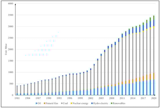
Figure 1.
Energy consumption from 1981 to 2020 in China.
To accurately reflect the actual situation in China, the variables were processed into per capita values. Table 1 gives the statistical summary of the data utilized in the analysis. In addition, Figure 2 and Figure 3 exhibit the trends of per capita values of the variables over years. Figure 2 illustrates that fossil fuel consumption, after a significant increase in 2002, gradually stabilized over time, whereas alternative energy consumption has shown exponential growth in recent years. Meanwhile, Figure 3 portrays the changing trend in CO2 emissions, which resembles the curve of fossil fuel consumption, while GDP continues to grow rapidly.

Table 1.
Descriptive statistics of variables.

Figure 2.
Trend of per capita fossil fuel and alternative energy consumption from 1981 to 2020 in China.
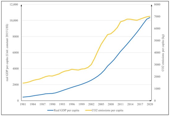
Figure 3.
Trend of per capita GDP and CO2 emissions from 1981 to 2020 in China.
4.2. Unit Root Analysis
The findings of the unit root test presented in Table 2 demonstrate that the variables selected are not stationary at their levels, and the null hypothesis of non-stationarity cannot be rejected. Additionally, the assessment of stationarity in the first difference, as indicated by the ADF and PP tests, shows that all the sequences are stationary in the first difference, and the null hypothesis of non-stationarity is rejected at the significance levels of 10%, 5%, and 1%. As all variables exhibit first-order integration, the use of ARDL bounds cointegration technique is considered appropriate.
Table 2.
Results of unit root tests.
4.3. ARDL Bounds Testing Results
After determining the order of integration of the variables, the ARDL bounds test is applied to assess the existence of long-term relationships between them. Given the sensitivity of the F test in ARDL to the lag length, the selection of the number of lags for each variable is critical. In this article, the appropriate lags were identified based on SBC, which, compared to AIC, selects the shortest lag length that minimizes the loss of degrees of freedom [47].
The results presented in Table 3 show that the F-statistics of each equation surpass the critical value upper limit, meaning that the null hypothesis of no cointegrating relationship is rejected at both 1% and 5% levels. Therefore, the bounds cointegration test provides evidence for the existence of a long-term relationship between per capita carbon dioxide emissions and per capita GDP, per capita fossil fuel consumption, and per capita alternative energy consumption.
Table 3.
Results of ARDL bounds tests.
4.4. The Long Run and Short Run Dynamics
Subsequently, after the existence of long-term relationships was confirmed, this study utilized the OLS method to estimate the long-term and short-term coefficients of the ARDL model, which are presented in Table 4.
Table 4.
Estimated coefficients from ARDL (1,0,1,2) model.
The long-term elasticity estimate β of per capita GDP is slightly less than zero but not statistically significant. The long-term estimated coefficient of per capita fossil fuel consumption indicates a highly significant impact on CO2 emissions in the long run. Specifically, an increase of 1% in fossil fuel consumption results in an increase of 1.0588% in CO2 emissions in the environment. This finding confirms the hypothesis H1, and it is consistent with previous studies [17,18,23,28,30]. The significant role of fossil fuels in promoting large CO2 emissions calls for policymakers to provide incentives for energy conservation and the use of environmentally friendly energy. The result of the coefficient of per capita alternative energy consumption is negative and statistically significant, meaning a 1% increase in alternative energy consumption would reduce CO2 emissions by 0.0523%. This finding, supporting the hypothesis H2 and similar to previous studies [13,31,35,36,37,38], demonstrates that the scale of alternative energy in China has already been able to significantly reduce CO2 emissions in the environment, which suggests the important role of substituting fossil fuels with environmentally friendly energy to reduce emissions.
The results of the short-term coefficient estimates presented in Table 4 show a positive but not statistically significant short-term elasticity of per capita GDP. The positive impact of per capita fossil fuel consumption on CO2 emissions remains significant and substantial in the short term. The short-term coefficient of per capita alternative energy consumption is slightly greater than zero and not statistically significant, which differs from its long-term performance. This may be due to the fact that the rapid development of alternative energy in China, such as nuclear power plants, dams, wind farms, and other infrastructure construction, has a significant promotion impact on CO2 emissions in the short term [39]. In other words, energy replacement is a long-term process, which is why alternative energy consumption has not achieved emissions reduction in the short term.
The computed coefficient for ECT is statistically significant at a 1% level and exhibits a negative value. This implies that the imbalanced per capita CO2 emissions resulting from the previous year’s shock was partially alleviated to the extent of 28.71% in the current year, bringing it closer to the long-term equilibrium state. To put it in perspective, it is estimated that full restoration of the long-term equilibrium would occur after approximately three and a half years.
In addition, this paper runs diagnostic procedures for the ARDL model, including Normality, Correlation LM, ARCH, and Ramsey RESET tests for the normality, correlation, heteroscedasticity, and functional form of the residuals, respectively. The diagnostic probabilities in Table 4 are greater than 0.05, indicating that the established ARDL model is stable.
The stability of the long-term and short-term coefficients is also tested through the CUSUM and CUSUMSQ of the recursive regression residuals provided by Brown et al. [65]. The CUSUM and CUSUMSQ statistical values depicted in Figure 4 and Figure 5 remain within the 5% significance bounds, indicating that all parameters derived from the regression are stable and the null hypothesis of stability cannot be rejected.

Figure 4.
The plot of the cumulative sum of recursive residuals (CUSUM). The dashed lines are critical boundaries at 5% significance level.
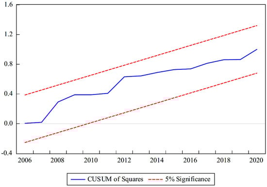
Figure 5.
The plot of the cumulative sum of squares of recursive residuals (CUSUMSQ). The dashed lines are critical boundaries at 5% significance level.
4.5. Johansen Maximum Likelihood Cointegration Tests
The results of the unit root test performed previously demonstrate that the data meets the requirements for using the Johansen cointegration test. The optimal lag section for the VAR framework, which considers per capita CO2 emissions, per capita GDP, per capita fossil fuel consumption, and per capita alternative energy consumption, is presented in Table 5. The results indicate that the best lag length for the multivariate VAR model is two.
Table 5.
Test statistics and choice criteria for selecting the order of the model.
The Johansen cointegration test analyzes the trace statistic and maximum eigenvalue statistic, which are presented in Table 6. The results indicate that at least one cointegration relationship exists between per capita carbon dioxide emissions, per capita GDP, per capita fossil fuel consumption, and per capita alternative energy consumption. The null hypothesis of no cointegrating relationship is rejected at a significance level of 5%. This implies that the findings of the ARDL bounds test are robust and valid.
Table 6.
Results of Johansen cointegration tests.
4.6. VECM Granger Causality Approach
The casual relationships between variables were explored through the use of a vector error correction-based Granger causality model, including both short-term and long-term Granger causality. The results of the Granger causality model are summarized in Table 7.
Table 7.
Results of VECM Granger causality analysis.
The results presented in Table 7 reveal the existence of a long-term unidirectional causal relationship from carbon emissions, fossil fuels, and alternative energy to GDP. In terms of short-term causal relationships, a unidirectional causal relationship from carbon emissions to GDP was observed. Additionally, evidence suggests that there is also a short-term unidirectional causal relationship from fossil fuels to GDP. Thus, there is a strong causal relationship from carbon emissions and fossil fuels to GDP, revealing that China’s economic growth is still dominated by fossil fuels that pollute the environment. China needs to adopt alternative energy as soon as possible to achieve its emission reduction target. Furthermore, a short-term unidirectional causal relationship from GDP to alternative energy was found, indicating that economic growth is beneficial for the advancement of alternative energy.
Additionally, the normality, autocorrelation, and heteroscedasticity of the residuals of the VECM model were diagnosed in this study. The diagnostic probabilities presented in the bottom of Table 7 are greater than 5%, indicating that the established VECM model is stable.
5. Conclusions and Policy Implications
This study aims to evaluate the impacts of fossil fuel consumption, alternative energy consumption, and economic growth on CO2 emissions in China between 1981 and 2020 within a multi-variable framework. The ARDL bounds testing approach, supplemented by the Johansen likelihood procedure, is utilized to explore the long-term cointegration relationship between endogenous and exogenous variables. Furthermore, the VECM Granger causality test is employed to analyze the causal connections between variables in both the long and short run. The results of the unit root test affirm the applicability of using these models for time series analysis. The stability of the model is established through the use of diagnostic tests, and the stability of the parameter estimates is confirmed through the application of CUSUM and CUSUMSQ.
The empirical results of this study highlight the following key discoveries:
Firstly, the findings from ARDL and Johansen cointegration test revealed that the coefficient of fossil fuel consumption had a positive and significant effect on CO2 emissions in both the long- and short-run in China. On the other hand, the coefficient of alternative energy consumption displayed a negative impact on CO2 emissions in the long-run, but no statistically significant influence in the short-run. These results indicated that the substitution of fossil fuels with environmentally friendly energy played a crucial role in achieving carbon reduction targets in the long-term. Furthermore, given the relatively small value of alternative energy’s coefficient in the cointegration equation, these empirical findings can be attributed to the limited scale of alternative energy in China. Therefore, to facilitate the transition towards a low-carbon economy, the expansion of the alternative energy sector should be prioritized.
Additionally, the findings from VECM Granger causality test demonstrated that there was a long-term unidirectional causal interaction from CO2 emissions, fossil fuel consumption, and alternative energy consumption to economic growth in China (co, fossil, alter→gdp). In the short run, unidirectional causal relationships, such as co→gdp, fossil→gdp and gdp→alter, were observed. Notably, this article found the unidirectional causal relationship fossil→gdp→alter, which suggested that fossil fuels, as an engine of economic growth, had an indirect effect on facilitating the development of alternative energy. The results indicated that reducing fossil fuel consumption drastically in the short-term may indirectly slow down the process of energy substitution.
The findings of the study informed us that the substitution of fossil fuels with alternative energy is a gradual and long-term process. Based on the results, our study has several important implications for China.
Firstly, the Chinese government should establish new environmental policies to control the expansion of fossil fuels. Specifically, enterprises should be targeted, and the government must enforce measures to enhance energy efficiency. Punitive actions may be taken against energy-inefficient enterprises to encourage them to improve their energy usage and gradually reduce their reliance on fossil fuels.
Secondly, the government should concentrate on expanding alternative energy and formulate proactive policies. For instance, the government can increase financial investment in alternative energy solutions and provide them to enterprises, thereby gradually transitioning to alternative energy in the long run. Furthermore, policymakers should promote the advancement of green technologies and scientific innovation. This could be achieved by enhancing research funding in educational institutions, especially in green technologies, to facilitate green innovation. In order to complement these policies, the government might also improve the educational curriculums for environmental sustainability and environmental issues [68] and increase awareness among enterprises and local communities about the benefits of alternative energy solutions.
Overall, this paper provides policies to curb fossil fuel growth and expand alternative energy, including the penalization of energy-inefficient enterprises, the encouragement of technological innovation, the promotion environmental education, and the adoption of alternative energy solutions. The research seeks to contribute to the development of evidence-based policies and support to achieve China’s carbon mitigation targets.
Despite the contribution to the current literature, this study has some limitations. For instance, this research is only restricted to the context of China. Future studies can be conducted on the provincial level to investigate energy substitution and carbon reduction strategies by using more updated data. In addition, alternative cointegration techniques, such as nonlinear autoregressive distributed lag (NARDL) model, could be employed in further studies. This method decomposes data into increasing and decreasing parts, evaluating the asymmetries of the responsiveness of socio-economic variables to their determinants [69,70], which will yield innovative policy instruments.
Author Contributions
Conceptualization, H.T., H.M. and N.L.; methodology, H.T. and P.W.; software, H.T.; formal analysis and data curation, H.T.; writing—original draft, H.T.; writing—review and editing, H.M., N.L. and P.W.; funding acquisition, H.M. All authors have read and agreed to the published version of the manuscript.
Funding
The authors gratefully acknowledge the financial support from the National Natural Science Foundation of China (51976020) and the National Natural Science Foundation of China (71603039).
Data Availability Statement
The data used in the current study are available in the World Development Indicators online database, the British Petroleum Statistical Review, and other public resources.
Acknowledgments
We would like to express our gratitude to Yuguang Dai from Dalian Thunder Software Technology Co., Ltd. for his contributions to the software aspect of the paper. Furthermore, we would like to thank the editor and anonymous referees for their constructive suggestions and valuable comments on the earlier draft of this paper, upon which we have improved the content.
Conflicts of Interest
The authors declare no conflict of interest.
References
- Azam, A.; Rafiq, M.; Shafique, M.; Zhang, H.; Yuan, J. Analyzing the effect of natural gas, nuclear energy and renewable energy on GDP and carbon emissions: A multi-variate panel data analysis. Energy 2021, 219, 119592. [Google Scholar] [CrossRef]
- Jin, T.; Kim, J. What is better for mitigating carbon emissions–Renewable energy or nuclear energy? A panel data analysis. Renew. Sustain. Energy Rev. 2018, 91, 464–471. [Google Scholar] [CrossRef]
- Dale, S. BP Statistical Review of World Energy; BP Plc.: London, UK, 2021; pp. 14–16. [Google Scholar]
- Liu, Z.; Deng, Z.; He, G.; Wang, H.; Zhang, X.; Lin, J.; Qi, Y.; Liang, X. Challenges and opportunities for carbon neutrality in China. Nat. Rev. Earth Environ. 2022, 3, 141–155. [Google Scholar] [CrossRef]
- Musa, S.D.; Zhonghua, T.; Ibrahim, A.O.; Habib, M. China’s energy status: A critical look at fossils and renewable options. Renew. Sustain. Energy Rev. 2018, 81, 2281–2290. [Google Scholar] [CrossRef]
- Zhang, S.; Chen, W. Assessing the energy transition in China towards carbon neutrality with a probabilistic framework. Nat. Commun. 2022, 13, 87. [Google Scholar] [CrossRef]
- Yu, S.; Yarlagadda, B.; Siegel, J.E.; Zhou, S.; Kim, S. The role of nuclear in China’s energy future: Insights from integrated assessment. Energy Policy 2020, 139, 111344. [Google Scholar] [CrossRef]
- Song, D.; Liu, Y.; Qin, T.; Gu, H.; Cao, Y.; Shi, H. Overview of the policy instruments for renewable energy development in China. Energies 2022, 15, 6513. [Google Scholar] [CrossRef]
- IEA. World Energy Outlook; IEA: Paris, France, 2021. [Google Scholar]
- Antonakakis, N.; Chatziantoniou, I.; Filis, G. Energy consumption, CO2 emissions, and economic growth: An ethical dilemma. Renew. Sustain. Energy Rev. 2017, 68, 808–824. [Google Scholar] [CrossRef]
- Acaravci, A.; Ozturk, I. On the relationship between energy consumption, CO2 emissions and economic growth in Europe. Energy 2010, 35, 5412–5420. [Google Scholar] [CrossRef]
- Jin, T. The evolutionary renewable energy and mitigation impact in OECD countries. Renew. Energy 2022, 189, 570–586. [Google Scholar] [CrossRef]
- Dogan, E.; Seker, F. The influence of real output, renewable and non-renewable energy, trade and financial development on carbon emissions in the top renewable energy countries. Renew. Sustain. Energy Rev. 2016, 60, 1074–1085. [Google Scholar] [CrossRef]
- Sebri, M.; Ben-Salha, O. On the causal dynamics between economic growth, renewable energy consumption, CO2 emissions and trade openness: Fresh evidence from BRICS countries. Renew. Sustain. Energy Rev. 2014, 39, 14–23. [Google Scholar] [CrossRef]
- Bildirici, M.E.; Gökmenoğlu, S.M. Environmental pollution, hydropower energy consumption and economic growth: Evidence from G7 countries. Renew. Sustain. Energy Rev. 2017, 75, 68–85. [Google Scholar] [CrossRef]
- Salim, R.A.; Rafiq, S. Why do some emerging economies proactively accelerate the adoption of renewable energy? Energy Econ. 2012, 34, 1051–1057. [Google Scholar] [CrossRef]
- Amri, F. Carbon dioxide emissions, output, and energy consumption categories in Algeria. Environ. Sci. Pollut. Res. 2017, 24, 14567–14578. [Google Scholar] [CrossRef] [PubMed]
- Yuping, L.; Ramzan, M.; Xincheng, L.; Murshed, M.; Awosusi, A.A.; BAH, S.I.; Adebayo, T.S. Determinants of carbon emissions in Argentina: The roles of renewable energy consumption and globalization. Energy Rep. 2021, 7, 4747–4760. [Google Scholar] [CrossRef]
- Long, X.; Naminse, E.Y.; Du, J.; Zhuang, J. Nonrenewable energy, renewable energy, carbon dioxide emissions and economic growth in China from 1952 to 2012. Renew. Sustain. Energy Rev. 2015, 52, 680–688. [Google Scholar] [CrossRef]
- Jayanthakumaran, K.; Verma, R.; Liu, Y. CO2 emissions, energy consumption, trade and income: A comparative analysis of China and India. Energy Policy 2012, 42, 450–460. [Google Scholar] [CrossRef]
- Ghosh, S. Examining carbon emissions economic growth nexus for India: A multivariate cointegration approach. Energy Policy 2010, 38, 3008–3014. [Google Scholar] [CrossRef]
- Shahbaz, M.; Hye, Q.M.A.; Tiwari, A.K.; Leitão, N.C. Economic growth, energy consumption, financial development, international trade and CO2 emissions in Indonesia. Renew. Sustain. Energy Rev. 2013, 25, 109–121. [Google Scholar] [CrossRef]
- Salahuddin, M.; Alam, K.; Ozturk, I.; Sohag, K. The effects of electricity consumption, economic growth, financial development and foreign direct investment on CO2 emissions in Kuwait. Renew. Sustain. Energy Rev. 2018, 81, 2002–2010. [Google Scholar] [CrossRef]
- Ali, W.; Abdullah, A.; Azam, M. Re-visiting the environmental Kuznets curve hypothesis for Malaysia: Fresh evidence from ARDL bounds testing approach. Renew. Sustain. Energy Rev. 2017, 77, 990–1000. [Google Scholar] [CrossRef]
- Rafindadi, A.A. Does the need for economic growth influence energy consumption and CO2 emissions in Nigeria? Evidence from the innovation accounting test. Renew. Sustain. Energy Rev. 2016, 62, 1209–1225. [Google Scholar] [CrossRef]
- Hussain, I.; Rehman, A. Exploring the dynamic interaction of CO2 emission on population growth, foreign investment, and renewable energy by employing ARDL bounds testing approach. Environ. Sci. Pollut. Res. 2021, 28, 39387–39397. [Google Scholar] [CrossRef]
- Zambrano-Monserrate, M.A.; Silva-Zambrano, C.A.; Davalos-Penafiel, J.L.; Zambrano-Monserrate, A.; Ruano, M.A. Testing environmental Kuznets curve hypothesis in Peru: The role of renewable electricity, petroleum and dry natural gas. Renew. Sustain. Energy Rev. 2018, 82, 4170–4178. [Google Scholar] [CrossRef]
- Mezghani, I.; Haddad, H.B. Energy consumption and economic growth: An empirical study of the electricity consumption in Saudi Arabia. Renew. Sustain. Energy Rev. 2017, 75, 145–156. [Google Scholar] [CrossRef]
- Talbi, B. CO2 emissions reduction in road transport sector in Tunisia. Renew. Sustain. Energy Rev. 2017, 69, 232–238. [Google Scholar] [CrossRef]
- Bulut, U. The impacts of non-renewable and renewable energy on CO2 emissions in Turkey. Environ. Sci. Pollut. Res. 2017, 24, 15416–15426. [Google Scholar] [CrossRef]
- Dogan, E.; Ozturk, I. The influence of renewable and non-renewable energy consumption and real income on CO2 emissions in the USA: Evidence from structural break tests. Environ. Sci. Pollut. Res. 2017, 24, 10846–10854. [Google Scholar] [CrossRef]
- Jalil, A.; Feridun, M. The impact of growth, energy and financial development on the environment in China: A cointegration analysis. Energy Econ. 2011, 33, 284–291. [Google Scholar] [CrossRef]
- Alshehry, A.S.; Belloumi, M. Study of the environmental Kuznets curve for transport carbon dioxide emissions in Saudi Arabia. Renew. Sustain. Energy Rev. 2017, 75, 1339–1347. [Google Scholar] [CrossRef]
- Wang, B.; Wang, Z. Imported technology and CO2 emission in China: Collecting evidence through bound testing and VECM approach. Renew. Sustain. Energy Rev. 2018, 82, 4204–4214. [Google Scholar]
- Iwata, H.; Okada, K.; Samreth, S. Empirical study on the environmental Kuznets curve for CO2 in France: The role of nuclear energy. Energy Policy 2010, 38, 4057–4063. [Google Scholar] [CrossRef]
- Bölük, G.; Mert, M. The renewable energy, growth and environmental Kuznets curve in Turkey: An ARDL approach. Renew. Sustain. Energy Rev. 2015, 52, 587–595. [Google Scholar] [CrossRef]
- Solarin, S.A.; Al-Mulali, U.; Ozturk, I. Validating the environmental Kuznets curve hypothesis in India and China: The role of hydroelectricity consumption. Renew. Sustain. Energy Rev. 2017, 80, 1578–1587. [Google Scholar] [CrossRef]
- Onater-Isberk, E. Environmental Kuznets curve under noncarbohydrate energy. Renew. Sustain. Energy Rev. 2016, 64, 338–347. [Google Scholar] [CrossRef]
- Lin, B.; Moubarak, M. Renewable energy consumption–economic growth nexus for China. Renew. Sustain. Energy Rev. 2014, 40, 111–117. [Google Scholar] [CrossRef]
- Bhattacharya, M.; Paramati, S.R.; Ozturk, I.; Bhattacharya, S. The effect of renewable energy consumption on economic growth: Evidence from top 38 countries. Appl. Energy 2016, 162, 733–741. [Google Scholar] [CrossRef]
- Dong, F.; Li, Y.; Gao, Y.; Zhu, J.; Qin, C.; Zhang, X. Energy transition and carbon neutrality: Exploring the non-linear impact of renewable energy development on carbon emission efficiency in developed countries. Resour. Conserv. Recycl. 2022, 177, 106002. [Google Scholar] [CrossRef]
- Ohlan, R. The impact of population density, energy consumption, economic growth and trade openness on CO2 emissions in India. Nat. Hazards 2015, 79, 1409–1428. [Google Scholar] [CrossRef]
- Lin, B.; Omoju, O.E.; Okonkwo, J.U. Impact of industrialisation on CO2 emissions in Nigeria. Renew. Sustain. Energy Rev. 2015, 52, 1228–1239. [Google Scholar] [CrossRef]
- Ali, W.; Abdullah, A.; Azam, M. The dynamic relationship between structural change and CO2 emissions in Malaysia: A cointegrating approach. Environ. Sci. Pollut. Res. 2017, 24, 12723–12739. [Google Scholar] [CrossRef] [PubMed]
- List, J.A.; Gallet, C.A. The environmental Kuznets curve: Does one size fit all? Ecol. Econ. 1999, 31, 409–423. [Google Scholar] [CrossRef]
- Saboori, B.; Sulaiman, J.; Mohd, S. Economic growth and CO2 emissions in Malaysia: A cointegration analysis of the environmental Kuznets curve. Energy Policy 2012, 51, 184–191. [Google Scholar] [CrossRef]
- Jalil, A.; Mahmud, S.F. Environment Kuznets curve for CO2 emissions: A cointegration analysis for China. Energy Policy 2009, 37, 5167–5172. [Google Scholar] [CrossRef]
- Zhao, C.; Chen, B.; Hayat, T.; Alsaedi, A.; Ahmad, B. Driving force analysis of water footprint change based on extended STIRPAT model: Evidence from the Chinese agricultural sector. Ecol. Indic. 2014, 47, 43–49. [Google Scholar] [CrossRef]
- Gingrich, S.; Kušková, P.; Steinberger, J.K. Long-term changes in CO2 emissions in Austria and Czechoslovakia—Identifying the drivers of environmental pressures. Energy Policy 2011, 39, 535–543. [Google Scholar] [CrossRef]
- Engle, R.F.; Granger, C.W. Co-integration and error correction: Representation, estimation, and testing. Econom. J. Econom. Soc. 1987, 55, 251–276. [Google Scholar] [CrossRef]
- Johansen, S. Statistical analysis of cointegration vectors. J. Econ. Dyn. Control 1988, 12, 231–254. [Google Scholar] [CrossRef]
- Pesaran, M.H.; Shin, Y. An Autoregressive Distributed Lag Modelling Approach to Cointegration Analysis; Cambridge University Press: Cambridge, UK, 1995. [Google Scholar]
- Pesaran, M.H.; Shin, Y.; Smith, R.P. Pooled mean group estimation of dynamic heterogeneous panels. J. Am. Stat. Assoc. 1999, 94, 621–634. [Google Scholar] [CrossRef]
- Pesaran, M.H.; Shin, Y.; Smith, R.J. Bounds testing approaches to the analysis of level relationships. J. Appl. Econom. 2001, 16, 289–326. [Google Scholar] [CrossRef]
- Johansen, S.; Juselius, K. Maximum likelihood estimation and inference on cointegration—With appucations to the demand for money. Oxf. Bull. Econ. Stat. 1990, 52, 169–210. [Google Scholar] [CrossRef]
- Phillips, P.C.; Hansen, B.E. Statistical inference in instrumental variables regression with I (1) processes. Rev. Econ. Stud. 1990, 57, 99–125. [Google Scholar] [CrossRef]
- Narayan, P.K. The saving and investment nexus for China: Evidence from cointegration tests. Appl. Econ. 2005, 37, 1979–1990. [Google Scholar] [CrossRef]
- Dickey, D.A.; Fuller, W.A. Distribution of the estimators for autoregressive time series with a unit root. J. Am. Stat. Assoc. 1979, 74, 427–431. [Google Scholar]
- Phillips, P.C.; Perron, P. Testing for a unit root in time series regression. Biometrika 1988, 75, 335–346. [Google Scholar] [CrossRef]
- Jarque, C.M.; Bera, A.K. A test for normality of observations and regression residuals. Int. Stat. Rev./Rev. Int. Stat. 1987, 55, 163–172. [Google Scholar] [CrossRef]
- Breusch, T.S. Testing for autocorrelation in dynamic linear models. Aust. Econ. Pap. 1978, 17, 334–355. [Google Scholar] [CrossRef]
- Godfrey, L.G. Testing against general autoregressive and moving average error models when the regressors include lagged dependent variables. Econom. J. Econom. Soc. 1978, 46, 1293–1301. [Google Scholar] [CrossRef]
- Bollerslev, T. Generalized autoregressive conditional heteroskedasticity. J. Econom. 1986, 31, 307–327. [Google Scholar] [CrossRef]
- Ramsey, J.B. Tests for specification errors in classical linear least-squares regression analysis. J. R. Stat. Soc. Ser. B (Methodol.) 1969, 31, 350–371. [Google Scholar] [CrossRef]
- Brown, R.L.; Durbin, J.; Evans, J.M. Techniques for testing the constancy of regression relationships over time. J. R. Stat. Soc. Ser. B (Methodol.) 1975, 37, 149–163. [Google Scholar] [CrossRef]
- Sims, C.A. Macroeconomics and reality. Econom. J. Econom. Soc. 1980, 48, 1–48. [Google Scholar] [CrossRef]
- Granger, C.W. Investigating causal relations by econometric models and cross-spectral methods. Econom. J. Econom. Soc. 1969, 37, 424–438. [Google Scholar] [CrossRef]
- Spreafico, C.; Landi, D. Investigating students’ eco-misperceptions in applying eco-design methods. J. Clean. Prod. 2022, 342, 130866. [Google Scholar] [CrossRef]
- Sadik-Zada, E.R.; Niklas, B. Business cycles and alcohol consumption: Evidence from a nonlinear panel ARDL approach. J. Wine Econ. 2021, 16, 429–438. [Google Scholar] [CrossRef]
- Niklas, B.; Sadik-Zada, E.R. Income inequality and status symbols: The case of fine wine imports. J. Wine Econ. 2019, 14, 365–373. [Google Scholar] [CrossRef]
Disclaimer/Publisher’s Note: The statements, opinions and data contained in all publications are solely those of the individual author(s) and contributor(s) and not of MDPI and/or the editor(s). MDPI and/or the editor(s) disclaim responsibility for any injury to people or property resulting from any ideas, methods, instructions or products referred to in the content. |
© 2023 by the authors. Licensee MDPI, Basel, Switzerland. This article is an open access article distributed under the terms and conditions of the Creative Commons Attribution (CC BY) license (https://creativecommons.org/licenses/by/4.0/).