Fault Detection of Induction Motors with Combined Modeling- and Machine-Learning-Based Framework

Abstract

This paper deals with the early detection of fault conditions in induction motors using a combined model- and machine-learning-based approach with flexible adaptation to individual motors. The method is based on analytical modeling in the form of a multiple coupled circuit model and a feedforward neural network. In addition, the differential evolution algorithm independently identifies the parameters of the motor for the multiple coupled circuit model based on easily obtained measurement data from a healthy state. With the identified parameters, the multiple coupled circuit model is used to perform dynamic simulations of the various fault cases of the specific induction motor. The simulation data set of the stator currents is used to train the neural network for classification of different stator, rotor, mechanical, and voltage supply faults. Finally, the combined method is successfully validated with measured data of faults in an induction motor, proving the transferability of the simulation-trained neural network to a real environment. Neglecting bearing faults, the fault cases from the validation data are classified with an accuracy of 94.81%.

1. Introduction

Squirrel cage induction motors are often an essential part of industrial processes and are widely used in various industries due to their robust characteristics. Failures and repairs of individual machines or complete systems can quickly lead to high costs in the industrial environment, as well as a large demand for additional manpower and time. Continuous monitoring and early detection of electrical drive fault conditions offer a potential solution to such problems. These tools can help ensure reliable and predictable machine operation. For the above reasons, the early detection and diagnosis of fault conditions in induction motors and other types of electric drives have been a highly regarded research topic, as evidenced by various review publications [1,2,3]. According to Gao et al., fault diagnosis methods are generally classified into model-based, signal-based, and data-based approaches [4]: Model-based methods use models for fault diagnosis by monitoring the correlation between the real systems and the models. Signal-based methods utilize measured signals that reflect the fault cases. A diagnostic decision is made based on the extracted features and previous experience about the features in the healthy and faulty states. Data-based approaches use only existing data sets for fault detection. No prior knowledge is required.

Traditionally, signal-based approaches have played a major role in induction machine fault detection [5]. A classic method is the motor current signature analysis (MCSA), whose main objective is a high-resolution Fourier analysis of the stator currents in order to identify specific frequency components [6,7]. The stator currents are also considered in approaches using the Park vector, which transforms the three-phase current into a two-dimensional representation. When a fault condition occurs, the shape of the representation changes compared to the healthy state, allowing the fault condition to be detected [8,9]. In addition, more sophisticated signal-based methods exist, such as the discrete wavelet transform (DWT), which has the advantage of providing powerful frequency analysis of non-stationary signals [10,11,12]. Similar methods are the Wigner–Ville distribution (WVD) [13] or the Hilbert–Huang transform (HHT) [14]. These methods allow analysis in the combined time and frequency domain and the detection of specific fault characteristics in this domain. As in most of the approaches described so far, stator currents are primarily used as the signals to be evaluated [15]. Alternatively, vibration measurements are also used [16,17], with each quantity having its own advantages and disadvantages [18]. Other approaches use an additional sensor to measure the magnetic flux [19,20,21] or a thermography camera [22,23] for fault detection, but like the vibration sensor, this involves additional effort and cost. Current sensors, on the other hand, are usually present in all motors. In general, the signal-based approaches can be applied to all fault cases, such as short circuits in the stator [24,25], broken cage bars or end rings [26,27], eccentricities [17,28], or bearing faults [29,30]. The disadvantages of these signal-based methods are that they require precise prior knowledge of the specific fault characteristics, and the detection must often be manually adapted to the particular motor.

Due to major advances in the field of artificial intelligence (AI) and machine learning (ML), data-based approaches for induction machine fault diagnosis have been increasingly developed [31,32]. The advantage over signal-based methods is that now no specific prior knowledge of the fault characteristics and no manual analysis of the signals is required [33]. All that is required is the acquisition of a sufficient amount of data, and the corresponding algorithms learn the necessary fault characteristics independently. In the field of machine learning, there are different methods available, such as the support vector machine (SVM) [34,35,36], the k-nearest neighbors (kNN) algorithm [35,36], and different types of neural networks, such as regular feedforward neural networks (FFNN) [37,38,39], convolutional neural networks (CNN) [40,41], recurrent neural networks (RNN) [42,43], autoencoders (AE) [44,45], or deep belief networks (DBN) [45]. The publications listed so far deal with several fault cases, but individual approaches also focus on specific fault types, such as stator short circuits [46,47], broken rotor bars [48,49,50], or bearing faults [45,51,52]. A combination of signal-based and data-based methods is also common, with the signal-based approaches preprocessing the data to extract known fault features that the algorithms use for diagnosis [14,22,38,48]. However, the disadvantage of data-based methods is that enough data about the different healthy and faulty states must be available. In an industrial environment, detailed data acquisition for motors, especially for fault conditions, is problematic, making practical use impossible without a great deal of effort. Another possibility is to combine a model-based method with data-based methods. Such an approach is used by Murphey [53] and Masrur [54] to first generate data through modeling, which is then used to train an AI and classify faults in the voltage supply. The basic idea of such a method is advantageous because there is no need for expensive measurements of the motor in the different fault cases. Instead, appropriate modeling is used to generate data on the behavior of the motor in the healthy and fault states. However, a crucial step is missing to ensure practicability. This is because the parameters of the motor are also required to reproduce its behavior. Determining these parameters, whether by different test methods [55,56] or finite element analysis [57], is very time-consuming and thus hinders practical implementation.

In the approach presented here, a method for fault detection of squirrel cage induction motors is demonstrated, which identifies the parameters for modeling in advance from easily measurable quantities. The modeling is based on a multiple coupled circuit model whose parameters are identified using the differential evolution (DE) algorithm by comparing the simulation results with real measured data. Finally, the data set generated by the model is used to train a feedforward neural network for fault detection. The contribution of this paper aims at the practicable application of fault detection in the industry. By combining modeling and machine learning, the monitoring of an induction motor can be conducted with little prior knowledge, low effort, and already existing measurement technology. The structure of this paper leads through the different aspects of the method. In Section 2, the theoretical background of the modeling, the differential evolution algorithm, and neural networks are presented. Then, in Section 3, the interaction of the individual components within the overall framework is described. Section 4 shows the experimental setup in detail, leading to the validation and results in Section 5 and the conclusions in Section 6.

2. Theoretical Background

First, the technical background of the main aspects used in the approach is presented. This includes the modeling of the induction motor with squirrel cage rotor based on the multiple coupled circuit model together with the modified winding function method, which is used to calculate the self and mutual inductances. In addition to the healthy state modeling, the effects of the fault cases on the modeling are described. In addition, the mathematical background of the differential evolution algorithm and neural networks is briefly explained.

2.1. Induction Machine Modeling

A variety of model approaches exist for calculating the behavior of squirrel cage induction motors. Models based on a transformation into an arbitrary reference frame [58] do not allow the precise calculation of faults such as winding short circuits and are therefore not suited for fault detection. The finite element method (FEM), on the other hand, can be used to perform very complex simulations [59,60]. However, this approach is also not optimal for practical fault detection because of the high computational and time requirements. For comprehensive and flexible fault detection, the multiple coupled circuit model [61] is well-suited. This analytical modeling approach is based on the electrical network of the machine. With this type of modeling, the static and dynamic behavior as well as several fault types can be calculated [62]. The inductances for the modeling are usually estimated with the winding function method (WFM). This approach utilizes the distribution of the respective windings and geometrical quantities of the machine [63]. The modified winding function method (MWFM) is an extension of the original approach. Unlike the basic version, it is possible to calculate the inductances with variable air gap thicknesses [64].

2.1.1. Modeling Basic Machine

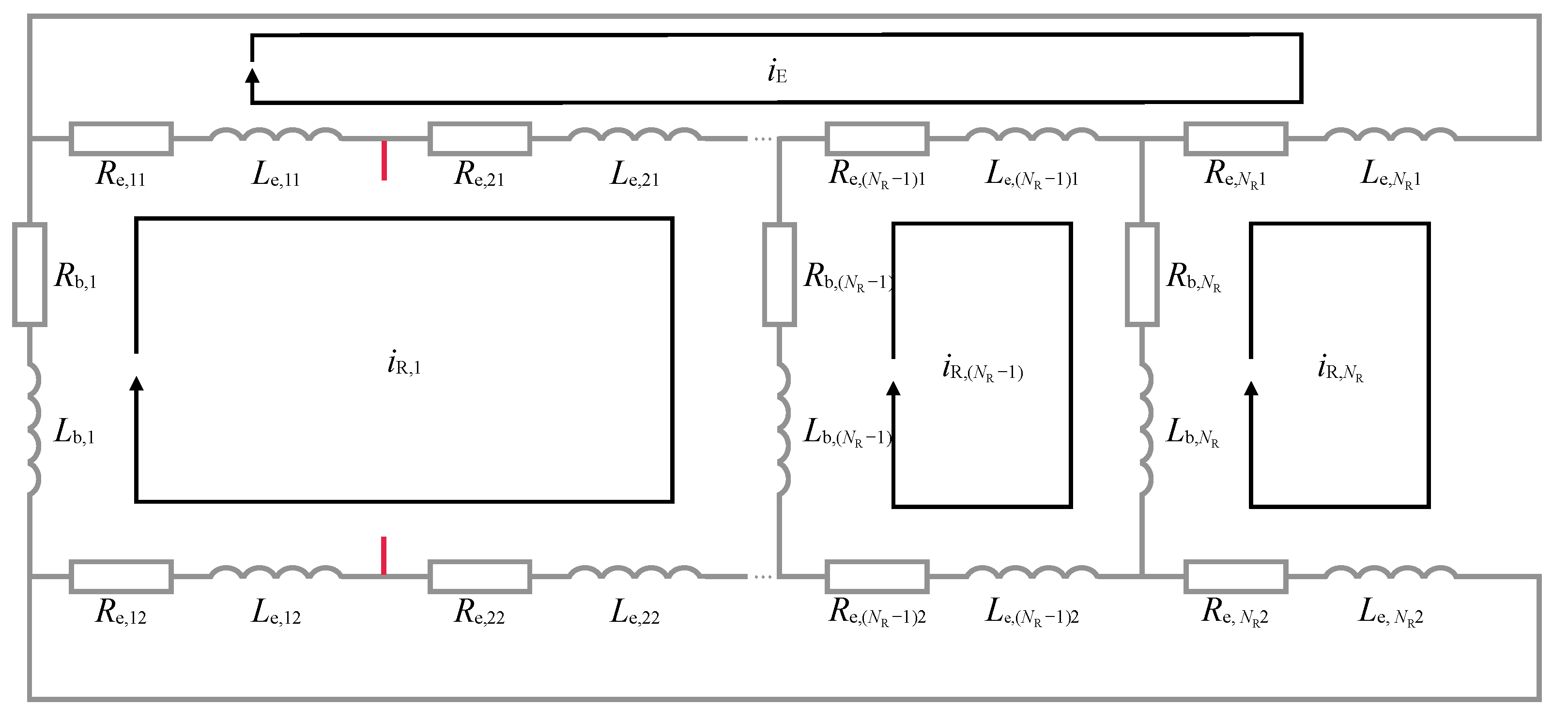
The theory of the modeling in this chapter originates from Toliyat et al. [61]. The central component of the model is the voltage equation with the corresponding resistances R, leakage inductances L, and inductances M. The voltages and currents of the three stator phases $U_{\mathrm{S}}$ and $i_{\mathrm{S}}$ and the rotor loops $U_{\mathrm{R}}$ and $i_{\mathrm{R}}$ are considered individually. Due to $N_{\mathrm{R}}$ cage bars in the rotor, $N_{\mathrm{R}}$ loop currents and an end ring current $i_{\mathrm{E}}$ exist for the rotor currents $i_{\mathrm{R}}$ (see Figure 1). The squirrel cage rotor causes zero values for the rotor voltages $U_{\mathrm{R}}$ [61]:

$$\begin{array}{cc}\hfill \left[\begin{array}{c}\left[U_{\mathrm{S}}\right]\\ [U_{\mathrm{R}}]\end{array}\right]& =\left[\begin{array}{cc}\left[R_{\mathrm{S}}\right]& 0\\ 0& \left[R_{\mathrm{R}}\right]\end{array}\right]\left[\begin{array}{c}\left[i_{\mathrm{S}}\right]\\ [i_{\mathrm{R}}]\end{array}\right]+\left[\begin{array}{cc}\left[L_{\mathrm{S}}\right]& 0\\ 0& \left[L_{\mathrm{R}}\right]\end{array}\right]\frac{\mathrm{d}}{\mathrm{d}t}\left[\begin{array}{c}\left[i_{\mathrm{S}}\right]\\ [i_{\mathrm{R}}]\end{array}\right]\hfill \\ & +\frac{\mathrm{d}}{\mathrm{d}t}\left(\left[\begin{array}{cc}\left[M_{\mathrm{SS}}\right]& \left[M_{\mathrm{SR}}\right]\\ [M_{\mathrm{RS}}]& \left[M_{\mathrm{RR}}\right]\end{array}\right]\left[\begin{array}{c}\left[i_{\mathrm{S}}\right]\\ [i_{\mathrm{R}}]\end{array}\right]\right)\hfill \end{array}$$

(1)

$$\left[\begin{array}{c}{U}_{\mathrm{S}}\end{array}\right]=\left[\begin{array}{c}{U}_{\mathrm{S},\mathrm{a}}\\ U_{\mathrm{S},\mathrm{b}}\\ U_{\mathrm{S},\mathrm{c}}\end{array}\right]\left[\begin{array}{c}{i}_{\mathrm{S}}\end{array}\right]=\left[\begin{array}{c}{i}_{\mathrm{S},\mathrm{a}}\\ i_{\mathrm{S},\mathrm{b}}\\ i_{\mathrm{S},\mathrm{c}}\end{array}\right]\left[\begin{array}{c}{U}_{\mathrm{R}}\end{array}\right]=0\left[\begin{array}{c}{i}_{\mathrm{R}}\end{array}\right]=\left[\begin{array}{c}{i}_{\mathrm{R},1}\\ i_{\mathrm{R},2}\\ i_{\mathrm{R},3}\\ \cdots \\ i_{\mathrm{R},{\mathrm{N}}_{\mathrm{R}}}\\ i_{\mathrm{E}}\end{array}\right]$$

(2)

The individual windings of the stator phases are summarized for the stator resistance $R_{\mathrm{S}}$ and leakage inductance $L_{\mathrm{S}}$. The resistances $R_{\mathrm{b}}$ and leakage inductances $L_{\mathrm{b}}$ of the cage bars and the resistances $R_{\mathrm{e}}$ and leakage inductances $L_{\mathrm{e}}$ of the end ring segments build the matrices for the resistance $R_{\mathrm{R}}$ and leakage inductance $L_{\mathrm{R}}$ of the rotor (see Figure 1). The leakage inductance matrices L behave analogously to the resistance R and are therefore not shown separately below [61]:

$$\left[\begin{array}{c}{R}_{\mathrm{S}}\end{array}\right]=\left[\begin{array}{ccc}{R}_{\mathrm{S}}& 0& 0\\ 0& R_{\mathrm{S}}& 0\\ 0& 0& R_{\mathrm{S}}\end{array}\right]$$

(3)

$$\left[\begin{array}{c}{R}_{\mathrm{R}}\end{array}\right]=\left[\begin{array}{cccccc}2(R_{\mathrm{b}}+R_{\mathrm{e}})& -R_{\mathrm{b}}& 0& \cdots & -R_{\mathrm{b}}& -R_{\mathrm{e}}\\ -R_{\mathrm{b}}& 2(R_{\mathrm{b}}+R_{\mathrm{e}})& -R_{\mathrm{b}}& \cdots & 0& -R_{\mathrm{e}}\\ 0& -R_{\mathrm{b}}& 2(R_{\mathrm{b}}+R_{\mathrm{e}})& \cdots & 0& -R_{\mathrm{e}}\\ \cdots & \cdots & \cdots & \cdots & \cdots & \cdots \\ -R_{\mathrm{b}}& 0& 0& \cdots & 2(R_{\mathrm{b}}+R_{\mathrm{e}})& -R_{\mathrm{e}}\\ -R_{\mathrm{e}}& -R_{\mathrm{e}}& -R_{\mathrm{e}}& \cdots & -R_{\mathrm{e}}& N_{\mathrm{R}}·R_{\mathrm{e}}\end{array}\right]$$

(4)

For the self inductance of stator and rotor, the square matrices $M_{\mathrm{SS}}$ and $M_{\mathrm{RR}}$ are present. In these matrices the couplings of the stator phases to each other and rotor loops to each other are described. The only difference in the self inductance of the rotor $M_{\mathrm{RR}}$ is that no magnetic coupling with the end ring exists. The coupling between stator and rotor results in the mutual inductances $M_{\mathrm{SR}}$ and $M_{\mathrm{RS}}$, which specify the relationship between the stator phases and rotor loops. These two matrices are mirror symmetric [61]:

$$\left[\begin{array}{c}{M}_{\mathrm{SS}}\end{array}\right]=\left[\begin{array}{ccc}{M}_{\mathrm{Sa},\mathrm{Sa}}& M_{\mathrm{Sa},\mathrm{Sb}}& M_{\mathrm{Sa},\mathrm{Sc}}\\ M_{\mathrm{Sb},\mathrm{Sa}}& M_{\mathrm{Sb},\mathrm{Sb}}& M_{\mathrm{Sb},\mathrm{Sc}}\\ M_{\mathrm{Sc},\mathrm{Sa}}& M_{\mathrm{Sc},\mathrm{Sb}}& M_{\mathrm{Sc},\mathrm{Sc}}\end{array}\right]$$

(5)

$$\left[\begin{array}{c}{M}_{\mathrm{RR}}\end{array}\right]=\left[\begin{array}{ccccc}{M}_{\mathrm{R}1,\mathrm{R}1}& M_{\mathrm{R}1,\mathrm{R}2}& \cdots & M_{\mathrm{R}1,{\mathrm{RN}}_{\mathrm{R}}}& 0\\ M_{\mathrm{R}2,\mathrm{R}1}& M_{\mathrm{R}2,\mathrm{R}2}& \cdots & M_{\mathrm{R}2,{\mathrm{RN}}_{\mathrm{R}}}& 0\\ \cdots & \cdots & \cdots & \cdots & \cdots \\ M_{{\mathrm{RN}}_{\mathrm{R}},\mathrm{R}1}& M_{{\mathrm{RN}}_{\mathrm{R}},\mathrm{R}2}& \cdots & M_{{\mathrm{RN}}_{\mathrm{R}},{\mathrm{RN}}_{\mathrm{R}}}& 0\\ 0& 0& \cdots & 0& 0\end{array}\right]$$

(6)

$$\left[\begin{array}{c}{M}_{\mathrm{SR}}\end{array}\right]=\left[\begin{array}{ccccc}{M}_{\mathrm{Sa},\mathrm{R}1}& M_{\mathrm{Sa},\mathrm{R}2}& \cdots & M_{\mathrm{Sa},{\mathrm{RN}}_{\mathrm{R}}}& 0\\ M_{\mathrm{Sb},\mathrm{R}1}& M_{\mathrm{Sb},\mathrm{R}2}& \cdots & M_{\mathrm{Sb},{\mathrm{RN}}_{\mathrm{R}}}& 0\\ M_{\mathrm{Sc},\mathrm{R}1}& M_{\mathrm{Sc},\mathrm{R}2}& \cdots & M_{\mathrm{Sc},{\mathrm{RN}}_{\mathrm{R}}}& 0\end{array}\right]$$

(7)

$$\left[\begin{array}{c}{M}_{\mathrm{RS}}\end{array}\right]={\left[\begin{array}{c}{M}_{\mathrm{SR}}\end{array}\right]}^{\mathrm{T}}$$

(8)

In addition to the electrical description, the mechanical equation of motion is also important. Only in combination with the mechanical equation is it possible to calculate the rotor speed $\omega$ and the dynamic properties of the electrical machine. For this purpose, the moment of inertia J as well as the torque of the load machine $T_{\mathrm{L}}$ and the electrical machine $T_{\mathrm{el}}$ are required. The generated torque $T_{\mathrm{el}}$ results from the local derivation of the currents i and the inductances M [61]:

$$\frac{\mathrm{d}}{\mathrm{d}t}\omega =\frac{1}{J}(T_{\mathrm{el}}+T_{\mathrm{L}})$$

(9)

$$T_{\mathrm{el}}=\frac{1}{2}\left[\begin{array}{cc}{\left[i_{\mathrm{S}}\right]}^T& {\left[i_{\mathrm{R}}\right]}^T\end{array}\right]\frac{\partial }{\partial \phi }\left[\begin{array}{cc}\left[M_{\mathrm{SS}}\right]& \left[M_{\mathrm{SR}}\right]\\ [M_{\mathrm{RS}}]& \left[M_{\mathrm{RR}}\right]\end{array}\right]\left[\begin{array}{c}\left[i_{\mathrm{S}}\right]\\ [i_{\mathrm{R}}]\end{array}\right]$$

(10)

2.1.2. Inductance Calculation

The winding function method is used to calculate the self and mutual inductances M. This analytical method assumes an infinite permeability of iron and does not need any symmetry for the winding slots. Consequently, the coupling inductance $M_{\mathrm{A},\mathrm{B}}$ between any two windings A and B in an electrical machine can be calculated according to the following equation [63]:

$$M_{\mathrm{A},\mathrm{B}}\left(\phi \right)={\mu }_{0}rl{\int }_0^{2\pi }{n}_{\mathrm{A}}(\phi ,\theta )·N_{\mathrm{B}}(\phi ,\theta )·g^{-1}(\phi ,\theta )\mathrm{d}\theta$$

(11)

This equation contains the turn function $n_{\mathrm{A}}(\phi ,\theta )$, which describes the local distribution of the windings of A over the circumference $\theta$. In addition, the winding function $N_{\mathrm{B}}(\phi ,\theta )$ appears, which reflects the magnetomotive force of the windings of B. Other parameters used in the calculation are the machine length l, the stator core radius r, the air gap thickness g, and the vacuum permeability ${\mu }_0$. Thus, the equation allows determining the inductances $M\left(\phi \right)$ for the magnetic coupling between the individual stator phases and rotor loops as a function of the rotation angle $\phi$.

In the presence of a variable air gap, as in the case of an eccentric rotor, the equation must be extended to the modified winding function method because the average of the winding function is no longer zero. Al-Nuaim and Toliyat [64] describe the necessary steps to account for a variable air gap in detail. Finally, only the calculation of the winding function changes, where $\overline{N_{\mathrm{B}}}(\phi ,\theta )$ describes the average value of the winding function [64]:

$$N_{\mathrm{B}}(\phi ,\theta )=n_{\mathrm{B}}(\phi ,\theta )-\overline{N_{\mathrm{B}}}(\phi ,\theta )$$

(12)

$$\overline{N_{\mathrm{B}}}(\phi ,\theta )=\frac{1}{2\pi ·{\overline{g}}^{-1}(\phi ,\theta )}{\int }_0^{2\pi }{n}_{\mathrm{B}}(\phi ,\theta )·g^{-1}(\phi ,\theta )\mathrm{d}\theta$$

(13)

2.1.3. Fault Implementation

• Stator faults

Winding and phase short circuits create a new path in the electrical network. Therefore, the multiple coupled circuit modeling is extended to model these fault cases [62,65]. Figure 2 shows an example of a winding short circuit in the upper phase. In the path shown in red, the short-circuit current $i_{\mathrm{K}}$ flows across the resistor $R_{\mathrm{K}}$, while the total voltage in the short-circuit path remains at zero.

The system of electrical equations must be extended by one line with newly introduced matrices, which describe the short-circuit path accordingly. The matrices of the resistance R and leakage inductance L from Equation (1) no longer resemble a unit matrix since different currents flow in the stator phases and in the short circuit. The short-circuit matrices with the resistances $R_{\mathrm{K}}$, $R_{\mathrm{SK}}$, and $R_{\mathrm{KS}}$ and the leakage inductances $L_{\mathrm{K}}$, $L_{\mathrm{SK}}$, and $L_{\mathrm{KS}}$ can be derived from the newly created network of the stator. The corresponding magnetic couplings of the short-circuit loop with the stator phases and rotor loops extend the inductance matrix M. In the case of the healthy machine or other fault cases without a short circuit, the newly introduced short-circuit matrices become zero so that the expression finally returns to the form of the initial Equation (1):

$$\begin{array}{cc}\hfill \left[\begin{array}{c}\left[U_{\mathrm{S}}\right]\\ [U_{\mathrm{R}}]\\ 0\end{array}\right]& =\left[\begin{array}{ccc}\left[R_{\mathrm{S}}\right]& 0& \left[R_{\mathrm{SK}}\right]\\ 0& \left[R_{\mathrm{R}}\right]& 0\\ [R_{\mathrm{KS}}]& 0& \left[R_{\mathrm{K}}\right]\end{array}\right]\left[\begin{array}{c}\left[i_{\mathrm{S}}\right]\\ [i_{\mathrm{R}}]\\ [i_{\mathrm{K}}]\end{array}\right]+\left[\begin{array}{ccc}\left[L_{\mathrm{S}}\right]& 0& \left[L_{\mathrm{SK}}\right]\\ 0& \left[L_{\mathrm{R}}\right]& 0\\ [L_{\mathrm{KS}}]& 0& \left[L_{\mathrm{K}}\right]\end{array}\right]\frac{\mathrm{d}}{\mathrm{d}t}\left[\begin{array}{c}\left[i_{\mathrm{S}}\right]\\ [i_{\mathrm{R}}]\\ [i_{\mathrm{K}}]\end{array}\right]\hfill \\ & +\frac{\mathrm{d}}{\mathrm{d}t}\left(\left[\begin{array}{ccc}\left[M_{\mathrm{SS}}\right]& \left[M_{\mathrm{SR}}\right]& \left[M_{\mathrm{SK}}\right]\\ [M_{\mathrm{RS}}]& \left[M_{\mathrm{RR}}\right]& \left[M_{\mathrm{RK}}\right]\\ [M_{\mathrm{KS}}]& \left[M_{\mathrm{KR}}\right]& \left[M_{\mathrm{KK}}\right]\end{array}\right]\left[\begin{array}{c}\left[i_{\mathrm{S}}\right]\\ [i_{\mathrm{R}}]\\ [i_{\mathrm{K}}]\end{array}\right]\right)\hfill \end{array}$$

(14)

To model open phases in the stator, the matrices of the inductance M, leakage inductance $L_{\mathrm{S}}$, and resistance $R_{\mathrm{S}}$ are adjusted according to the changed winding distribution. Since no current can flow in the affected phase due to the disconnection of the voltage, no windings of the open phase actively contribute to the electrical behavior.

• Rotor faults

Broken bars or end rings in the squirrel cage rotor create a new structure of the electrical network in the rotor. For the rotor with a broken bar shown in Figure 3, the first and second rotor loops combine to form a single loop because current flow is no longer possible through the broken bar [62,65].

For the multiple coupled circuit model, the elements of the first rotor loop now describe the newly created loop, while the elements of the second rotor loop become zero. This changes the matrix for the resistance $R_{\mathrm{R}}$, while the adjustment of the matrix for the leakage inductance $L_{\mathrm{R}}$ behaves identically to the resistance matrix. Furthermore, the changed composition of the loops results in modified winding distributions for the calculation of the self and mutual inductances M. The first rotor loop combines a larger rotor section than before, while the second loop no longer has a winding available. The procedure is analogous for multiple broken cage bars or broken end rings:

$$\left[\begin{array}{c}{R}_{\mathrm{R}}\end{array}\right]=\left[\begin{array}{cccccc}2(R_{\mathrm{b}}+2R_{\mathrm{e}})& 0& -R_{\mathrm{b}}& \cdots & -R_{\mathrm{b}}& -2R_{\mathrm{e}}\\ 0& 0& 0& \cdots & 0& 0\\ -R_{\mathrm{b}}& 0& 2(R_{\mathrm{b}}+R_{\mathrm{e}})& \cdots & 0& -R_{\mathrm{e}}\\ \cdots & \cdots & \cdots & \cdots & \cdots & \cdots \\ -R_{\mathrm{b}}& 0& 0& \cdots & 2(R_{\mathrm{b}}+R_{\mathrm{e}})& -R_{\mathrm{e}}\\ -2R_{\mathrm{e}}& 0& -R_{\mathrm{e}}& \cdots & -R_{\mathrm{e}}& N_{\mathrm{R}}·R_{\mathrm{e}}\end{array}\right]$$

(15)

• Mechanical faults

For the implementation of static, dynamic, and mixed eccentricity in the modeling, it is necessary to consider the air gap changes over the circumference of the machine. The variable air gap $g(\phi ,\theta )$ has a direct influence on the calculation of the inductances M via the modified winding function method. As an approximate description of the air gap $g(\phi ,\theta )$, the relationship from the following Equation (16) is used, which combines all three forms of eccentricity in one equation. For this purpose, the parameters ${\delta }_{\mathrm{s}}$ and ${\delta }_{\mathrm{d}}$ are introduced, which define the severity of the static and dynamic eccentricity [17]:

$$g(\phi ,\theta )=g·\left[1-{\delta }_{\mathrm{s}}·cos\left(\theta \right)-{\delta }_{\mathrm{d}}·cos(\omega t-\theta )\right]$$

(16)

Eccentricity is also used to model localized bearing faults. The difference is that the eccentricity occurs only when the air gap changes due to the passage of a defect in the bearing. To account for this moment, the model uses the typical frequencies of bearing faults (see Equation (17) as an example for outer ring fault), which is determined as a function of the bearing geometry ($N_{\mathrm{bear}},b_{\mathrm{d}},d_{\mathrm{p}},\beta$) and the rotor frequency $f_{\mathrm{R}}$ [29,30]:

$$f_{\mathrm{o}}=\left(\frac{N_{\mathrm{bear}}}{2}\right)·f_{\mathrm{R}}·\left[1-\frac{b_{\mathrm{d}}}{d_{\mathrm{p}}}cos\left(\beta \right)\right]$$

(17)

The modeling of global bearing faults with general roughness must be implemented differently due to its lack of predictability. The distributed roughness results in a slight increase of the load torque, which is modeled by additional added noise.

• Voltage supply faults

Failures due to a faulty voltage supply directly affect the input to the model. Depending on the type of fault, the voltages are increased or decreased individually or collectively.

2.2. Differential Evolution Algorithm

The differential evolution algorithm offers an approach for coping with optimization problems. The algorithm uses a population of possible solutions (individuals) that are varied over several iterations with the goal of minimizing a defined fitness function [66]. The hyperparameters are the differential weight F, the crossover probability $CR$, and the population size $NP$. An important property of the algorithm is its capability to work with nonlinear and non-derivative problems. The advantage of a population-based approach over methods based on a single individual, such as cyclic coordinate search, lies in the low risk of getting stuck in local minima [67].

The individual steps and operations of the differential evolution algorithm can be seen in Algorithm 1. The mutation for designing new individuals is performed in step two, and the binary crossover between existing individuals and new designed individuals is performed in step four. The steps of the algorithm are executed for every individual in the population $NP$ in every iteration of the optimization process. It is common to select a special mutation scheme such as DE/rand-to-best/1 [68], which has an effect on the design of the new individual z. In this case, the calculation utilizes the currently considered individual x, the best individual $best$, and two randomly chosen individuals a and b by the following equation [68]:

$$z=x+F·(best-x)+F·(a-b)$$

(18)

Algorithm 1 Procedure of the individual steps for one iteration of the differential evolution algorithm

Find the best individual $best$ of the population. For each individual x: 1. Choose the two random distinct individuals a and b. 2. Construct an interim design: $z=x+F·(best-x)+F·(a-b)$ 3. Choose a random dimension $j\in [1,\cdots ,n]$ for optimization in n dimensions. 4. Construct the candidate individual $x^{\prime }$ using binary crossover. $x_i^{\prime }=\left\{\begin{array}{cc}{z}_i,\hfill & \mathrm{if}i=j\mathrm{or}\mathrm{with}\mathrm{probability}CR\hfill \\ x_i,\hfill & \mathrm{otherwise}\hfill \end{array}\right.$ 5. Evaluate $x^{\prime }$ with fitness function. 6. Insert the better design between x and $x^{\prime }$ into the next generation.

2.3. Artificial Neural Network

An artificial neural network (ANN) is a computational model inspired by the structure and function of biological neural networks in the brain [69]. It consists of interconnected neurons that process and transmit information in the form of numerical values. The connections between neurons are modeled by weights learned during training that adjust the strength of the signal transmitted from one neuron to another [70]. In general, a feedforward neural network consists of three types of layers: an input layer, one or more hidden layers, and an output layer. The input layer receives the raw input data and passes it to the first hidden layer. The output y of a single neuron in the hidden layers of an ANN is calculated as the sum of its inputs x multiplied with a weight w plus a bias term b, which is then passed through an activation function $f\left(\right)$ (e.g., sigmoid or ReLU function) to produce the neuron’s output value [71]:

$$y=f(\sum w_{\mathrm{i}}·x_{\mathrm{i}}+b)$$

(19)

The number of neurons in the input and output layers depends on the task at hand, while the number of hidden layers and the number of neurons in each hidden layer can vary greatly depending on the complexity of the problem and the amount of data available [71].

Artificial neural networks are often trained using a supervised learning process in which the network is presented with a set of input data with corresponding output values. The network adjusts its weights to minimize the difference between the predicted output and the actual output. In this backpropagation process, the gradient of the error function with respect to the weights is calculated and updated using gradient descent [69].

During training, an ANN can be prone to overfitting. This means that the network adapts too much to the training data instead of learning generalizable patterns [72]. To prevent such overfitting and to improve the generalization of the network, regularization techniques, such as L1 and L2 regularization, are used. L1 regularization adds a penalty value to the loss function that is proportional to the absolute value of the weights, while L2 regularization adds a penalty value that is proportional to the square of the weights. These penalty terms encourage the network to use smaller weights and reduce the complexity of the model, thus preventing overfitting [73]. Another commonly used regularization technique is the dropout procedure, which randomly drops a portion of the neurons in the network during each training epoch. This forces the network to learn robust features and prevents overfitting by reducing the co-adaptation of neurons [74].

3. Fault Detection Framework

The key component of the fault detection framework is the multiple coupled circuit model in combination with the modified winding function method, which is used to calculate the inductances. The modeling is primarily used to simulate the stator currents that are later used by the neural network as the basis for fault detection. The inputs to the model are the voltages $U_{\mathrm{S}}$ applied to the motor and the torque of the load machine $T_{\mathrm{L}}$. The outputs are the rotor speed $\omega$ and the aforementioned stator currents $i_{\mathrm{S}}$. An overview of the modeling inputs and outputs is shown in Figure 4.

The fault detection framework consists of several steps (see Figure 5), which are presented in the following. First, the model parameters for the multiple coupled circuit model are identified by the differential evolution algorithm. The model with the identified parameters is then used to create a data set of healthy and faulty states. This data set, in turn, allows the learning of fault characteristics by a neural network, which ultimately enables fault detection based on real stator currents.

3.1. Parameter Identification

An important condition for the identification of model parameters for use in fault detection is high practicability. Therefore, the basic idea of parameter identification is to use only easily obtainable measurement data and information from the nameplate of the motor (see Figure 6).

The parameters of the modeling are adjusted over a large number of iterations until the simulated results of the modeling match the real measured data as closely as possible. Consequently, measured data for the inputs and outputs of the modeling are needed to compare the model to reality. For this purpose, a time-based measurement of the stator currents $i_{\mathrm{S}}$ and the applied voltages $U_{\mathrm{S}}$ for the startup process of the motor from standstill to rated load in the healthy state is performed, which serves as a fingerprint for the motor under investigation. From the stator currents $i_{\mathrm{S}}$, the rotor speed $\omega$ is determined by frequency analysis. This is performed indirectly by calculating the slip s from the frequency of the principal slot harmonics (PSH) with the number of rotor bars $N_{\mathrm{R}}$, the number of pole pairs p, and the supply frequency $f_{\mathrm{S}}$ [28]:

$$\begin{array}{cc}\hfill f_{\mathrm{PSH}}=& \left(1\pm k·N_{\mathrm{R}}·\frac{1-s}{p}\right)·f_{\mathrm{s}}\hfill \\ \hfill & \mathrm{with}k=0,1,2,\cdots \hfill \end{array}$$

(20)

Using the rotor speed $\omega$, the currents $i_{\mathrm{S}}$, and voltages $U_{\mathrm{S}}$, the load torque $T_{\mathrm{L}}$ is estimated via the efficiency $\eta$ from the nameplate using the following equation (valid for rated load):

$$\begin{array}{c}\hfill T_{\mathrm{L}}=\frac{3·U_{\mathrm{S}}·i_{\mathrm{S}}}{\eta ·\omega }\end{array}$$

(21)

Thus, all modeling inputs and outputs are known. The parameters required for the modeling are the resistances $R_{\mathrm{S}}$, $R_{\mathrm{b}}$, and $R_{\mathrm{e}}$ and the leakage inductances $L_{\mathrm{S}}$, $L_{\mathrm{b}}$, and $L_{\mathrm{e}}$ of the stator phases, cage bars, and end ring segments. In addition, the length of the motor l, the radius of the stator core r, the air gap thickness g, the number of bars in the rotor $N_{\mathrm{R}}$, and the number of windings in the stator $w_{\mathrm{S}}$ with the corresponding winding distribution are required for the calculation of the self and mutual inductances. Upper and lower limits for the search space are defined for these parameters. For this purpose, a rough estimation of the parameters is made based on design guidelines for the respective power class of the motor.

The differential evolution algorithm with the mutation scheme DE/rand-to-best/1 from Algorithm 1 is used to iteratively determine the parameters. The algorithm is not based on the derivative of a function, but instead uses a fitness function. This is an important aspect because the modeling is not differentiable due to the discrete calculation of the inductances. A two-part approach is used for the fitness function, which utilizes the data after the machine achieved continuous operation. First, whether the deviation between the simulated rotor speed ${\omega }_{\mathrm{sim}}$ and measured rotor speed ${\omega }_{\mathrm{meas}}$ is less than 1% is checked. If this condition is met, only the mean squared error (MSE) between the fast Fourier transforms (FFTs) of the simulated stator currents $i_{\mathrm{simFFT}}$ and measured stator currents $i_{\mathrm{measFFT}}$ is used for the fitness function; otherwise the mean squared error is multiplied by a penalty term:

$$\mathrm{fitness}=\left\{\begin{array}{cc}MSE(i_{\mathrm{measFFT}},i_{\mathrm{simFFT}})\hfill & \mathrm{if}\left|\frac{{\omega }_{\mathrm{meas}}-{\omega }_{\mathrm{sim}}}{{\omega }_{\mathrm{meas}}}\right|\le 0.01\hfill \\ MSE(i_{\mathrm{measFFT}},i_{\mathrm{simFFT}})·{10}^{10}\hfill & \mathrm{if}\left|\frac{{\omega }_{\mathrm{meas}}-{\omega }_{\mathrm{sim}}}{{\omega }_{\mathrm{meas}}}\right|>0.01\hfill \end{array}\right.$$

(22)

Comparing the currents at the level of the frequency spectra has the advantage of reflecting specific characteristics of the motor that can be used later for fault detection. Although the rotor speed information is also included in the frequency spectrum, an additional check is made because this component has a comparatively small value.

3.2. Creation of the Data Set

The identified parameters allow the simulation of the motor behavior in a healthy state. To generate data for fault conditions, the modeling is adapted according to the explanations in Section 2.1.3. Depending on the fault case, it is possible to simulate different fault severities. For example, the number of short-circuited windings or the number of broken bars can be varied, and the magnitude of the deviations from the normal value can be varied for the eccentricity and the faulty voltage supplies. With the voltages and the load torque, changing the input variables to the model is also a way to generate more various states and a larger data set.

3.3. Training of the Neural Network

A data set of healthy and faulty states enables the training of a neural network for fault classification. The fault detection is based on the fast Fourier transform of all three stator currents. This has the advantage that the characteristics of the faults are clearly visible in the frequency domain and that a time offset between individual samples is not significant. The frequency spectra are limited to a range of 0 to 1000 Hz, which contain the critical information. In addition, a subtraction with the average of the simulated healthy stator currents is formed for the entire data set (see Figure 7). With this type of normalization, the deviations from the healthy state are learned more sensitively.

An important aspect of the training process is to ensure the best possible generalization. Despite the individually identified parameters, an ideal representation of the motor, especially in the fault cases, cannot be guaranteed. The neural network is considered to be well generalized if the loss for the test data is lower than for the training data. Thus, the goal in training the neural network is to minimize the loss function while maintaining a lower loss for the test data than for the training data. As an additional aspect of generalization, the data set is split into 50% training data and 50% test data, which allows the accuracy and loss results to be compared using the same sample size.

The structure of the feedforward neural network for fault detection consists of an input layer, several hidden layers, and an output layer. The number of neurons of the input layer corresponds to the number of data points of the frequency spectra of the three stator currents (depending on the sampling rate), and the number of neurons of the output layer corresponds to the number of healthy and faulty states. The ReLU activation function is used for the hidden layers, while the softmax function is used for the output layer to generate probabilities. The Adam algorithm is used as an optimizer. In addition, for the purpose of generalization, different regularization techniques are implemented with the L1 and L2 regularization and the dropout technique.

4. Experimental Setup

To prove the functionality, the method is run once completely for an exemplary motor. The motor under investigation is a squirrel cage induction motor with two pole pairs and 1.1 kW of power. The motor is coupled to a controllable load machine and is directly connected to the mains (230 V) in a delta connection. The nameplate data are given in

Table 1. Nameplate data of the examined 1.1 kW squirrel cage induction motor for a delta connection.

Parameter	Value
Rated power $P_{\mathrm{N}}$	1.1 kW
Rated voltage $U_{\mathrm{N}}$	400 V
Rated current $I_{\mathrm{N}}$	2.5 A
Rated rotor speed $n_{\mathrm{N}}$	1445 1/min
Frequency f	50 Hz
Power factor $cos\phi$	0.75
Efficiency $\eta$	84.4%

. Current transformers are used to measure the stator currents. The outputs of the current transformers and the voltages are connected to an analog-to-digital converter, which acquires the analog signals at a sampling rate of 10 kHz.

To identify the model parameters, the stator currents and applied voltages are measured for 10 s for the startup process from standstill to rated operation in the healthy state. This measurement serves as fingerprint and is used to compare the model with the real motor.

To verify the accuracy of the neural network, additional measurements of the motor in different fault conditions are required. These measurements are for validation purposes only and are used to verify the detection capability of the neural network. The nine different fault conditions from

Table 2. List of inserted fault cases on the examined induction motor with 150 samples each with a length of 0.2 s for the validation of the neural network for fault detection.

Motor State	Number of Samples
Healthy state	150
Undervoltage	150
Unsymmetrical Voltage	150
Open phase	150
Broken bar	150
Winding short circuit	150
Mixed eccentricity	150
Bearing—Outer ring fault	150
Bearing—Innen ring fault	150
Bearing—Global fault	150

are applied to the motor. A total of 3 measurements of the stator currents, each lasting 10 s, are taken in rated operation for the healthy state and each fault state. Splitting the measurements into 0.2 s intervals results in 150 samples per fault case for validation. The measured data in this step are not used for training.

The insertion of each fault into the motor is very different: For the undervoltage and unbalance faults, a variable transformer is used to regulate the input voltages to the motor. For the open phase, the motor is disconnected from one of the three phases during operation. The stator winding is short-circuited by stripping the insulation from two adjacent windings and pressing the resulting contacts directly against each other. For the broken rotor bar, a hole is drilled in the cage bar. Bearing faults in the outer and inner ring are caused by laser cutting. In the case of a global bearing fault, grit is inserted into the bearing (grit size: 0.05 mm, amount: 0.25 g), which is equivalent to heavy contamination or poor lubrication.

5. Experimental Results

5.1. Parameter Identification

The fingerprint measurement of the voltages and stator currents is used as the basis for the parameter identification. The speed of the rotor ($\omega$ = 153.12 rad/s) is determined from the frequency spectrum of the stator current, and the load torque ($T_{\mathrm{L}}$ = 7.13 Nm) is estimated using the stator currents $i_{\mathrm{S}}$ and the voltages $U_{\mathrm{S}}$ together with the efficiency $\eta$ from the nameplate. The measured values for the inputs and outputs of the model are thus fully available. Of the required parameters, the length of the motor (l = 0.11 m) and the radius of the stator core (r = 0.04 m) are already known. The number of cage bars ($N_{\mathrm{R}}$ = 28) is also determined from the frequency spectrum of the stator currents. For the winding distribution in the stator, a single-layer winding with a total of 36 slots (3 slots per phase and pole pair) is assumed. If this assumption is wrong, it is compensated by adjusting the remaining parameters accordingly. The required parameters are shown in

Table 3. Required parameters for the modeling of the examined induction motor with lower and upper limit of the search space (source of limits: power of considered machine) as well as the value identified via the differential evolution algorithm.

Parameter	Lower Limit	Value	Upper Limit	Unit
Air gap thickness g	${10}^{-4}$	$1.68\times {10}^{-4}$	${10}^{-2}$	m
Number of stator windings per slot $w_{\mathrm{S}}$	${10}^1$	48	${10}^3$	-
Moment of inertia J	${10}^{-3}$	$6.27\times {10}^{-3}$	${10}^{-1}$	kg m2
Stator Resistance $R_{\mathrm{S}}$	${10}^0$	$5.25$	${10}^2$	$\mathsf{\Omega }$
Stator leakage inductance $L_{\mathrm{S}}$	${10}^{-2}$	$1.29\times {10}^{-1}$	${10}^0$	H
Cage bar resistance $R_{\mathrm{b}}$	${10}^{-5}$	$3.27\times {10}^{-5}$	${10}^{-3}$	$\mathsf{\Omega }$
Cage bar leakage inductance $L_{\mathrm{b}}$	${10}^{-8}$	$9.44\times {10}^{-7}$	${10}^{-6}$	H
End ring segment resistance $R_{\mathrm{e}}$	${10}^{-5}$	$2.90\times {10}^{-5}$	${10}^{-3}$	$\mathsf{\Omega }$
End ring segment leakage inductance $L_{\mathrm{e}}$	${10}^{-9}$	$3.45\times {10}^{-9}$	${10}^{-7}$	H

together with the estimated search space.

For the hyperparameters of the differential evolution algorithm, default values are chosen so that the difference weight is F = 0.95, and the crossover probability is $CR$ = 0.7. The population size $NP$ and the number of iterations are both set to 50. The parameter values identified with the algorithm are listed in Table 3. The simulated stator currents with the parameterized model are compared to the real stator currents at the frequency level in Figure 8. The agreement in the basic appearance is very high; yet certain deviations can be seen. These primarily affect the harmonics of the fundamental frequency. Especially the third harmonic, which is influenced by the saturation behavior of the motor, cannot be reproduced with the linear multiple coupled circuit modeling.

5.2. Fault Detection

Using the parameterized modeling, 300 samples with a length of 0.2 s are generated for each of the 10 motor states shown in Table 2. Different fault severities are simulated depending on the fault case. In addition, the input voltage to the modeling is varied randomly in the range of ±4 V of the measured voltage. In the next step, data preprocessing is performed. The stator currents are transformed into the frequency domain by a fast Fourier transform and then clipped to the range between 0 and 1000 Hz. In the final step, normalization is performed by subtracting the average of the simulated healthy states from the entire data set.

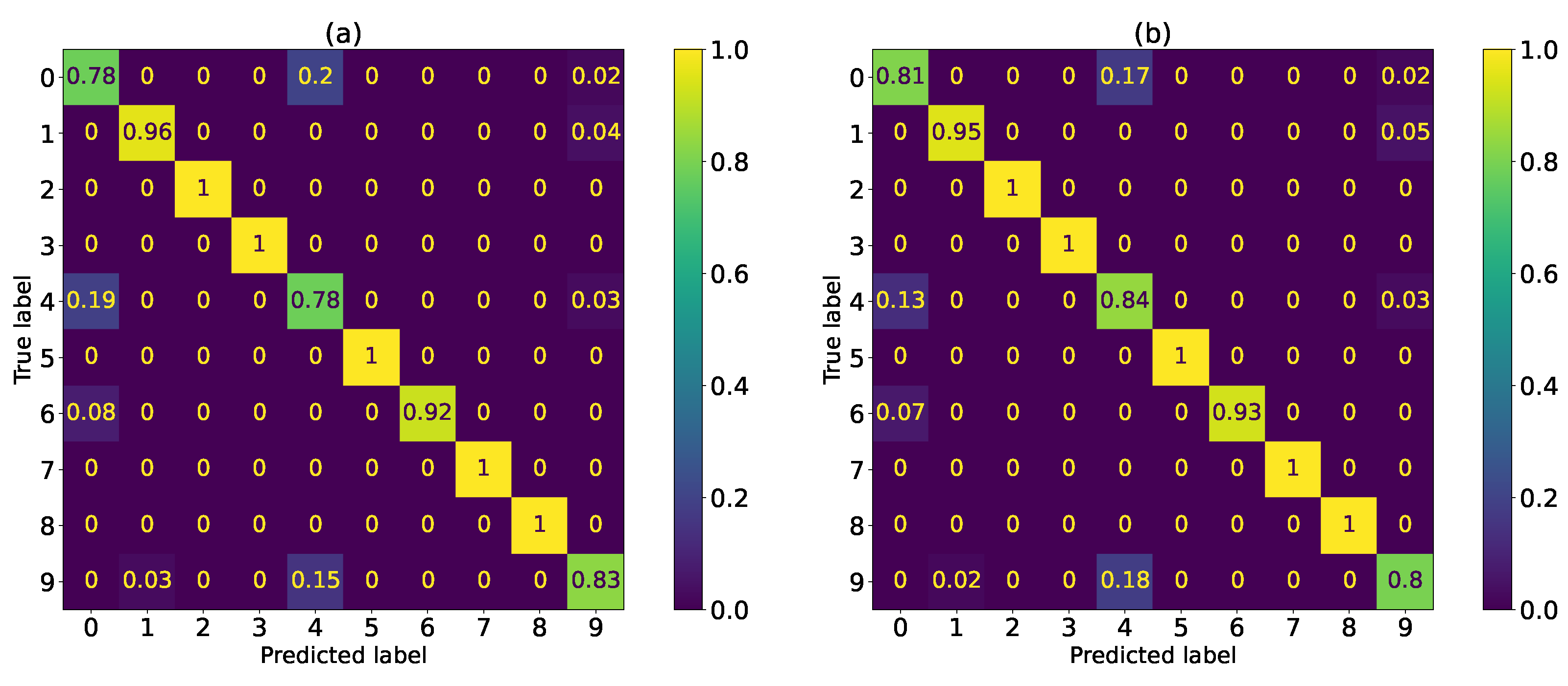
The preprocessed, simulated data set with 300 samples per state is then used to train a neural network with the highest possible generalization. The inputs to the neural network are the preprocessed frequency spectra of the three stator currents (see Figure 7), and the outputs are the probabilities for each of the ten fault types. The goal of the training process is to keep the loss of the test data lower than the loss of the training data. This is accomplished by manually tuning the hyperparameters of the neural network. The final hyperparameters are summarized in

Table 4. Tuned hyperparameters of the neural network with high generalization.

Hyperparameter	Values
Hidden layers	3
Number of neurons	[100, 50, 25]
Learning rate	0.001
Dropout	0.25
L1 regularization	0
L2 regularization	0.2
Batch size	32
Epochs	150

. For the training data (loss = 1.1458, accuracy = 92.7%) and the test data (loss = 1.1455, accuracy = 93.3%), the confusion matrices are obtained from Figure 9.

It can be seen that most faults can be classified with an accuracy of almost 100%. However, the neural network has difficulty in distinguishing between the cases of healthy state, broken bar, mixed eccentricity, and global bearing fault. This is due to their high similarity and the small deviation of these faults from the healthy state. In addition, the characteristics of these fault cases are highly dependent on the values of the identified parameters, such as the air gap thickness, the moment of inertia and the electrical and magnetic quantities. To overcome this problem, the parameter identification and data set creation are performed several times. This has the advantage that different sets of parameters are identified, preventing the neural network from focusing on the characteristics of a single set of parameter values. In addition, the repeated parameter identification multiplies the overall size of the data set. The neural network is trained again with a data set simulated on the basis of 10 different parameter sets (3000 samples per state in total), overcoming the previous problems. The corresponding confusion matrices in Figure 10 show that all fault cases can now be classified with an accuracy of over 90% (overall accuracy for training data: 96.9%, for test data: 96.6%).

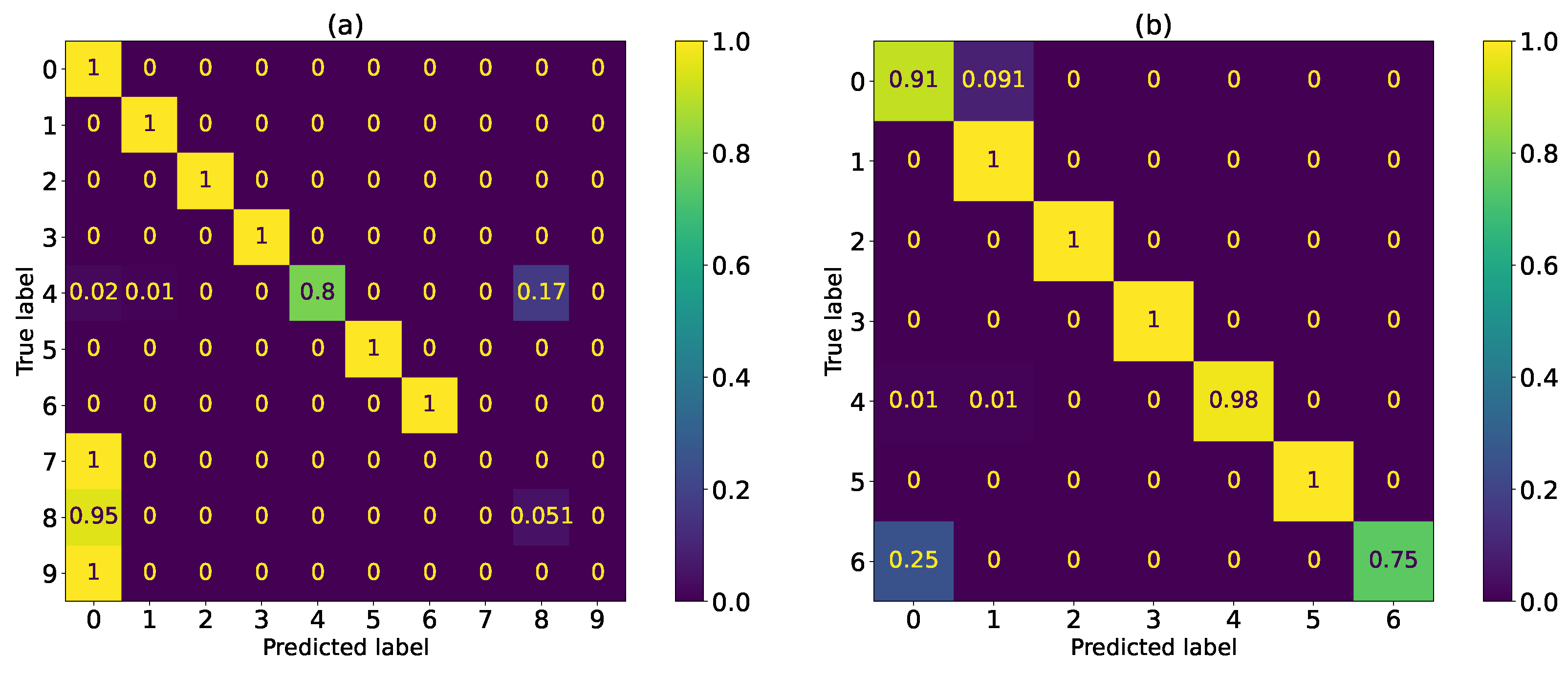
To verify the trained neural network, the same preprocessing is applied to the measured validation data. The only difference is that the normalization of the data set is now accomplished by a subtraction based on the fingerprint measurement. When the neural network is applied to the validation data, the results turn out differently depending on the fault case as can be seen on the left confusion matrix in Figure 11. It is not possible to detect the three types of bearing faults. They are classified as healthy state. This is due to the fact that the measured deviations of the bearing faults from the healthy state are marginal, and furthermore, the fault features cannot be suitably represented by the modeling. The classification of the remaining fault cases works very well with an overall detection rate of 97.14%. Training the neural network without the bearing faults in the data set also produces a very high accuracy with 94.81% on the validation data (see right confusion matrix in Figure 11).

6. Conclusions

The presented framework enables early detection of fault conditions in squirrel cage induction motors while providing a high degree of practicability. The contribution of this paper is a fault detection method for industrial applications with little prior knowledge of the motor and low measurement effort. By combining analytical modeling with parameter identification based on easily obtained data, the behavior of the monitored motor can be well reproduced. The data set simulated by the modeling enables a neural network to learn the characteristics of stator, rotor, mechanical, and voltage supply faults and to detect them in real measured data. This demonstrates that the transfer of the simulated fault characteristics to real fault cases is possible with the help of machine learning. A drawback is that bearing faults are not detected. Furthermore, the severity of the faults cannot be determined since only the major qualitative deviations have been examined so far.

The presented method combines the strengths of different approaches and mitigates their disadvantages. The prior knowledge about the effects of the fault cases is already included in the modeling and can be applied to the respective motor by means of the parameter identification. Thus, no costly measurements are required to train a neural network, but only the simulation of different fault cases to generate a sufficiently large data set. Possible inaccuracies of the modeling are concealed by the neural network by learning the qualitative characteristics of the fault cases. Therefore, an exact quantitative accuracy of the model is not necessary. These aspects clearly distinguish the presented method from pure model-, signal- or data-based approaches. Another unique point is the high practicability of the framework since the parameter identification with the differential evolution algorithm can be performed based on easily obtained measurement data and information from the nameplate.

Furthermore, the method offers a high degree of flexibility. On the one hand, this applies to parameter identification, where the desired parameters can be selected depending on the application. On the other hand, the modeling itself is also flexible so that for other machine types, such as doubly-fed induction generators or synchronous motors with permanent magnets, the model can be adapted accordingly, and the method can still be carried out. Thus, the presented approach offers high transferability to different motor types and applications.

Further work will apply more sophisticated machine learning methods to improve the detection accuracy. This should also strengthen the robustness and generalization for the transferability of the fault characteristics from the simulated data to real data. Additionally, a method for the independent detection of bearing faults based on acoustic or vibration data will be developed. In combination with the presented framework, this should cover the detection of several possible fault cases for squirrel cage induction motors.

References

1. Benbouzid, M.E.H. A review of induction motors signature analysis as a medium for faults detection. IEEE Trans. Ind. Electron. 2000, 47, 984–993. [Google Scholar] [CrossRef] [Green Version]
2. Bellini, A.; Filippetti, F.; Tassoni, C.; Capolino, G.-A. Advances in Diagnostic Techniques for Induction Machines. IEEE Trans. Ind. Electron. 2008, 55, 142–149. [Google Scholar] [CrossRef]
3. Zhang, P.; Du, Y.; Habetler, T.G.; Lu, B. A Survey of Condition Monitoring and Protection Methods for Medium-Voltage Induction Motors. IEEE Trans. Ind. Appl. 2011, 55, 34–46. [Google Scholar] [CrossRef]
4. Gao, Z.; Cecati, C.; Ding, S.X. A Survey of Fault Diagnosis and Fault-Tolerant Techniques—Part I: Fault Diagnosis With Model-Based and Signal-Based Approaches. IEEE Trans. Ind. Electron. 2015, 62, 3757–3767. [Google Scholar] [CrossRef] [Green Version]
5. Benbouzid, M.E.H.; Vieira, M.; Theys, C. Induction motors’ faults detection and localization using stator current advanced signal processing techniques. IEEE Trans. Power Electron. 1999, 14, 14–22. [Google Scholar] [CrossRef]
6. Thomson, W.T.; Fenger, M. Current signature analysis to detect induction motor faults. IEEE Ind. Appl. Mag. 2001, 7, 26–34. [Google Scholar] [CrossRef]
7. Jung, J.-H.; Lee, J.-J.; Kwon, B.-H. Online Diagnosis of Induction Motors Using MCSA. IEEE Trans. Ind. Electron. 2006, 53, 1842–1852. [Google Scholar] [CrossRef]
8. Cruz, S.M.A.; Cardoso, A.J.M. Stator winding fault diagnosis in three-phase synchronous and asynchronous motors, by the extended Park’s vector approach. IEEE Trans. Ind. Appl. 2001, 37, 1227–1233. [Google Scholar] [CrossRef]
9. Cardoso, M.A.; Cruz, S.M.A.; Fonseca, D.S.B. Inter-turn stator winding fault diagnosis in three-phase induction motors, by Park’s vector approach. IEEE Trans. Energy Convers. 1999, 14, 595–598. [Google Scholar] [CrossRef]
10. CusidÓCusido, J.; Romeral, L.; Ortega, J.A.; Rosero, J.A.; Espinosa, A.G. Fault Detection in Induction Machines Using Power Spectral Density in Wavelet Decomposition. IEEE Trans. Ind. Electron. 2008, 55, 633–643. [Google Scholar] [CrossRef]
11. Bouzida, A.; Touhami, O.; Ibtiouen, R.; Belouchrani, A.; Fadel, M.; Rezzoug, A. Fault Diagnosis in Industrial Induction Machines Through Discrete Wavelet Transform. IEEE Trans. Ind. Electron. 2001, 37, 1227–1233. [Google Scholar] [CrossRef]
12. Zamudio-Ramirez, I.; Antonino-Daviu, J.A.; Osornio-Rios, R.A.; de Jesus Romero-Troncoso, R.; Razik, H. Detection of Winding Asymmetries in Wound-Rotor Induction Motors via Transient Analysis of the External Magnetic Field. IEEE Trans. Ind. Electron. 2020, 67, 5050–5059. [Google Scholar] [CrossRef]
13. Climente-Alarcon, V.; Antonino-Daviu, J.A.; Riera-Guasp, M.; Puche-Panadero, R.; Escobar, L. Application of the Wigner—Ville distribution for the detection of rotor asymmetries and eccentricity through high-order harmonics. Electr. Power Syst. Res. 2012, 91, 28–36. [Google Scholar] [CrossRef]
14. Soualhi, A.; Medjaher, K.; Zerhouni, N. Bearing health monitoring based on hilbert huang transform, support vector machine, and regression. IEEE Trans. Instrum. Meas. 2015, 64, 52–62. [Google Scholar] [CrossRef] [Green Version]
15. Benbouzid, M.E.H.; Kliman, G.B. What stator current processing-based technique to use for induction motor rotor faults diagnosis? IEEE Trans. Energy Convers. 2003, 18, 238–244. [Google Scholar] [CrossRef] [Green Version]
16. Henao, H.; Capolino, G.-A.; Fernandez-Cabanas, M.; Filippetti, F.; Bruzzese, C.; Strangas, E.; Pusca, R.; Estima, J.; Riera-Guasp, M.; Hedayati-Kia, S. Trends in Fault Diagnosis for Electrical Machines: A Review of Diagnostic Techniques. IEEE Ind. Electron. Mag. 2014, 8, 31–42. [Google Scholar] [CrossRef]
17. Dorrell, D.G.; Thomson, W.T.; Roach, S. Analysis of airgap flux, current, and vibration signals as a function of the combination of static and dynamic airgap eccentricity in 3-phase induction motors. IEEE Trans. Ind. Appl. 1997, 33, 24–34. [Google Scholar] [CrossRef]
18. Immovilli, F.; Bellini, A.; Rubini, R.; Tassoni, C. Diagnosis of Bearing Faults in Induction Machines by Vibration or Current Signals: A Critical Comparison. IEEE Trans. Ind. Appl. 2010, 46, 1350–1359. [Google Scholar] [CrossRef]
19. Henao, H.; Demian, C.; Capolino, G.-A. A frequency-domain detection of stator winding faults in induction machines using an external flux sensor. IEEE Trans. Ind. Appl. 2003, 39, 1272–1279. [Google Scholar] [CrossRef]
20. Park, Y.; Choi, H.; Shin, J.; Park, J.; Lee, S.B.; Jo, H. Airgap Flux Based Detection and Classification of Induction Motor Rotor and Load Defects During the Starting Transient. IEEE Trans. Ind. Electron. 2020, 67, 10075–10084. [Google Scholar] [CrossRef]
21. Zamudio-Ramírez, I.; Osornio-Rios, R.A.; Antonino-Daviu, J.A. Smart Sensor for Fault Detection in Induction Motors Based on the Combined Analysis of Stray-Flux and Current Signals: A Flexible, Robust Approach. IEEE Ind. Appl. Mag. 2022, 28, 56–66. [Google Scholar] [CrossRef]
22. Choudhary, A.; Goyal, D.; Letha, S.S. Infrared Thermography-Based Fault Diagnosis of Induction Motor Bearings Using Machine Learning. IEEE Sensors J. 2021, 21, 1727–1734. [Google Scholar] [CrossRef]
23. Choudhary, A.; Mian, T.; Fatima, S.; Panigrahi, B.K. Passive Thermography Based Bearing Fault Diagnosis Using Transfer Learning With Varying Working Conditions. IEEE Sensors J. 2023, 23, 4628–4637. [Google Scholar] [CrossRef]
24. Joksimovic, G.M.; Penman, J. The detection of inter-turn short circuits in the stator windings of operating motors. IEEE Trans. Ind. Electron. 2000, 47, 1078–1084. [Google Scholar] [CrossRef]
25. Tallam, R.M.; Habetler, T.G.; Harley, R.G. Transient model for induction machines with stator winding turn faults. IEEE Trans. Ind. Appl. 2002, 38, 632–637. [Google Scholar] [CrossRef]
26. Kliman, G.B.; Koegl, R.A.; Stein, J.; Endicott, R.D.; Madden, M.W. Noninvasive detection of broken rotor bars in operating induction motors. IEEE Trans. Energy Convers. 1988, 3, 873–879. [Google Scholar] [CrossRef]
27. Bellini, A.; Filippetti, F.; Franceschini, G.; Tassoni, C.; Kliman, G.B. Quantitative evaluation of induction motor broken bars by means of electrical signature analysis. IEEE Trans. Ind. Appl. 2001, 37, 1248–1255. [Google Scholar] [CrossRef]
28. Nandi, S.; Ahmed, S.; Toliyat, H.A. Detection of rotor slot and other eccentricity related harmonics in a three phase induction motor with different rotor cages. IEEE Trans. Energy Convers. 2001, 16, 253–260. [Google Scholar] [CrossRef]
29. Schoen, R.R.; Habetler, T.G.; Kamran, F.; Bartfield, R.G. Motor bearing damage detection using stator current monitoring. IEEE Trans. Ind. Appl. 1995, 31, 1274–1279. [Google Scholar] [CrossRef]
30. Blodt, M.; Granjon, P.; Raison, B.; Rostaing, G. Models for Bearing Damage Detection in Induction Motors Using Stator Current Monitoring. IEEE Trans. Ind. Electron. 2008, 55, 1813–1822. [Google Scholar] [CrossRef] [Green Version]
31. Filippetti, F.; Franceschini, G.; Tassoni, C.; Vas, P. AI techniques in induction machines diagnosis including the speed ripple effect. IEEE Trans. Ind. Appl. 1998, 34, 98–108. [Google Scholar] [CrossRef]
32. Riera-Guasp, M.; Antonino-Daviu, J.A.; Capolino, G.-A. Advances in Electrical Machine, Power Electronic, and Drive Condition Monitoring and Fault Detection: State of the Art. IEEE Trans. Ind. Electron. 2015, 62, 1746–1759. [Google Scholar] [CrossRef]
33. Filippetti, F.; Franceschini, G.; Tassoni, C.; Vas, P. Recent developments of induction motor drives fault diagnosis using AI techniques. IEEE Trans. Ind. Electron. 2000, 47, 994–1004. [Google Scholar] [CrossRef]
34. Singh, M.; Shaik, A.G. Incipient Fault Detection in Stator Windings of an Induction Motor Using Stockwell Transform and SVM. IEEE Trans. Instrum. Meas. 2020, 69, 9496–9504. [Google Scholar] [CrossRef]
35. Ali, M.Z.; Shabbir, M.N.S.K.; Liang, X.; Zhang, Y.; Hu, T. Machine learningbased fault diagnosis for single- and multi-faults in induction motors using measured stator currents and vibration signals. IEEE Trans. Ind. Appl. 2019, 55, 2378–2391. [Google Scholar] [CrossRef]
36. Ibrahim, A.; Anayi, F.; Packianather, M.; Alomari, O.A. New Hybrid Invasive Weed Optimization and Machine Learning Approach for Fault Detection. Energies 2022, 15, 1488. [Google Scholar] [CrossRef]
37. Su, H.; Chong, K.T. Induction machine condition monitoring using neural network modeling. IEEE Trans. Ind. Electron. 2007, 54, 241–249. [Google Scholar] [CrossRef]
38. Schoen, R.R.; Lin, B.K.; Habetler, T.G.; Schlag, J.H.; Farag, S. An unsupervised, on-line system for induction motor fault detection using stator current monitoring. IEEE Trans. Ind. Appl. 1995, 31, 1280–1286. [Google Scholar] [CrossRef]
39. Martins, J.F.; Pires, V.F.; Pires, A.J. Unsupervised neural-network-based algorithm for an on-line diagnosis of three-phase induction motor stator fault. IEEE Trans. Ind. Electron. 2007, 54, 259–264. [Google Scholar] [CrossRef]
40. Ince, T.; Kiranyaz, S.; Eren, L.; Askar, M.; Gabbouj, M. Real-Time Motor Fault Detection by 1-D Convolutional Neural Networks. IEEE Trans. Ind. Electron. 2016, 63, 7067–7075. [Google Scholar] [CrossRef]
41. Sun, W.; Zhao, R.; Yan, R.; Shao, S.; Chen, X. Convolutional discriminative feature learning for induction motor fault diagnosis. IEEE Trans. Ind. Inform. 2017, 13, 1350–1359. [Google Scholar] [CrossRef]
42. Zhao, R.; Wang, D.; Yan, R.; Mao, K.; Shen, F.; Wang, J. Machine Health Monitoring Using Local Feature-Based Gated Recurrent Unit Networks. IEEE Trans. Ind. Electron. 2018, 65, 1539–1548. [Google Scholar] [CrossRef]
43. Zhao, R.; Wang, J.; Yan, R.; Mao, K. Machine health monitoring with lstm networks. In Proceedings of the 2016 10th International Conference on Sensing Technology (ICST), Nanjing, China, 11–13 November 2016; pp. 1–6. [Google Scholar]
44. Sun, J.; Yan, C.; Wen, J. Intelligent bearing fault diagnosis method combining compressed data acquisition and deep learning. IEEE Trans. Instrum. Meas. 2018, 67, 185–195. [Google Scholar] [CrossRef]
45. Chen, Z.; Li, W. Multisensor Feature Fusion for Bearing Fault Diagnosis Using Sparse Autoencoder and Deep Belief Network. IEEE Trans. Instrum. Meas. 2017, 66, 1693–1702. [Google Scholar] [CrossRef]
46. Seshadrinath, J.; Singh, B.; Panigrahi, B.K. Vibration analysis based interturn fault diagnosis in induction machines. IEEE Trans. Ind. Inform. 2014, 10, 340–350. [Google Scholar] [CrossRef]
47. Husari, F.; Seshadrinath, J. Incipient Interturn Fault Detection and Severity Evaluation in Electric Drive System Using Hybrid HCNN-SVM Based Model. IEEE Trans. Ind. Inform. 2022, 18, 1823–1832. [Google Scholar] [CrossRef]
48. Nejjari, H.; Benbouzid, M.E.H. Monitoring and diagnosis of induction motors electrical faults using a current park’s vector pattern learning approach. IEEE Trans. Ind. Appl. 2000, 36, 730–735. [Google Scholar] [CrossRef]
49. Martinez-Herrera, A.L.; Ferrucho-Alvarez, E.R.; Ledesma-Carrillo, L.M.; Mata-Chavez, R.I.; Lopez-Ramirez, M.; Cabal-Yepez, E. Multiple Fault Detection in Induction Motors through Homogeneity and Kurtosis Computation. Energies 2022, 15, 1541. [Google Scholar] [CrossRef]
50. Tran, M.-Q.; Liu, M.-K.; Tran, Q.-V.; Nguyen, T.-K. Effective Fault Diagnosis Based on Wavelet and Convolutional Attention Neural Network for Induction Motors. IEEE Trans. Instrum. Meas. 2022, 71, 1–13. [Google Scholar] [CrossRef]
51. Guo, X.; Chen, L.; Shen, C. Hierarchical adaptive deep convolution neural network and its application to bearing fault diagnosis. Measurement 2016, 93, 490–502. [Google Scholar] [CrossRef]
52. Zhang, S.; Zhang, S.; Wang, B.; Habetler, T.G. Deep Learning Algorithms for Bearing Fault Diagnostics—A Comprehensive Review. IEEE Access 2020, 8, 29857–29881. [Google Scholar] [CrossRef]
53. Murphey, Y.L.; Masrur, M.A.; Chen, Z.; Zhang, B. Model-based fault diagnosis in electric drives using machine learning. IEEE/ASME Trans. Mechatr. 2006, 11, 290–303. [Google Scholar] [CrossRef]
54. Masrur, M.A.; Chen, Z.; Zhang, B.; Murphey, Y.L. Model-based fault diagnosis in electric drive inverters using artificial neural network. In Proceedings of the 2007 IEEE Power Engineering Society GeneralMeeting, Tampa, FL, USA, 24–28 June 2007; pp. 1–7. [Google Scholar]
55. Nürnberg, W.; Hanitsch, W. Die Prüfung Elektrischer Maschinen; Springer: Berlin/Heidelberg, Germany, 1987. [Google Scholar]
56. International Electrotechnical Commission (IEC). IEC 60034-28:2012; Rotating Electrical Machines—Part 28: Test Methods for Determining Quantities of Equivalent Circuit Diagrams for Three-Phase Low-Voltage Cage Induction Motors. IEC: Geneva, Switzerland, 2012.
57. Rosendahl, J. Ursachen und Auswirkungen von Windungs- und Phasenschlüssen im Stator Großer Synchronmaschinen; Shaker: Aachen, Germany, 2010. [Google Scholar]
58. Krause, P.; Wasynczuk, O.; Sudhoff, S.; Pekarek, S. Analysis of Electric Machinery and Drive Systems; Wiley-IEEE Press: Hoboken, NJ, USA, 2013. [Google Scholar]
59. Lubin, T.; Hamiti, T.; Razik, H.; Rezzoug, A. Comparison between finite-element analysis and winding function theory for inductances and torque calculation of a synchronous reluctance machine. IEEE Trans. Magn. 2007, 43, 3406–3410. [Google Scholar] [CrossRef] [Green Version]
60. Nandi, S.; Bharadwaj, R.; Toliyat, H. Performance analysis of a three-phase induction motor under mixed eccentricity condition. IEEE Trans. Energy Convers. 2002, 17, 392–399. [Google Scholar] [CrossRef]
61. Toliyat, H.; Lipo, T.; White, J. Analysis of a concentrated winding induction machine for adjustable speed drive applications. i. motor analysis. IEEE Trans. Energy Convers. 1991, 6, 679–683. [Google Scholar] [CrossRef]
62. Toliyat, H.A.; Lipo, T.A. Transient analysis of cage induction machines under stator, rotor bar and end ring faults. IEEE Trans. Energy Convers. 1995, 10, 241–247. [Google Scholar] [CrossRef] [Green Version]
63. Luo, X.; Liao, Y.; Toliyat, H.; El-Antably, A.; Lipo, T. Multiple coupled circuit modeling of induction machines. IEEE Trans. Ind. Appl. 1995, 31, 311–318. [Google Scholar]
64. Al-Nuaim, N.; Toliyat, H. A novel method for modeling dynamic air-gap eccentricity in synchronous machines based on modified winding function theory. IEEE Trans. Energy Convers. 1998, 13, 156–162. [Google Scholar] [CrossRef] [Green Version]
65. Tang, J.; Chen, J.; Dong, K.; Yang, Y.; Lv, H.; Liu, Z. Modeling and Evaluation of Stator and Rotor Faults for Induction Motors. Energies 2020, 13, 133. [Google Scholar] [CrossRef] [Green Version]
66. Storn, R.; Price, K. Differential Evolution—A Simple and Efficient Heuristic for global optimization over Continuous Spaces. J. Glob. Optim. 1997, 11, 341–359. [Google Scholar] [CrossRef]
67. Kochenderfer, M.J.; Wheeler, T.A. Algorithms for Optimization; MIT Press: Cambridge, MA, USA, 2019. [Google Scholar]
68. Storn, R. On the usage of differential evolution for function optimization. In Proceedings of the North American Fuzzy Information Processing, Berkeley, CA, USA, 19–22 June 1996; pp. 519–523. [Google Scholar]
69. Rumelhart, D.E.; Hinton, G.E.; Williams, R.J. Learning representations by back-propagating errors. Nature 1986, 323, 533–536. [Google Scholar] [CrossRef]
70. Bishop, C.M. Neural Networks for Pattern Recognition; Oxford University Press: Oxford, UK, 1995. [Google Scholar]
71. Goodfellow, I.; Bengio, Y.; Courville, A. Deep Learning; MIT Press: Cambridge, MA, USA, 2016. [Google Scholar]
72. LeCun, Y.; Bengio, Y.; Hinton, G. Deep learning. Nature 2015, 521, 436–444. [Google Scholar] [CrossRef]
73. Ng, A. Feature selection, L1 vs. L2 regularization, and rotational invariance. In Proceedings of the Twenty-First International Conference on Machine Learning, Banff, AB, Canada, 4–8 July 2004. [Google Scholar]
74. Srivastava, N.; Hinton, G.; Krizhevsky, A.; Sutskever, I.; Salakhutdinov, R. Dropout: A simple way to prevent neural networks from overfitting. J. Mach. Learn. Res. 2014, 1, 1929–1958. [Google Scholar]
Figure 1. Electrical network of a rotor of a squirrel cage induction motor with the individual loop currents i R , end ring current i E , and associated resistances R e and R b , as well as leakage inductances L e and L b of cage bars and end ring segments.
Energies 16 03429 g001
Figure 2. Electrical network of a stator of a squirrel cage induction motor with the phase currents i S and the winding short-circuit path (red) with short-circuit current i K and the resistor R K .
Energies 16 03429 g002
Figure 3. Electrical network of a rotor of a squirrel cage induction motor with the individual loop currents i R in case of one broken cage bar.
Energies 16 03429 g003
Figure 4. Structure of multiple coupled circuit modeling with inputs (voltages U S and load torque T L ) and outputs (stator currents i S and rotor speed ω ).
Energies 16 03429 g004
Figure 5. Sequence of the individual steps of the fault detection framework up to the application with real measurement data.
Energies 16 03429 g005
Figure 6. Sequence of the individual steps of the parameter identification from the fingerprint measurement (startup process from standstill to rated operation) and nameplate data to the identification process.
Energies 16 03429 g006
Figure 7. Sequence of the individual steps of the preprocessing with fast Fourier transformation, clipping, and normalization via the subtraction with the healthy state.
Energies 16 03429 g007
Figure 8. Comparison of the frequency spectra for one of the three stator currents from the fingerprint measurement and the simulation with the parameterized model: (a) complete frequency spectrum; (b) zoom of the frequency spectrum into the significant range (0 to 1000 Hz).
Energies 16 03429 g008
Figure 9. Confusion matrix with results of accuracy for each fault case for the training data (a) and test data (b). 0: healthy state; 1: undervoltage; 2: unsymmetrical voltage; 3: open phase; 4: broken bar; 5: winding short circuit; 6: mixed eccentricity; 7: bearing—outer ring fault; 8: bearing—inner ring fault; 9: bearing—global fault.
Energies 16 03429 g009
Figure 10. Confusion matrix with results of accuracy for each fault case for the training data (a) and test data (b) with 10 different parameter sets. 0: healthy state; 1: undervoltage; 2: unsymmetrical voltage; 3: open phase; 4: broken bar; 5: winding short circuit; 6: mixed eccentricity; 7: bearing—outer ring fault; 8: bearing—inner ring fault; 9: bearing—global fault.
Energies 16 03429 g010
Figure 11. Confusion matrix with results of accuracy for each fault case for the validation data (a) and validation data without bearing faults (training data also without bearing faults) (b). 0: Healthy state; 1: undervoltage; 2: unsymmetrical voltage; 3: open phase; 4: broken bar; 5: winding short circuit; 6: mixed eccentricity; 7: bearing—outer ring fault; 8: bearing—inner ring fault; 9: bearing—global fault.
Energies 16 03429 g011