Abstract
An electrical power system (EPS) is subject to unexpected events that might cause the outage of elements such as transformers, generators, and transmission lines. For this reason, the EPS should be able to withstand the failure of one of these elements without changing its operational characteristics; this operativity functionality is called contingency. This paper proposes a methodology for the optimal location and sizing of a parallel static Var compensator (SVC) in an EPS to reestablish the stability conditions of the system before contingencies take place. The system’s stability is analyzed using the fast voltage stability index (FVSI) criterion, and the optimal SVC is determined by also considering the lowest possible cost. This research considers contingencies involving the disconnection of transmission lines. Then, the methodology analyzes every scenario in which a transmission line is disconnected. For every one of them, the algorithm finds the weakest transmission line by comparing FVSI values (the higher the FVSI, the closer the transmission line is to instability); afterward, when the weakest line is selected, by brute force, an SVC with values of 5 Mvar to 100 Mvars in steps of 5 Mvar is applied to the sending bus bar of this transmission line. Then, the SVC value capable of reestablishing each line’s FVSI to its pre-contingency value while also reestablishing each bus-bar’s voltage profile and having the lowest cost is selected as the optimal solution. The proposed methodology was tested on IEEE 14, 30, and 118 bus bars as case studies and was capable of reestablishing the FVSI in each contingency to its value prior to the outage, which indicates that the algorithm performs with 100% accuracy. Additionally, voltage profiles were also reestablished to their pre-contingency values, and in some cases, they were even higher than the original values. Finally, these results were achieved with a single solution for a unique SVC located in one bus bar that is capable of reestablishing operational conditions under all possible contingency scenarios.
1. Introduction
In an electrical power system (EPS), certain aspects, such as planning, operation, management, and expansion, are essential for optimal EPS performance.
Among management issues, energy management is especially important. Some research articles have considered an intelligent framework for energy management in hybrid AC-DC microgrids with renewable energy sources and storage devices as a strategy for smart energy management [1].
As for expansion, nowadays, the increasing development of offshore wind farms is a new trend in the wind power industry due to benefits such as stable wind speed and their renewable and non-polluting nature, and the ability to avoid occupying cultivated land is highly sought in the electrical industry [2].
However, among the previously indicated EPS stages, voltage stability is an important issue that must be considered to ensure the safe and economical delivery of electrical energy to end users.
The traditional EPS faces challenges in its stability due to the occurrence of changes, especially in the transmission system, such as the continuous increase in electrical load and the growing incorporation of renewable energy sources. Excessive load on transmission lines is a crucial challenge for the power grid, as it can cause severe voltage drops and eventual system collapse in the case of an overload. Even minor disturbances can lead the grid to a critical state in such circumstances.
To date, research in the literature has focused on studying different stability indices in transmission lines and nodes to predict system collapse, establish appropriate strategies for load shedding due to voltage instabilities, regulate the load capacity of transmission lines, and reduce losses through reactive compensation systems.
This paper presents a methodology that improves power system stability by installing static VARS compensators (SVCs) according to the fast voltage stability index under contingency scenarios while also considering costs and the improvement of voltage profiles.
1.1. Literature Review
Voltage stability is one of the most studied parameters of EPSs. For instance, ref. [3] describes voltage stability indices such as BVCPI, FVSI, LQP, BVCPI, and VCP-1. This review focuses on indices that identify the weakest bus in the electrical network and the application of PSO to minimize losses that cause voltage instability. The paper begins with a detailed understanding of blackouts and the phenomenon of voltage instability/stability, the classification of power systems, and corresponding formulations. The study provides an overview of voltage assessment techniques before applying PSO for discrete and multi-objective optimization and their advantages over other techniques.
The study in [4] compared and evaluated six voltage stability indices, namely, Lmn, FVSI, LQP, Lp, NVSI, and NLSI_1, and tested their effectiveness through numerical studies in the IEEE 14-bus test system under various loading conditions. The research in [4] aimed to identify the most suitable index to monitor the Nigerian power system. The advantages and disadvantages of each index are presented, and their performance was assessed in terms of their ability to predict voltage stability. The results provide insights into the strengths and weaknesses of each index and enable the selection of an appropriate index for monitoring the Nigerian power system.
The voltage stability of an electrical network is crucial to avoiding blackouts. It is achieved by identifying the system’s weak and less reliable elements by calculating their stability indices, whether in nodes or in lines [5]. Evaluating system stability and identifying weak elements are fundamental to reliable operation and uninterrupted supply. For example, in the study in [6], two approaches were evaluated to identify weak buses: the previously developed fast voltage stability index and a new reduced index based on fuzzy logic proposed by the authors; the classical approach based on the reduced method calculates contingencies more accurately and produces reliable results.
In [7], it was demonstrated that node-based indices are superior to line-based indices in identifying weak nodes and areas in power systems that are susceptible to instabilities. The research in [8] proposes a practical methodology based on Artificial Neural Networks to predict the fast voltage stability index. The proposed method was tested on IEEE 14- and IEEE 30-bus test systems. A comparative analysis of different RNA topologies was carried out based on the FVSI prediction capability, and the results were validated using the offline Newton–Raphson simulation method.
Voltage collapse is a critical consequence of voltage instability, which occurs when power systems operate at their maximum power transfer capacity limits. Therefore, it is essential to evaluate and, above all, have an accurate estimate of critical operating conditions to prevent voltage collapse through various indices that allow for the close monitoring of the system and the precise prediction of voltage collapse so that system technicians and operators can take timely corrective measures and ensure a more reliable and secure electrical network. This has led some authors to focus on calculating and, in some cases, proposing new stability indicators and comparing them with traditional ones for stability evaluation, as in [9,10], where two new modern indices for voltage stability evaluation (MVSI and NCPI) are presented and compared with indices such as Lmn, FVSI, LQP, NLSI, and VSLI. Their results show that these indices effectively identify critical lines, weak buses, and areas in medium to large networks under various operating conditions, including contingencies, with Mokred validating their proposal in the IEEE 30-bus system. Additionally, in [11], the focus is on the usefulness of two voltage stability indices (FVSI and LQP) to identify weak buses so that appropriate measures can be taken in advance to prevent voltage collapse.
In the two studies described in [12,13], a new line stability index (NLSI_1) is proposed to predict voltage collapse in electrical power systems. It is based on a switching logic derived from the voltage angle difference between the loads of the evaluated nodes. The results are compared with the line stability index (Lmn) and the fast voltage stability index (FVSI) in the IEEE 14-bus test system and a real case of the Nigerian network.
The research in [14] discusses the evaluation of the maximum loadability of the transmission network, considering single and double contingencies. To achieve this, the installation of SVC, TCSC, and UPFC devices is considered, increasing the power transfer capability. The methodology for identifying the appropriate point to compensate is based on evaluating stability indices such as the CSI and FVSI. The proposed problem was simulated using MATLAB 7.0 and tested with the WSCC 9-bus system, optimizing with the MDE algorithm. The results show that the method reduces installation costs and improves the overloading of transmission lines.
Reactive compensation is one of the best ways to improve the steady-state operation of a power system. For example, in [15], the system’s operability and reliability were enhanced by optimizing the placement and sizing of FACTS-based compensation systems to reduce voltage deviation in 14-, 30-, and 118-bus test systems while accounting for uncertainty in demand growth using deep neural networks. However, these works did not consider the power system’s voltage stability [16].
The researchers in [17] propose the use of voltage stability indices to monitor and control the voltage of an electric power system and propose a method for the optimal placement of a series static synchronous compensator (SSSC) to improve voltage stability. The technique involves classifying contingencies according to their voltage stability margins, analyzing three voltage stability indices under the five main contingencies, and placing the SSSC on the five main critical lines to observe the optimal placement. The proposed method was applied to an IEEE 14-bus system, and the results show that the SSSC improves the voltage stability of the system.
The authors of [18] presents a new methodology for the optimal installation of Distribution Static Compensators (DSTATCOMs) in Electric Distribution Systems (EDSs) using an Arithmetic Optimization Algorithm (AOA). The objective of the methodology is to minimize the active energy loss (APL) and various voltage stability indices, including the voltage stability index (VSI), fast voltage stability index (FVSI), line stability factor (LPQ), and power/voltage stability index (PVSI). The methodology was tested on 33- and 69-bus systems, and the results show that the optimal installation of the DSTATCOM can significantly reduce energy losses and improve voltage profiles.
In [19], the researchers present a method for optimizing shunt compensation in electric power systems to improve voltage stability. FVSIs are used to determine vulnerable load lines and buses, while PSO is used to find a shunt compensator’s optimal location and size. The method was applied to the IEEE 14-bus test system for different contingencies, and the results show an improvement in voltage stability. The methodology used in this study consists of two main steps: First, FVSIs are used to identify vulnerable load buses and lines in the electric power system. Then, the PSO algorithm is used to find the optimal location and size of shunt compensators. A STATCOM was implemented as a shunt compensator. The study results show that implementing the proposed method significantly improves the electrical power system’s voltage stability and load capacity. Furthermore, the study demonstrates that using FVSIs and the PSO algorithm optimizes shunt compensation in electric power systems. The main contribution of this study is the proposal of an effective method for optimizing shunt compensation in electric power systems using FVSIs and the PSO algorithm.
By installing SVC and TCSC FACTS devices on the weakest bus and line, the study in [20] shows how to increase the energy transfer, voltage profile, and load capacity. It also examines using FACTS devices to reduce overload in electric power transmission networks. They used the standard IEEE 30-bus test system to validate their methods. The findings indicate that using FACTS devices improves the voltage profile, energy transfer, and load capacity and reduces energy loss. The employment of FACTS devices has also been shown to considerably increase the performance of the electric power system, which has significant implications for the electric power sector.
The study shown in [21] discusses the issue of the voltage stability of electric power networks and suggests using two indices, the line stability index (Lmn) and fast voltage stability index (FVSI), for an IEEE 30-bus test system to identify the weakest bus. The findings demonstrate that shunt compensation is the most effective FACTS compensator for increasing voltage stability. Tables and figures are used to support the results. In conclusion, the study proposes a methodology for enhancing the voltage stability of electric power networks and presents a practical approach to identifying and addressing the system’s weakest bus.
In [22], an integrated framework for evaluating and improving the voltage stability of electric power systems through optimal load shedding is proposed. The objective is to enhance the voltage stability of electric power systems by identifying weak buses and lines and using load shedding as a control method to stabilize the system. The methodology employs various voltage stability indices to identify weak buses and lines. Optimal load shedding uses metaheuristic algorithms such as particle swarm and gray wolf optimization. The technique was successfully tested on the IEEE 30-bus test system. The results show that the proposed technique based on the FVSI is effective in improving the voltage profile under high-demand conditions. The study also highlights the advantages of using GWO instead of PSO for computational efficiency and voltage profile improvement.
In [23], an algorithm is presented to prevent the voltage instability of electrical networks by implementing an under-voltage load-shedding (UVLS) system using the indices FVSI and LSI in the IEEE 39-bus system with distributed generation. The results show that the system performance after disconnection did not differ significantly from the base case, and the voltage instability of electrical networks can be prevented by using the FVSI and LSI to determine the most unstable loads, which can be shed before the voltage further decreases.
In addition, distributed generation and renewable power plants are an essential part of today’s power grids. In [24], the authors provide an overview of the voltage stability index (VSI) as an important indicator of power system stability due to the increasing integration of renewable energy sources (RESs) into the power system, rapid load changes, and increasing power demand.
Deep learning has also been used to assess system stability. In [25], the authors suggest a deep-learning intelligent system for power system short-term voltage stability assessment (STVSA) that includes data augmentation. The method uses conditional least-squares generative adversarial network (LSGAN)-based data augmentation to increase the dataset after obtaining labeled samples from a limited dataset using semi-supervised cluster learning.
In [26], the authors discuss the potential issue of overvoltage in power grids due to the increased penetration of Photovoltaic (PV) units and proposes a long-term strategy to resolve the issue. The strategy involves employing demand response (DR) programs and load-shifting techniques to reduce voltage levels during peak hours. This reduces the need for active power curtailment and reactive power provision methods, which can limit the maximum injectable active solar power to the grid and decrease the inverters’ lifetime. The proposed approach also reduces under-voltage levels during peak times and introduces new insight into DR potential.
1.2. Organization
The organization of this paper is as follows: Section 1 discusses the different methodologies applied for the improvement of the stability of transmission lines. The different stability indices considered in the most relevant research works are also shown, emphasizing the fast voltage stability index (FVSI). Additionally, this section shows the previous research on FVSI improvement, how the results were evaluated, and the different techniques and methodologies applied.
Section 2 shows the mathematical basis for Newton–Raphson when applied to power flows and the fast voltage stability index calculations that this research used for its algorithms. This section also fully explains the implementation of the algorithm for the optimal location and sizing of the static VAR compensator for the improvement of the FVSI of a transmission system under all contingency scenarios.
Section 3 shows the optimal location and sizing of the SVC for the three case studies this paper describes. The results show the FVSI before and after implementing the methodology under all contingencies, and voltage profiles are treated as an analysis indicator. Finally, this section provides a detailed discussion and analysis of the results.
Finally, Section 4 summarizes the conclusions of the research performed in this work.
2. Methodology
This work proposes a methodology for improving the stability of electrical power systems under contingency scenarios involving the disconnection of transmission lines. For this purpose, the fast voltage stability index (FVSI) is used as the parameter that evaluates the system’s stability. Reactive compensation, specifically the static VAR compensator (SVC), is applied to the system. The optimal bus-bar location and sizing are determined by analyzing the transmission system’s electrical parameters calculated through Newton–Raphson.
Additionally, for all case studies, the system was analyzed under normal load conditions; in other words, this research did not consider increases in active or reactive loads over those already connected to the system, which will be studied in future works.
The methodology is explained in detail in the following sections, starting with concepts essential for the method proposed in this research.
2.1. Power Flow: Newton–Raphson
Different techniques are used to calculate the electrical variables of an electrical power system in a steady-state condition (power flow). Among the different methodologies, Newton–Raphson (NR) is widely used due to its fast convergence and the large region of convergence for the analyzed variables. NR is mainly based on the Jacobian matrix, a mathematical representation of the relationships and influence of voltage magnitudes V and voltage angles with variations in active and reactive power [27].
The complex power equations that are used in NR are listed below. The apparent power calculation at node i is shown in Equation (1).
Analyzing the real and imaginary terms in Equation (2) makes it possible to write expressions for real and active power, as shown in Equations (3) and (4); in these equations, the variable x refers to the unknown terms in each equation, such as , , , and .
An electrical power system needs to maintain a power balance between demanded power D and generated power G considering Equations (3) and (4); this balance is applied to both active and reactive power, as shown in Equations (5) and (6).
Then, the variables of interest to be estimated are the voltage magnitude and angle in each node, represented by Matrix (7). These variables depend on the power balance at the same nodes, represented by Matrix (8). Additionally, the voltage, angle, and power at one node are known, as this node is generally a slack bus bar.
2.2. Fast Voltage Stability Index (FVSI)
The fast voltage stability index is an indicator that evaluates the stability of a power line. This indicator has a value that varies from 0 to 1; the closer it is to 1, the closer the line is to instability. Therefore, a value closer to 0 is desired, as it indicates a more stable power line [28].
Figure 1 shows a power line connected between two bus bars: is the voltage magnitude and angle at bus bar i, is the voltage magnitude and angle at bus bar j, and line has an impedance of .
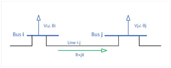
Figure 1.
Fast voltage stability index calculation between two nodes [].
Subsequently, the FVSI at power line is calculated as shown in Equation (11), where the sub-index i corresponds to the sending node, the sub-index j represents the receiving node, is the receiving reactive power at node j, is the voltage magnitude at the sending node, is the reactance of line , and is the impedance of line .
The receiving reactive power at node j is calculated by first analyzing Equation (1), where current is now considered the current that flows in line from node i to node j. However, according to Equation (11), the reactive power considered in the calculation of the FVSI flows from node j to i; this is shown in Equation (12). From this equation, and considering , and , it is possible to state an expression to calculate reactive power , which is shown in Equation (13).
2.3. Proposed Methodology for Optimal SVC Location and Sizing
This paper proposes a methodology for the optimal location of parallel reactive compensators (SVCs) based on NR power flows and considering contingencies for transmission lines; through this methodology, the most sensitive power line (using the fast voltage stability index as the stability criterion) of the electrical power system is determined for all the different contingency scenarios by studying the FVSI and aiming for this index to be as close as possible to zero (FVSI close to one indicates a line close to instability).
While maintaining the FVSI value as close as possible to zero, the methodology also aims to increase the voltage profiles of all bus bars to their values before the contingency occurred (no line disconnected). Additionally, the algorithm considers the SVC cost, as a higher capacity means, in practice, a higher cost; for this reason, this methodology finds the optimal location and sizing of the SVC with the lowest possible SVC cost while improving voltage profiles and reducing the FVSI.
Algorithm 1 details how the FVSI is calculated for every power line in an electrical power system. First, all the electrical parameters of the transmission system, such as line impedance , conductance , substance , lines’ nodes, generators, and load power, among others, are loaded into different variables; then, the Newton–Raphson power flow is calculated, and the voltage and angle for each node are saved. Then, reactive power is calculated for each line, and the for each line is saved.
| Algorithm 1: Fast voltage stability index calculation |
|
Subsequently, Algorithm 2 determines the SVC’s optimal location and sizing. First, the original parameters of the transmission system are the loads; the critical parameters for lines are saved in , and the critical parameters for buses are saved in . Then, the original FVSI for each line of the system is calculated prior to any contingency scenario.
The next step consists of generating every contingency; in other words, every scenario in which a power line is disconnected is analyzed. Each scenario’s highest FVSI is identified to determine the most critical power line in each contingency.
The fourth step applies the SVC with values from 5 Mvar to 100 Mvar in steps of 5 Mvar at node i of the weakest line previously found. For every compensation scenario, the FVSI is calculated for the entire system. Then, the first SVC value capable of generating an FVSI less than or equal to the original is selected as the optimal solution.
Finally, the optimal size of the SVC and its bus-bar location are saved for every contingency.
| Algorithm 2: Optimal SVC location and sizing |
|
2.4. Case Studies
The IEEE 14-, 30-, and 118-bus-bar systems were considered as case studies to test the proposed methodology. These systems are transmission power systems, among which the 14-bus-bar system was developed for research, and the 30- and 118-bus-bar systems are portions of real power systems located in the United States.
This paper’s methodology finds the weakest power line and a global solution for the optimal SVC location and sizing capable of ensuring that, under any contingency (where a power line is disconnected), the transmission system can operate as well as it does under normal operating conditions. This is evaluated using the FVSI and voltage profiles.
3. Analysis of Results
3.1. Case Study: IEEE 14-Bus-Bar System
When applying Algorithm 1 to the IEEE 14-bus-bar system, the FVSI is calculated for every transmission line; this first analysis establishes which power lines are closer to instability by ordering the FVSI from highest to lowest. These data can be seen in Table 1.

Table 1.
FVSI for IEEE 14-bus-bar system before contingency scenarios.
Table 1 shows that line has the greatest FVSI and, therefore, is the power line closest to instability. According to Algorithm 2, compensation should be located at node i; however, node 2 corresponds to a PV bus bar in which, by definition, the voltage profile will not change due to voltage control in this kind of bus-bar. Therefore, Algorithm 2 selects the next worst FVSI, in this case, line, in which compensation will be located at bus bar 10.
Then, when applying Algorithm 2, every power line is disconnected, all possible contingency scenarios are analyzed, and for every scenario, all FVSIs for every connected line are calculated. Figure 2 shows the data generated in all contingency scenarios. Once again, it should be noted that the FVSI varies from 0 to 1, where the closer this index is to 1, the closer the line is to instability. This figure shows the FVSI for every transmission line in every contingency analysis case. The contingency cases are ordered from the one with the highest average FVSI to the lowest, and this figure easily identifies the most critical lines in each case.
Statistical analysis was performed on the data shown in Figure 2. In Figure 3, the information on the minimum, maximum, median, and average FVSI for each contingency scenario is shown. From this graph, and similar to the analysis performed with Algorithm 1 for all contingency scenarios, the most critical ones are those in which line or line is disconnected.
Figure 3 shows every contingency analysis case, and all FVSI values are represented as box-plot diagrams. The contingency cases are ordered from the one with the highest average FVSI to the lowest, and this figure indicates how FVSI values behave without any compensation.
As shown in Figure 3, line has a maximum and average FVSI of 0.14; similarly, line has a maximum FVSI of 0.18 and an average of 0.12. These values are compared with those in Table 1, i.e., the values before contingencies occurred, which shows that line had an FVSI of 0.13 and line had an FVSI of 0.11; therefore, as expected, there is an increase in the FVSI in all contingency scenarios.
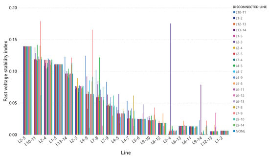
Figure 2.
Fourteen-bus-bar system: FVSI for every contingency scenario.
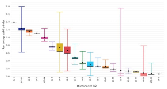
Figure 3.
Fourteen-bus-bar system: statistical analysis for every contingency scenario.
Continuing with Algorithm 2, after all contingencies are generated in step 3, step 4 applies SVC compensation with values from 5 Mvar to 100 Mvar in steps of 5 Mvar at node i of the weakest power line in every contingency case. Then, the optimal value of compensation and its location are found.
All FVSIs for every connected line when SVC compensation is connected at its optimal location and with the optimal size are shown in Figure 4. This figure shows the FVSIs for every transmission line in every contingency analysis case with the optimal solution connected. The contingency cases are ordered from the highest average FVSI to the lowest.
Similarly, Figure 5 shows the statistical analysis of the FVSI for each contingency scenario with SVC compensation. This figure shows every contingency analysis case with its optimal solution connected, and all FVSI values are represented as box-plot diagrams. The contingency cases are ordered from the highest average FVSI to the lowest.
Both Figure 4 and Figure 5 show that the FVSI at line is decreased when compared to its value without compensation.
For a global overview of the optimal SVC compensation results, Figure 6 shows the average FVSIs for all power transmission lines under every contingency scenario when a line is disconnected versus the average FVSI for every contingency scenario with its optimal (location and sizing) SVC compensator. By analyzing this information, it can be noted that the optimal location this paper proposes reduces the FVSI by 20.33%.
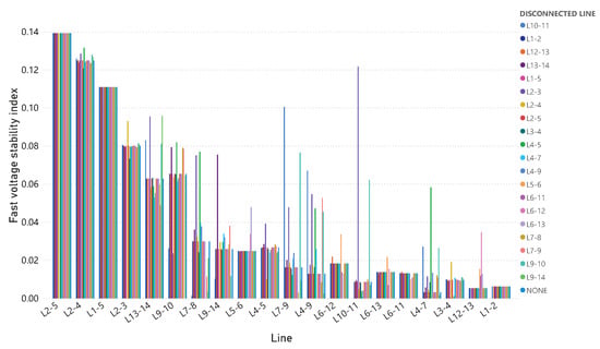
Figure 4.
Fourteen-bus-bar system: FVSIs for every contingency scenario with optimal compensation.
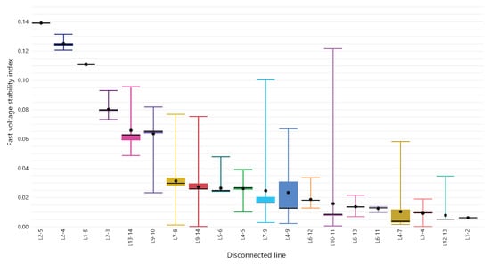
Figure 5.
Fourteen-bus-bar system: statistical analysis for every contingency scenario with optimal compensation.
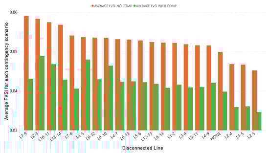
Figure 6.
Fourteen-bus-bar system: FVSI for contingencies with no compensation vs. contingencies with optimal compensation.
Results Validation
The IEEE 14-bus-bar system has 20 transmission lines; thus, there are 20 contingencies that the algorithm analyzed. For all contingency scenarios, line was selected as the weakest (highest FVSI, not considering PV buses). This paper’s methodology found that a compensation of 20 Mvar in bus bar 10 should be connected to reestablish the system’s stability as close as possible to its values before the contingencies.
From the 20 contingency scenarios, 2 have been selected to be shown and are described below.
- Contingency when the weakest line is disconnected
As can be seen in Figure 2 and Figure 3, line is the weakest under all contingency scenarios. As the results of Algorithm 2 indicate, a compensation of 20 Mvar in bus bar 10 should be connected. The FVSI values for every line before the contingency, when line is disconnected, and when the optimal compensation is connected are shown in Figure 7.
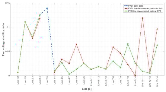
Figure 7.
First study case: FVSIs before/after contingencies and with SVC compensation, when the weakest line is disconnected.
Figure 7 shows that the optimal solution reestablished the FVSI values after the contingency occurred to their values before line was disconnected, which shows the excellent performance of the algorithm.
Similarly, for this case, voltages profiles were analyzed. Figure 8 shows the voltage profiles of all bus bars before the contingency, when line is disconnected, and when the optimal compensation is connected. This figure shows that the optimal solution reestablished the voltage profiles of all bus bars after the contingency occurred to their values before line was disconnected. These results validate the algorithm’s performance.
- Contingency when the second-weakest line is disconnected (transmission line that contains the bus bar where the SVC is located)
For the IEEE 14-bus bar system, line is the second weakest according to the results of Algorithm 2. Additionally, this scenario is crucial to analyze because the SVC is located in bus bar i from line.
The FVSI values for every line before the contingency, when line is disconnected, and when the optimal compensation is connected are shown in Figure 9. According to these results, even when the disconnected line contains the bus bar where the SVC is located, the algorithm can still reestablish the FVSI values after the contingency occurs to their values before line was disconnected.
Finally, voltages profiles were analyzed. Figure 10 shows the voltage profiles of all bus bars before the contingency, when line is disconnected, and when the optimal compensation is connected. In some cases, such as bus bars 7, 9, and 10, the voltage profiles are even higher than before the contingency, which once again validates the algorithm results.
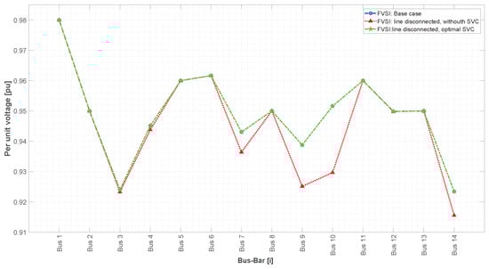
Figure 8.
First study case: Voltage profiles before/after contingencies and with SVC compensation, when the weakest line is disconnected.
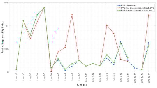
Figure 9.
First study case: FVSIs before/after contingencies and with SVC compensation, when the line that contains the node for the optimal solution is disconnected.
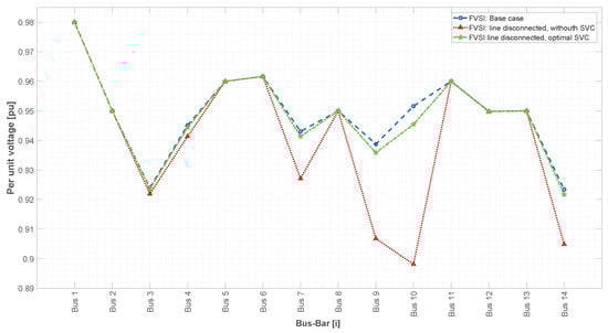
Figure 10.
First study case: Voltage profiles before/after contingencies and with SVC compensation, when the line that contains the node for the optimal solution is disconnected.
3.2. Case Study: IEEE 30-Bus-Bar System
When applying Algorithm 1 to the IEEE 30-bus-bar system, the FVSI is calculated for every transmission line; this first analysis establishes which power lines are closer to instability by ordering the FVSI from the highest to lowest. These data can be seen in Table 2.
Table 2.
FVSI for IEEE 30-bus-bar system before contingency scenarios.
Table 2 shows that line has the greatest FVSI and, therefore, is the power line closest to instability. According to Algorithm 2, compensation should be located at node i; however, node 2 corresponds to a PV bus bar in which, by definition, the voltage profile will not change due to voltage control in this kind of bus bar.
The same problem occurs with line and line; thus, Algorithm 2 takes the next worst FVSI, in this case, line, in which compensation will be located at bus bar 9.
As in the previous case study, Algorithm 2 was applied. Every power line was disconnected, all possible contingency scenarios were analyzed, and all FVSIs were calculated for every connected line under every scenario. Due to the vast amount of data, Figure 11 shows a statistical analysis of the data generated in all contingency scenarios.
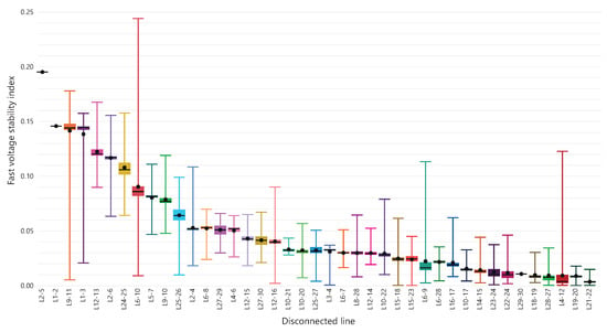
Figure 11.
Thirty-bus-bar system: statistical analysis for every contingency scenario.
Figure 11 presents the information on the minimum, maximum, median, and average FVSI for each contingency scenario. From this graph, and similar to the analysis performed with Algorithm 1 for all contingency scenarios, the most critical ones are those in which line, line, line, or line is disconnected.
Then, continuing with Algorithm 2, after all contingencies are generated in step 3, step 4 applies SVC compensation with values from 5 Mvar to 100 Mvar in steps of 5 Mvar at node i of the weakest power line in every contingency case. Then, the optimal value of compensation and its location are found.
All FVSIs for every connected line when SVC compensation is installed at its optimal location and with the optimal size are represented statistically (due to the massive dataset) in Figure 12. Each scenario has been ordered from the highest to lowest average FVSI for all transmission lines for this graph. This figure shows that the FVSI at line is decreased when compared to its value without compensation.
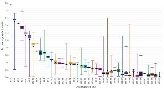
Figure 12.
Thirty-bus-bar system: statistical analysis for every contingency scenario with optimal compensation.
Results Validation
The IEEE 30-bus-bar system has 41 transmission lines; thus, there are 41 contingencies that the algorithm analyzed. For all contingency scenarios, line was selected as the weakest (highest FVSI, not considering PV buses). This paper’s methodology found that a compensation of 45 Mvar in bus bar 9 should be connected to reestablish the system’s stability as close as possible to its values before the contingencies.
From the 41 contingency scenarios, 2 have been selected to be shown and are described below.
- Contingency when the weakest line is disconnected
As can be seen in Figure 11, line is the weakest under all contingency scenarios. As the results of Algorithm 2 indicate, a compensation of 45 Mvar in bus bar 9 should be connected. The FVSI values for every line before the contingency, when line is disconnected, and when the optimal compensation is connected are shown in Figure 13.
Figure 13 shows that the optimal solution reestablished the FVSI values after the contingency occurred to their values before line was disconnected, which proves the algorithm’s performance.
Next, voltages profiles were analyzed. Figure 14 shows the voltage profile of every bus bar before the contingency, when line is disconnected, and when the optimal compensation is connected. This figure shows that the optimal solution reestablished the voltage profile of every bus bar after the contingency occurred to its value before line was disconnected. Once again, the algorithm works as expected.
- Contingency when the transmission line (that contains the bus bar where the SVC is located) is disconnected)
For the IEEE 30-bus bar system, line is the third weakest according to the results of Algorithm 2. Additionally, this scenario is crucial to analyze because the SVC is located in bus bar i from line.
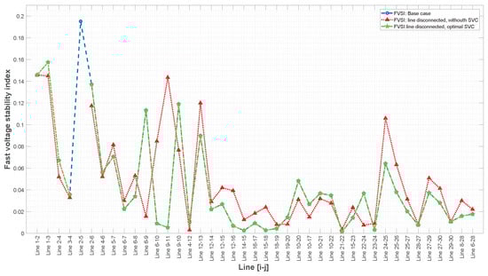
Figure 13.
Second study case: FVSIs before/after contingencies and with SVC compensation, when the weakest line is disconnected.
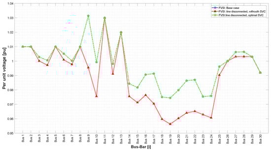
Figure 14.
Second study case: Voltage profiles before/after contingencies and with SVC compensation, when the weakest line is disconnected.
The FVSI values for every line before the contingency, when line is disconnected, and when the optimal compensation is connected are shown in Figure 15. According to these results, even when the disconnected line contains the bus bar where the SVC is located, the algorithm can still reestablish the FVSI values after the contingency occurred to their values before line was disconnected.
Finally, Figure 16 shows the voltage profiles of every bus bar before the contingency, when line is disconnected, and when the optimal compensation is connected.
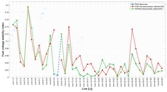
Figure 15.
Second study case: FVSIs before/after contingencies and with SVC compensation, when the line that contains the node for the optimal solution is disconnected.
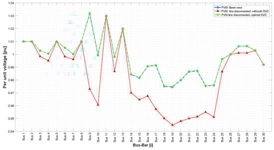
Figure 16.
Second study case: Voltage profiles before/after contingencies and with SVC compensation, when the line that contains the node for the optimal solution is disconnected.
3.3. Case Study: IEEE 118-Bus-Bar System
When applying Algorithm 1 to the IEEE 118-bus-bar system, the FVSI is calculated for every transmission line; this first analysis establishes which power lines are closer to instability by ordering the FVSI from highest to lowest. These data can be seen in Table 3.
Table 3 shows that line has the greatest FVSI and, therefore, is the power line closest to instability. According to Algorithm 2, compensation should be located at node 92; however, node 92 corresponds to a PV bus bar in which, by definition, the voltage profile will not change due to voltage control in this kind of bus bar.
After selecting a transmission line in which node i is not a PV bus, Algorithm 2 selected line, in which compensation will be applied at bus bar 23. After all the contingencies are generated in step 3, step 4 applies SVC compensation with values from 5 Mvar to 100 Mvar in steps of 5 Mvar at node i of the weakest power line in every contingency case. Then, the optimal value of compensation and its location are found. Due to the vast quantity of data, these scenarios are not shown graphically.
After following this procedure, the algorithm’s optimal solution indicated that a compensation of 200 Mvar should be located at bus bar 23.
Table 3.
FVSI of IEEE 118-bus-bar system before contingency scenarios (42 worst lines).
Table 3.
FVSI of IEEE 118-bus-bar system before contingency scenarios (42 worst lines).
| Power Line | FVSI | Power Line | FVSI | Power Line | FVSI | |||
|---|---|---|---|---|---|---|---|---|
| Node i | Node j | Node i | Node j | Node i | Node j | |||
| 92 | 100 | 0.210239 | 94 | 100 | 0.109194 | 8 | 9 | 0.083907 |
| 26 | 30 | 0.201532 | 30 | 17 | 0.107731 | 3 | 5 | 0.083743 |
| 65 | 66 | 0.187142 | 38 | 37 | 0.104339 | 47 | 69 | 0.083263 |
| 62 | 66 | 0.164068 | 100 | 101 | 0.104276 | 80 | 97 | 0.083171 |
| 76 | 77 | 0.155839 | 49 | 69 | 0.103562 | 70 | 74 | 0.08301 |
| 32 | 113 | 0.147749 | 86 | 87 | 0.102972 | 68 | 69 | 0.082493 |
| 9 | 10 | 0.147655 | 110 | 112 | 0.09776 | 80 | 99 | 0.081192 |
| 80 | 96 | 0.145052 | 77 | 80 | 0.097663 | 68 | 81 | 0.077969 |
| 26 | 25 | 0.144684 | 17 | 31 | 0.094327 | 38 | 65 | 0.07716 |
| 49 | 54 | 0.143047 | 19 | 34 | 0.092415 | 3 | 12 | 0.076708 |
| 92 | 94 | 0.129257 | 77 | 82 | 0.090745 | 75 | 77 | 0.07598 |
| 49 | 54 | 0.126068 | 77 | 80 | 0.086265 | 54 | 59 | 0.075348 |
| 23 | 25 | 0.123706 | 55 | 59 | 0.085933 | 62 | 67 | 0.074813 |
| 79 | 80 | 0.113546 | 83 | 84 | 0.085796 | 89 | 92 | 0.07449 |
Results Validation
The IEEE 118-bus-bar system has 186 transmission lines; thus, there are 186 contingencies that the algorithm analyzed. For all the contingency scenarios, line was selected as the weakest (highest FVSI, not considering PV buses). This paper’s methodology found that a compensation of 100 Mvar in bus bar 23 should be connected to reestablish the system’s stability as close as possible to its values before the contingencies.
From the 186 contingency scenarios, the most critical has been selected to be shown and is described below.
- Contingency when the weakest line is disconnected
As can be seen in Table 3, line is the weakest under all contingency scenarios. As the results of Algorithm 2 indicate, a compensation of 100 Mvar in bus bar 23 should be connected. The FVSI values for every line before the contingency, when line is disconnected, and when the optimal compensation is connected are shown in Figure 13.
Figure 17 shows that the optimal solution reestablished the FVSI values after the contingency occurred to their values before line line was disconnected. Due to the many transmission lines, this figure only shows the power lines close to the one disconnected. Additionally, given the massive size of this transmission system, the difference between the scenarios before and after the contingency is barely visible.
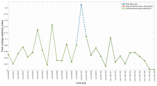
Figure 17.
Third study case: FVSIs before/after contingencies and with SVC compensation.
Next, voltages profiles were analyzed. Figure 18 shows the voltage profile of every bus bar before the contingency, when line is disconnected, and when the optimal compensation is connected. This figure shows that the optimal solution reestablished the voltage profile of every bus bar after the contingency occurred to its values before line was disconnected. Once again, the algorithm works as expected.
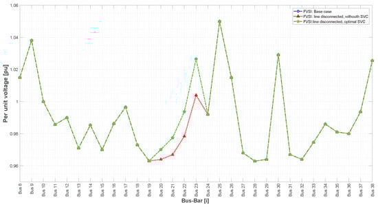
Figure 18.
Third study case: Voltage profiles before/after contingencies and with SVC compensation.
3.4. Results Summary
From the three case studies analyzed in this research, the proposed algorithm found a single bus bar in which SVC compensation is located with the optimal value; consequently, the transmission system will be covered under any contingency scenario, and the fast voltage stability index will not be affected, even when a transmission line is disconnected. Additionally, this solution represents a minimal investment for the system’s operator because the minimum sizing of the SVC is selected, and a single unit of reactive compensation is connected to the system.
Table 4 shows the optimal values of SVC compensation that this research’s algorithm obtained.
Table 4.
Algorithm results for the three case studies.
Finally, it is important to consider the effect of an unexpected increase in the system load (active or reactive). The methodology that this research proposes does not contemplate that scenario; nevertheless, for random increases in loads, it would be necessary to have a variable SVC that will adapt its value in accordance with what this paper’s algorithm proposes and the additional load connected to the system. However, this will be studied in future works.
4. Conclusions
Electrical power systems are subject to unexpected events, for example, the disconnection of a transmission line, which will affect the system’s stability and quality parameters, such as voltage (which will decrease if a transmission line is disconnected). This paper tackles these unexpected events, also named contingencies, in which the system is analyzed under every scenario when one transmission line is disconnected ( contingencies). From the results obtained using this research’s methodology, one of this paper’s contributions is the creation of a procedure that applies to any EPS and finds the optimal location and sizing of an SVC, which will reestablish the system stability (FVSI) and voltage profiles at the lowest possible cost by only installing a single SVC.
Whenever a contingency occurs, all FVSI values for all transmission lines in the EPS are increased; this paper’s most significant contribution consists of finding a single optimal solution for the SVC (location and sizing) that will be able to decrease this index to pre-contingency values for all transmission lines under any contingency scenario; therefore, by only installing a single SVC, the system is guaranteed to operate under normal conditions for all contingencies.
As shown by this paper’s results, for all the case studies under every contingency, it is possible to reduce the average FVSI for the whole transmission system by 20% when compared to scenarios with contingencies but no optimal compensation. Furthermore, when analyzing each scenario individually, the FVSI for every power line returns to its original value when the optimal solution is applied under the contingency, meaning that the system will have a stability index (FVSI) 100% identical to that when no contingencies occurred.
Another crucial aspect of this research is that, under a contingency scenario, the voltage profile of the whole power system will decrease, which affects the power quality; however, the optimal solution found in each case study allows the EPS not only to restore its voltage profiles under the contingency to its values when no contingencies occur (which represents 100% recovery) but also, in some cases, to increase its voltage profiles beyond their original values.
Author Contributions
M.D.J.: conceptualization, methodology, validation, writing—review and editing, data curation, formal analysis. D.F.C.: methodology, validation, writing—review and editing. J.P.M.: writing—review and editing. All authors have read and agreed to the published version of the manuscript.
Funding
This work was supported by Universidad Politécnica Salesiana and GIREI—Smart Grid Research Group.
Data Availability Statement
Not applicable.
Conflicts of Interest
The authors declare no conflict of interest.
Abbreviations
The following abbreviations are used in this manuscript:
| Apparent power at bus bar i | |
| Voltage at sending bus bar i | |
| Voltage at receiving bus bar j | |
| Current at sending bus bar i | |
| Current at receiving bus bar j | |
| Admittance at line | |
| Voltage angle at bus bar i | |
| Voltage angle at bus bar j | |
| Voltage angle difference between nodes i and j | |
| Susceptibility at line | |
| Conductance at line | |
| Active power at node i | |
| Reactive power at node j | |
| Generated active power at node i | |
| Demanded active power at node i | |
| Generated reactive power at node i | |
| Demanded reactive power at node i | |
| Fast voltage stability index at line | |
| Impedance at line | |
| Receiving reactive power from node j to node i | |
| Reactance at line | |
| Electrical parameters of all bus bars in a transmission system | |
| Electrical parameters of generator in an electrical power system | |
| line | Electrical parameters of lines in a transmission system |
| Electrical parameters of loads in a transmission system | |
| Fast voltage stability indices for every line in a transmission system | |
| SVC compensation size to be installed at a bus bar | |
| Optimal bus-bar location for SVC | |
| Optimal sizing of SVC |
References
- Shojaeiyan, S.; Niknam, T.; Nafar, M. A novel bio-inspired stochastic framework to solve energy management problem in hybrid AC-DC microgrids with uncertainty. Int. J. Bio-Inspired Comput. 2021, 18, 165–175. [Google Scholar] [CrossRef]
- Kou, L.; Li, Y.; Zhang, F.; Gong, X.; Hu, Y.; Yuan, Q.; Ke, W. Review on Monitoring, Operation and Maintenance of Smart Offshore Wind Farms. Sensors 2022, 22, 2822. [Google Scholar] [CrossRef] [PubMed]
- Adegoke, S.A.; Sun, Y. Power system optimization approach to mitigate voltage instability issues: A review. Cogent Eng. 2023, 10, 2153416. [Google Scholar] [CrossRef]
- Soyemi, A.; Misra, S.; Oluranti, J.; Ahuja, R. Evaluation of Voltage Stability Indices. In Proceedings of the Information Systems and Management Science, ISMS 2020, Msida, Malta, 15–17 December 2020; Lecture Notes in Networks and Systems. Springer: Cham, Switzerland, 2022; Volume 303, pp. 4–82. [Google Scholar] [CrossRef]
- Carrión, D.; García, E.; Jaramillo, M.; González, J.W. A Novel Methodology for Optimal SVC Location Considering N-1 Contingencies and Reactive Power Flows Reconfiguration. Energies 2021, 14, 6652. [Google Scholar] [CrossRef]
- Panda, S.B.; Mohanty, S. Assessment of Power System Security for Different Bus Systems through FVSI/RFVSI and Fuzzy Logic Approaches. IETE Tech. Rev. 2022, 39, 1485–1500. [Google Scholar] [CrossRef]
- Singh, P.; Singh, J.; Tiwari, R. Performance evaluation and quality analysis of line and node based voltage stability indices for the determination of the voltage instability point. Lect. Notes Electr. Eng. 2020, 607, 367–376. [Google Scholar] [CrossRef]
- Sharma, A.K.; Saxena, A. Prediction of line voltage stability index using supervised learning. J. Electr. Syst. 2017, 13, 696–708. [Google Scholar]
- Mokred, S.; Wang, Y.; Chen, T. Modern voltage stability index for prediction of voltage collapse and estimation of maximum load-ability for weak buses and critical lines identification. Int. J. Electr. Power Energy Syst. 2023, 145, 108596. [Google Scholar] [CrossRef]
- Mokred, S.; Wang, Y.; Chen, T. A novel collapse prediction index for voltage stability analysis and contingency ranking in power systems. Prot. Control Mod. Power Syst. 2023, 8, 7. [Google Scholar] [CrossRef]
- Choudekar, P.; Asija, D.; Ruchira. Prediction of voltage collapse in power system using voltage stability indices. Adv. Intell. Syst. Comput. 2017, 479, 51–58. [Google Scholar] [CrossRef]
- Samuel, I.A.; Katende, J.; Awosope, C.O.A.; Awelewa, A.A. Prediction of voltage collapse in electrical power system networks using a new voltage stability index. Int. J. Appl. Eng. Res. 2017, 12, 190–199. [Google Scholar]
- Samuel, I.; Katende, J.; Awosope, C.; Awelewa, A.; Adekitan, A.; Agbetuyi, F. Power system voltage collapse prediction using a new line stability index (NLSI-1): A case study of the 330-kV Nigerian National Grid. Int. J. Electr. Comput. Eng. 2019, 9, 5125–5133. [Google Scholar] [CrossRef]
- Malathy, P.; Shunmugalatha, A. Enhancement of Maximum Loadability during N-1 and N-2 contingencies with multi type FACTS devices and its optimization using MDE algorithm. In Proceedings of the 2016 IEEE Uttar Pradesh Section International Conference on Electrical, Computer and Electronics Engineering (UPCON), Varanasi, India, 9–11 December 2016; pp. 173–178. [Google Scholar] [CrossRef]
- Jaramillo, M.; Tipán, L.; Muñoz, J. A novel methodology for optimal location of reactive compensation through deep neural networks. Heliyon 2022, 8, e11097. [Google Scholar] [CrossRef] [PubMed]
- Jaramillo, M.; Carrión, D.; Muñoz, J. A Deep Neural Network as a Strategy for Optimal Sizing and Location of Reactive Compensation Considering Power Consumption Uncertainties. Energies 2022, 15, 9367. [Google Scholar] [CrossRef]
- Gupta, S.K.; Mallik, S.K.; Tripathi, J.M.; Sahu, P. Comparison of Voltage Stability Index with Optimal Placement of SSSC Considering Maximum Loadability. In Proceedings of the 2021 International Symposium of Asian Control Association on Intelligent Robotics and Industrial Automation (IRIA), Goa, India, 20–22 September 2021; pp. 101–106. [Google Scholar] [CrossRef]
- Zellagui, M.; Lasmari, A.; Settoul, S.; El-Bayeh, C.Z.; Chenni, R.; Belbachir, N. Arithmetic Optimization Algorithm for Optimal Installation of DSTATCOM into Distribution System based on Various Voltage Stability Indices. In Proceedings of the 2021 9th International Conference on Modern Power Systems (MPS), Cluj-Napoca, Romania, 16–17 June 2021. [Google Scholar] [CrossRef]
- Venu, Y.; Gnanendar, R. Optimization of Shunt Compensation for Voltage Stability Improvement Using PSO. In Advances in Automation, Signal Processing, Instrumentation, and Control, Proceedings of the i-CASIC 2020, Vellore, India, 27–28 February 2020; Komanapalli, V.L.N., Sivakumaran, N., Hampannavar, S., Eds.; Lecture Notes in Electrical Engineering; Springer: Singapore, 2021; pp. 2929–2940. [Google Scholar]
- Shiferaw, Y.; Padma, K. Enhancement of Power Flow with Reduction of Power Loss Through Proper Placement of FACTS Devices Based on Voltage Stability Index. In Proceedings of the Advances of Science and Technology, Bahir Dar, Ethiopia, 2–4 August 2019; Habtu, N.G., Ayele, D.W., Fanta, S.W., Admasu, B.T., Bitew, M.A., Eds.; Springer International Publishing: Cham, Switzerland, 2020; pp. 355–365. [Google Scholar]
- Jirjees, M.A.; Al-Nimma, D.A.; Al-Hafidh, M.S.M. Voltage Stability Enhancement based on Voltage Stability Indices Using FACTS Controllers. In Proceedings of the 2018 International Conference on Engineering Technology and their Applications (IICETA), Al-Najaf, Iraq, 8–9 May 2018; pp. 141–145. [Google Scholar] [CrossRef]
- Meena, G.; Verma, K.; Mathur, A. FVSI Based Meta-heuristic Algorithm for Optimal Load Shedding to Improve Voltage Stability. In Proceedings of the 2022 IEEE 10th Power India International Conference (PIICON), New Delhi, India, 25–27 November 2022. [Google Scholar] [CrossRef]
- Pacis, M.C.; Antonio, I.J.M.; Banaga, I.J.T. Under Voltage Load Shedding Algorithm using Fast Voltage Stability Index (FVSI) and Line Stability Index (LSI). In Proceedings of the 2021 IEEE 13th International Conference on Humanoid, Nanotechnology, Information Technology, Communication and Control, Environment, and Management (HNICEM), Manila, Philippines, 28–30 November 2021. [Google Scholar] [CrossRef]
- Salama, H.S.; Vokony, I. Voltage stability indices—A comparison and a review. Comput. Electr. Eng. 2022, 98, 107743. [Google Scholar] [CrossRef]
- Li, Y.; Zhang, M.; Chen, C. A Deep-Learning intelligent system incorporating data augmentation for Short-Term voltage stability assessment of power systems. Appl. Energy 2022, 308, 118347. [Google Scholar] [CrossRef]
- Heidari Yazdi, S.S.; Rahimi, T.; Khadem Haghighian, S.; Gharehpetian, G.B.; Bagheri, M. Over-Voltage Regulation of Distribution Networks by Coordinated Operation of PV Inverters and Demand Side Management Program. Front. Energy Res. 2022, 10, 920654. [Google Scholar] [CrossRef]
- Grisales-Noreña, L.; Morales-Duran, J.; Velez-Garcia, S.; Montoya, O.D.; Gil-González, W. Power flow methods used in AC distribution networks: An analysis of convergence and processing times in radial and meshed grid configurations. Results Eng. 2023, 17, 100915. [Google Scholar] [CrossRef]
- Musirin, I.; Abdul Rahman, T.K. Novel fast voltage stability index (FVSI) for voltage stability analysis in power transmission system. In Proceedings of the 2002 Student Conference on Research and Development: Globalizing Research and Development in Electrical and Electronics Engineering, SCOReD 2002—Proceedings, Shah Alam, Malaysia, 17 July 2002; pp. 265–268. [Google Scholar] [CrossRef]
Disclaimer/Publisher’s Note: The statements, opinions and data contained in all publications are solely those of the individual author(s) and contributor(s) and not of MDPI and/or the editor(s). MDPI and/or the editor(s) disclaim responsibility for any injury to people or property resulting from any ideas, methods, instructions or products referred to in the content. |
© 2023 by the authors. Licensee MDPI, Basel, Switzerland. This article is an open access article distributed under the terms and conditions of the Creative Commons Attribution (CC BY) license (https://creativecommons.org/licenses/by/4.0/).