Fatigue Life Convergence of Offshore Wind Turbine Support Structure According to Wind Measurement Period

Abstract

This paper investigated the fatigue life of offshore wind turbine (OWT) support structures. For this purpose, a 3 MW-capacity typical wind turbine is investigated using time-domain finite element simulations. In numerical simulations, different stochastic wind models corresponding to different accumulation periods are applied. Then, the stress-based fatigue life is estimated following the rain-flow counting algorithm and Palmgren-Miner linearly cumulative damage rule. The study also addresses the joint distribution of loads at the site of interest. Generally, the study emphasizes the significance of the long-term distribution of the applied environment loads and its influence on the fatigue life of OWT’s substructures. The results imply that the wind measurement period is directly linked to the fatigue life of offshore wind turbine support structures. Accordingly, its fatigue life is significantly reduced at the 25-year accumulative period of wind. Therefore, this study recommends that a sufficient number of accumulative periods of wind and other environmental loads should be considered appropriately.

1. Introduction

Compared to onshore wind turbines, offshore wind farms are more exposed to extreme environmental conditions, including extreme wind loads, wave loads, and natural disasters such as typhoons, tornadoes, etc. And the supporting structures of offshore wind turbines are considered the main components subjected to these complex loads. The intensity, as well as the characteristics of these types of loads, are different depending on the specific location. Therefore, an accurate and comprehensive assessment of possible hazards allows optimal design and balance between safety and cost. Because of the harsh marine conditions, offshore structures often suffer unpredicted and complex vibrations. These periodic vibrations caused by the environmental load weaken the material at the critical spots leading to damage to the structure of the material and eventual failure. This phenomenon is so-called fatigue. Fatigue caused by environmental loads can lead to severe damage to the OWT-suction bucket foundations. In particular, this fatigue damage often develops gradually and is difficult to observe. Over the past decades, countless studies have been carried out concerning potential factors which will cause severe fatigue damage. Passon et al. [1] proposed a new wind-wave correlation method based on the establishment of damaged contour lines for the fatigue design at different locations within the offshore wind turbine. Sun et al. [2] used a three-dimensional pendulum-tuned mass damper to mitigate the fatigue damage of offshore wind turbines under real wind and wave conditions. Nejad et al. [3] proposed a method to calculate the long-term fatigue damage based on the S-N approach by considering all short-term damages and the long-term wind speed distribution. Velarde and his colleagues [4] studied the sensitivity of waves on the fatigue reliability of a large monopile supporting a 10 MW offshore wind turbine.

The designed service life of the OWTs is at least 20 years [5,6]. And among the potential hazards, wind load is considered the primary threat to affect the behavior of OWT structures [7,8]. Numerous studies have been in the literature regarding the impact of wind load on structural fatigue. Li et al. [9] found that the fatigue life of the monopile foundation decreased when wind loads were calculated from non-Gaussian wind fields. In his study, a comparison of the effects of Gaussian and non-Gaussian wind fields on wind turbine structure behavior was also performed. Wenbin and his colleague [8] evaluated the fatigue damage of offshore wind turbines under several combinations of environmental loads of wind and waves and found that fatigue damage was caused mainly by wind loads. It agreed well with the study by Oest et al. [10], who also concluded that wave loading does not significantly contribute to accumulative fatigue damage. Wang et al. [11] examined the influence of actual wind loading direction on deterministic fatigue damage.

In previous studies, many incomprehensive efforts have been made to investigate the effect of wind parameters on fatigue lifetime, such as wind speed, wind direction, wind probability distribution model, combination with other environmental loads, etc. In this study, an attempt was made to investigate the influence of another aspect of environmental wind load, the wind accumulative period, on the OWT substructure fatigue lifetime. For convenience, stochastic wind models, i.e., the probability distribution of wind, are usually estimated based on short-term observational data. This approach can lead to an underestimation of fatigue damage. Therefore, this study proposed establishing a wind probabilistic model based on data measured over 1 to 25 years. A joint probabilistic model in terms of wind speed, significant wave height, and peak period was then established, corresponding to the measurement period. The rain-flow counting algorithm and Palmgren-Miner linearly cumulative damage rule were used to estimate cumulative damage. Finally, the fatigue life of the OWT support structures according to the wind measurement period was obtained.

2. Joint Probabilistic Model of Environmental Loads

In previous fatigue analyses, the correlation of the environmental loads, i.e., wind and waves, was not adequately considered; these loads were assumed to be discrete variables instead. In reference to IEC 61400-3 [12], the joint probability model in terms of mean wind speed ($V$), significant wave height ($H_s$), and peak period ($T_p$) was established in the current paper.

2.1. Distribution of Mean Wind Speed (V)

In the current paper, the hind-cast simulation data in Korea over 25 years was used [13]. In reference [14], for wind speed calculation, the N160 Gaussian grid used in the ECMWF wind data model was applied to the entire Korean sea. The grid spacing differed in the latitude direction, and the grid number in the longitude direction differed depending on the latitude. Wind data at points not on the grid were calculated by interpolation. Using ERA-Interim as initial and boundary conditions, a high-resolution wind hindcast for 25 years around Korea was then established. The report provides a reference dataset for research related to the design, performance evaluation, and risk analysis of marine structures. Wind data used in the study are estimated at 10 m above mean sea level. Since the wind loads were applied at the top of the tower, the following power law can be used.

$$u_z=u_{hub}{\left(\frac{z}{z_{hub}}\right)}^{\alpha }$$

(1)

Although previous studies [13,15,16,17] have proved that the two-parameter Weibull distribution is suitable for simulating the wind speed distribution, the measured wind speed data at the survey site in the current research fit better with the Generalized Pareto (GP) distribution. This distribution depends on three parameters: location ($\mu$), scale ($\sigma$), and shape ($\xi$). The probability density function (PDF) is shown in Equation (2).

$$f_V\left(u\right)=\left(\frac{1}{\sigma }\right){\left(1+\xi \frac{\left(u-\mu \right)}{\sigma }\right)}^{-1-\frac{1}{\xi }}$$

(2)

Figure 1a shows the comparison of PDFs. While the data was represented in the form of a histogram, several distributions, such as Normal, Weibull, Lognormal, and Generalized Pareto (GP), were described by a variety of lines. It can be seen that GP distribution shows better performance compared to others. The results of a goodness of fit test shown in Figure 1b indicates a similar conclusion.

2.2. Conditional Distribution of $H_s$ Given $V$

Previous studies [13,15] show that conditional probability distributions $H_s$ given $V$ can be modeled by a two-parameter Weibull distribution, as follows:

$$f_{H_s│V}\left(h│u\right)=\frac{k_h}{{\sigma }_h}{\left(\frac{h}{{\sigma }_h}\right)}^{k_h{}^{-1}}exp{\left(-\frac{h}{{\sigma }_h}\right)}^{k_h}$$

(3)

where $k_h$ and ${\sigma }_h$ are the shape and scale parameters that can be calculated by Equation (4), respectively. The parameters $a_k$, $b_k$, $c_k$, $a_{\sigma }$ and $b_{\sigma }$ here are the parameters obtained from curve fitting.

$$\begin{array}{c}{k}_h=a_k+b_k\ast u^{c_k}\\ {\sigma }_h=a_{\sigma }+b_{\sigma }\ast u\end{array}$$

(4)

2.3. Conditional Distribution $T_p$ of Given $V$ and $H_s$

By giving mean wind speed ($V$) and the significant wave height ($H_s$) with a bin size of 1 m/s and 0.1 m, respectively, the peak period ($T_p$) data are recalculated, and a lognormal distribution was used to describe the conditional distribution of $T_p$ given $V$ and $H_s$, as shown in Equation (5). ${\mu }_{\ln \left(T_p\right)}$ and ${\sigma }_{\ln \left(T_p\right)}$, which are the mean and standard deviation of the lognormal distribution, respectively, can be obtained by Equation (6).

$$f_{T_p│V,H_s}\left(t│u,h\right)=\frac{1}{\sqrt{2}{\sigma }_{\ln {\left(T_p\right)}^t}}exp\left[-\frac{1}{2}{\left(\frac{\ln \left(t\right)-{\mu }_{\ln \left(T_p\right)}}{{\sigma }_{\ln \left(T_p\right)}}\right)}^2\right]$$

(5)

$$\begin{array}{c}{\mu }_{\ln \left(T_p\right)}=\ln \left[\raisebox{1ex}{${\mu }_{T_p}$}\!\left/ \!\raisebox{-1ex}{$\sqrt{1+{\left({\sigma }_{T_p}/{\mu }_{T_p}\right)}^2}$}\right.\right]\\ {\sigma }_{\ln \left(T_p\right)}=\ln \left[{\left({\sigma }_{T_p}/{\mu }_{T_p}\right)}^2+1\right]\end{array}$$

(6)

where ${\mu }_{T_p}$ and ${\sigma }_{T_p}$ are the mean and standard deviation of $T_p$ distribution in each wind-wave class, respectively. These parameters were obtained by Equation (7).

Table 1. Probabilistic model parameters.

Distribution	Parameter	Value
Distribution of $V$	$\mu$	2.351
	$\sigma$	3.521
	$\xi$	−0.154
Distribution of $H_s$ given $V$	$a_k$	1.918
	$b_k$	7.989
	$c_k$	2.107
	$a_{\sigma }$	−0.452
	$b_{\sigma }$	0.273
Distribution of $T_p$ given $V$ and $H_s$	$a_{\mu }$	−0.138
	$b_{\mu }$	−0.069
	$c_{\mu }$	0.589
	$d_{\mu }$	1.045
	$e_{\mu }$	1.154
	$f_{\mu }$	0.146
	$g_{\mu }$	0.142
	$h_{\mu }$	0.581
	$a_{{\sigma }_T}$	33.161
	$b_{{\sigma }_T}$	−32.971
	$c_{{\sigma }_T}$	0.001

summarizes the parameters for the distribution of $V$, the conditional distribution of $H_s$ given $V$ and the conditional distribution of $T_p$ given both $V$ and $H_s$.

$$\begin{array}{c}{\mu }_{T_p}=\left(a_{\mu }+b_{\mu }·H_s^{c_{\mu }}\right)·\left\{d_{\mu }-e_{\mu }·\left[\raisebox{1ex}{$U_w-\left(f_{\mu }+g_{\mu }·H_s^{h_{\mu }}\right)$}\!\left/ \!\raisebox{-1ex}{$f_{\mu }+g_{\mu }·H_s^{h_{\mu }}$}\right.\right]\right\}\\ {\sigma }_{T_p}={\mu }_{T_p}\left[a_{{\sigma }_T}+b_{{\sigma }_T}·\exp \left(c_{{\sigma }_T}·H_s\right)\right]\end{array}$$

(7)

3. Estimation of Environmental Loads

In this study, besides the probabilistic fatigue analysis, stress-based fatigue life was also evaluated by the deterministic approach in which the input loads, i.e., wind and waves, were obtained by a deterministic model. As discussed, the wind speed ($V$), significant wave height ($H_s$), and peak wave periods ($T_p$) were used to set the conditions of the environment, which were then applied as the input conditions. Simulation in the time domain was proved to be the popular practice. Unfortunately, this method takes a lot of time in terms of computation. Therefore, this study first applies loading input and starts to analyze the dynamic response of the structure in the frequency domain. After obtaining a stress spectrum corresponding to structural response under the impact of a specific combination load, the transfer function will be used to transform it into the time domain.

3.1. Estimation of Wind Load

Gh-Blade [18] is the open source adopted to calculate the thrust of the wind in this study. Accordingly, the wind field was generated using the Kaimal model by giving parameters such as mean wind speed, turbulence intensity, etc., as shown in Equation (8). The time series of thrust were then obtained and used as the input wind loads in finite element (FE) models. The time series of wind and other environmental loads, i.e., wave loads, were calculated with an interval of 0.1 s to be suitable for the time step of the finite element simulation. 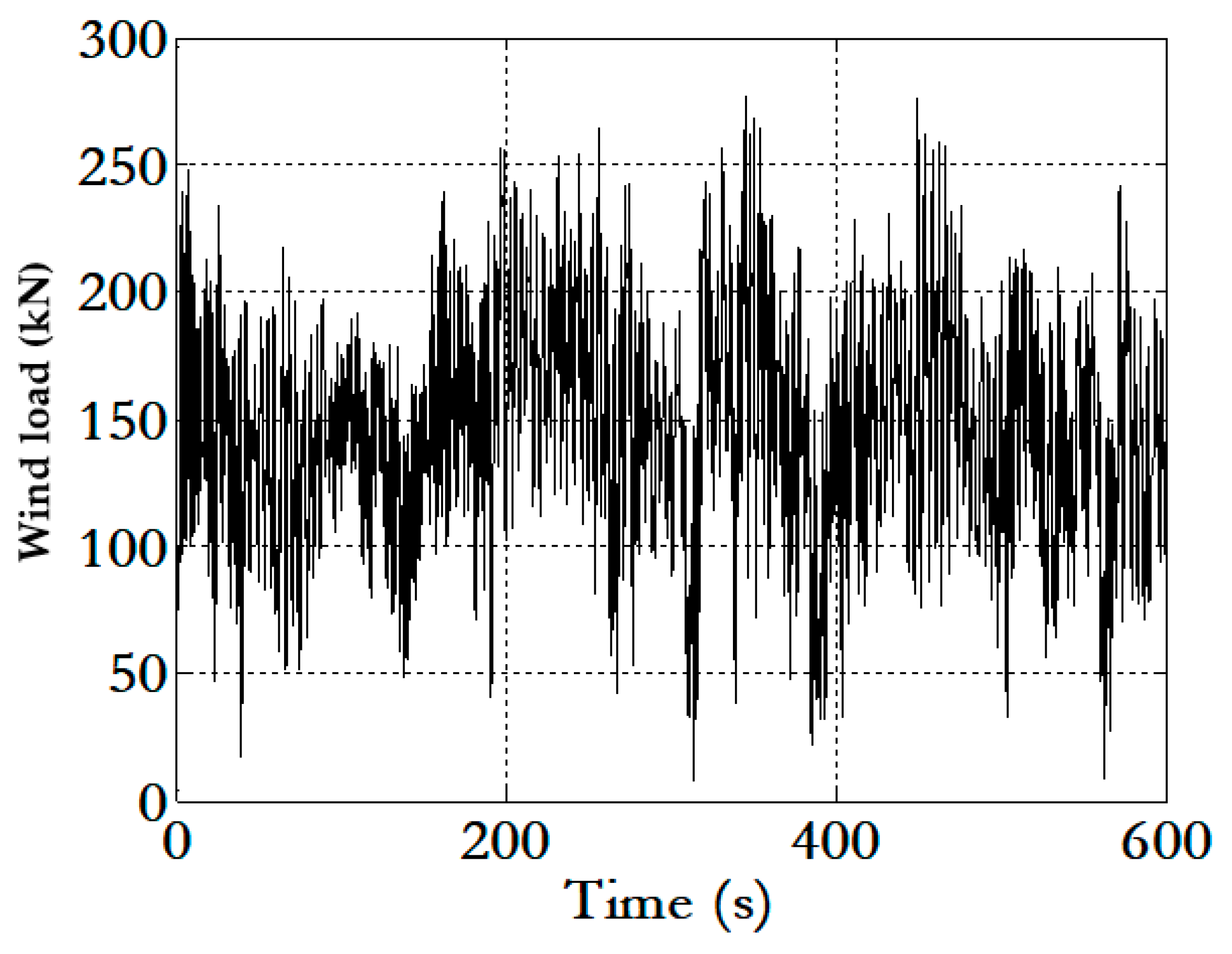Figure 2 illustrates the wind thrust at the hub height in the case of a wind speed of 10 m/s and the turbulence intensity (Iref) of 0.12, corresponding to the rated wind speed of a 3 MW OWT.

$$S\left(n\right)=\frac{4{\sigma }_u^2{n}_u/n}{{\left(1+6n_u\right)}^{5/3}}$$

(8)

where $n$ is the frequency of variation, ${\sigma }_u$ is the standard deviation of wind speed variation, $n_u=n{L}_1/u$ is a non-dimensional frequency parameter, $L_1$ is defined by the turbulence scale parameter, and $u$ is the mean wind speed.

3.2. Peak Wave Period

Because the wave period mentioned in the data is the significant wave period $T_s$, the following equation by Goda [19] should be used to estimate the peak wave period $T_p$. Here, $\gamma$ is a peak enhancement factor.

$$\begin{array}{c}{T}_p\cong T_s·\left[1-0.132·{\left(\gamma +0.2\right)}^{-0.559}\right]\\ \gamma =1 ~ 7 \left(mean of 3.3\right)\end{array}$$

(9)

3.3. Estimation of Wave Load

Figure 3 illustrates the applicability ranges of various waves in the design of the offshore structure [20]. The calculation of wave loads on the cylindrical members of the OWT studied in this paper was adopted from Morrison’s equation. Accordingly, the horizontal forced $dF$ acting on a strip of length $dz$ can be written as:

$$dF=C_D\frac{1}{2}{\rho }_{w}D{v}_x\left|v_x\right|dz+C_I{\rho }_w\frac{\pi }{4}{D}^2{a}_{x}dz$$

(10)

where $C_D$ and $C_I$ are coefficients represent the viscous and inertia terms, ${\rho }_w$ denoted the water density, and $D$ is the diameter of the cylindrical structure. $v_x$ and $a_x$ are the wave-induced horizontal velocity and acceleration of fluid particles.

In this study, Bretschneider’s wave spectrum was used to generate wave time histories.

$$S\left(f\right)=0.257H_s^2{T}_s^{-4}{f}^{-5}exp\left[-1.03{\left(T_{s}f\right)}^{-4}\right]$$

(11)

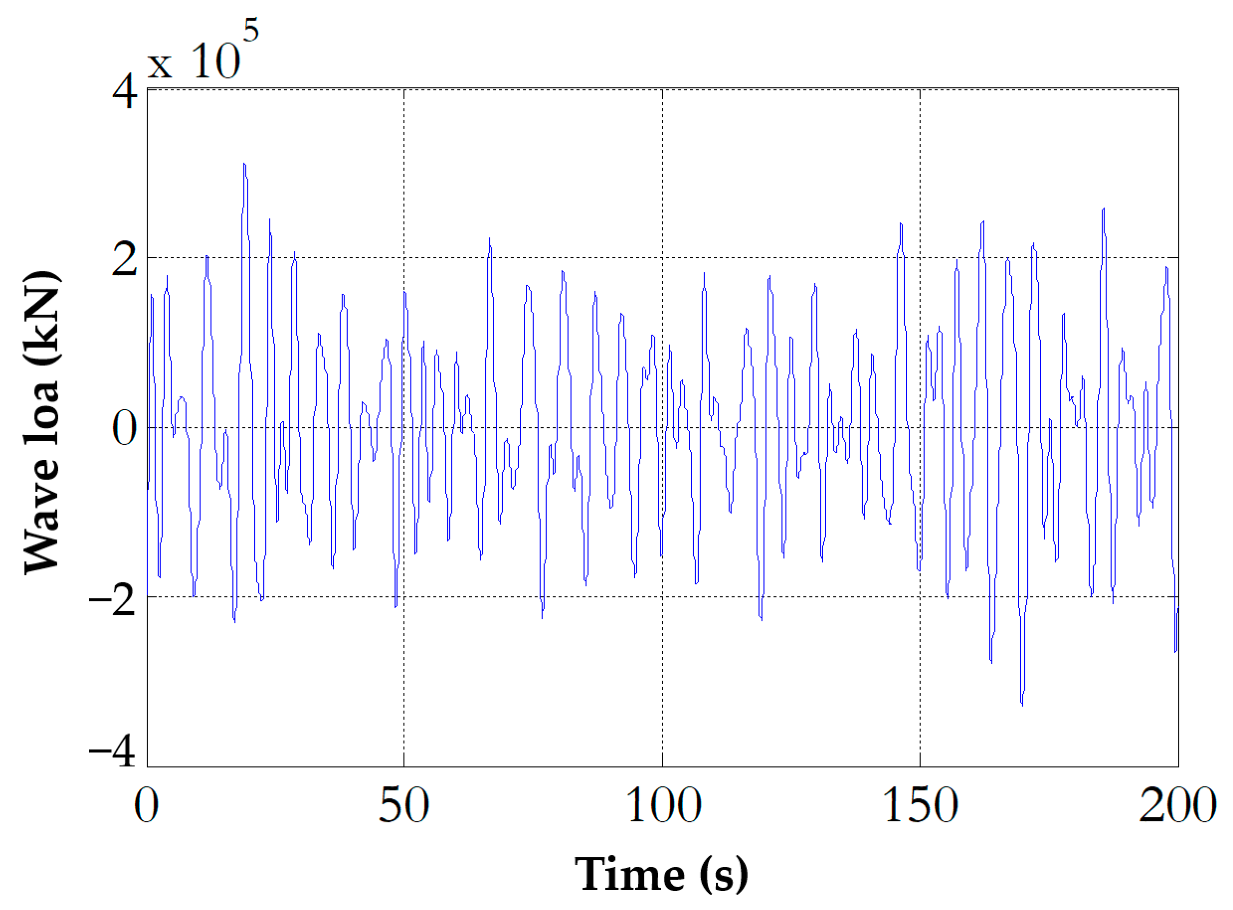
where $H_s$ and $T_s$ are the significant wave height and period, $f=1/T_s$. Figure 4 illustrates the wave load at sea level in the case of $H_s$ and $T_s$ of 2.74 m and 6.23 s, respectively.

4. Support Structure Used for Analysis

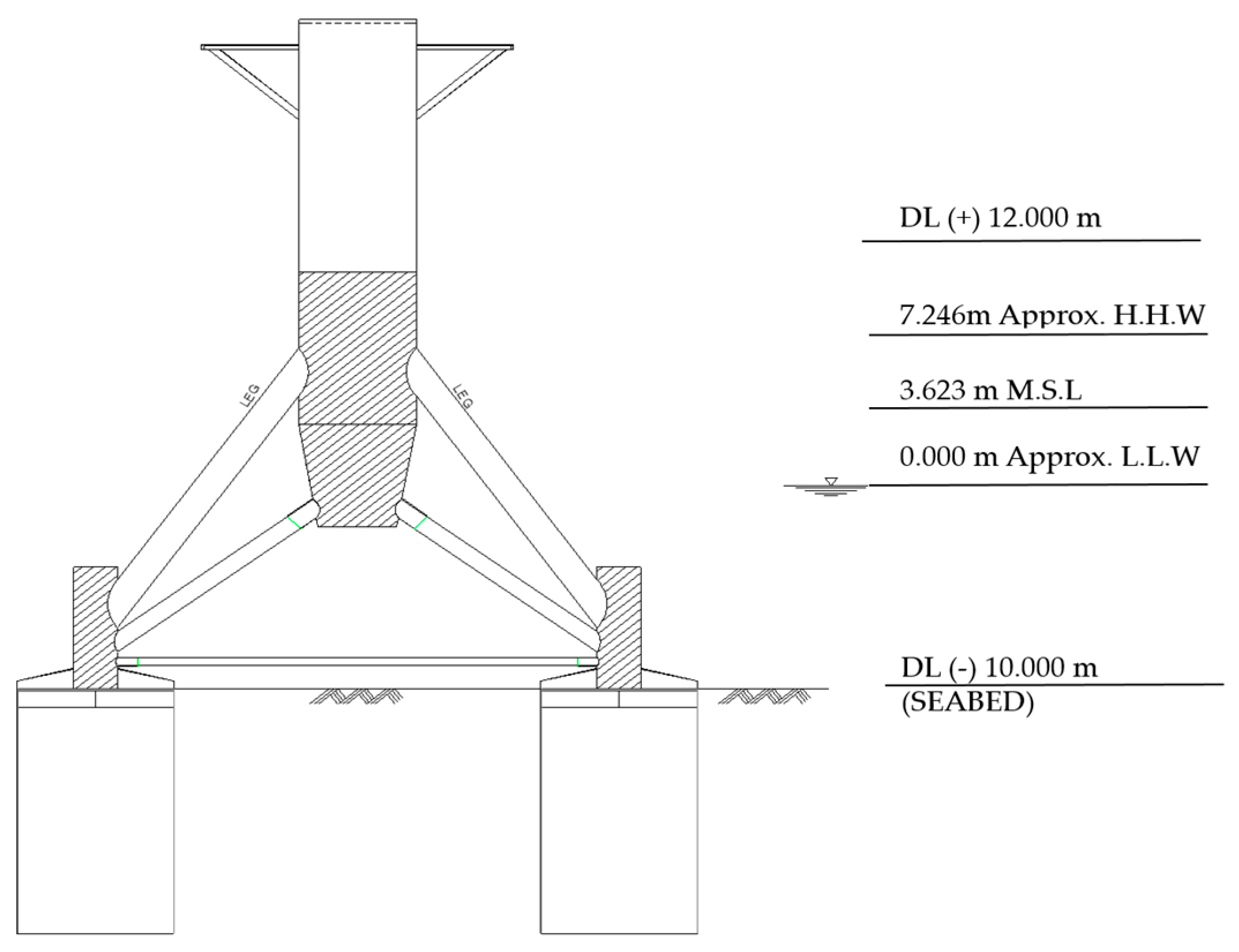
In the current research, a 3 MW-capacity OWT was used as a case study. Its main parameters are described in

Table 2. 3 MW-capacity wind turbine main parameters.

Parameter	Value
Rating (MW)	3
Hub height (m)	80.0259
Number of blades	3
Cut-in, rate, cut-out wind speed (m/s)	3, 10, 25
Rotor mass (ton)	58
Nacelle mass (ton)	128
Tower mass (ton)	358
Mean sea level (m)	13.623
Density of steel (tower and substructure) (kg/m3)	7850
Young’s modulus of steel (GPa)	210
Poisson’s ratio of steel	0.3

and Figure 5. The suction bucket foundation has been demonstrated to be a potential foundation for OWTs and has been investigated in numerous previous studies [21,22,23]. In this study, the support structure was a tripod suction bucket. To account for the effect of the soil on the behavior of the structure, the soil medium was also modeled, and the soil parameters are listed in

Table 3. Soil parameters.

Soil Layer	Depth	Unit Weight	Modulus of Deformation	Internal Friction Angle	Undrained Shear Strength	Poisson’s Ratio
Upper sand	0.0~2.5	1.9	21,000	23.5	-	0.491
Upper clay	2.5~8.3	1.8	25,500	-	7.08	0.491
Lower sand	8.3~10.7	1.9	41,700	35.3	-	0.487
Lower clay	10.7~15.7	1.8	43,000	-	7.08	0.488
Weathered soil	15.7~21.2	1.8	74,600	30	-	0.482
Weathered rock	21.2~	2.0	76,000	32	-	0.450

. The elastic-perfectly plastic Mohr-Coulomb constitutive model was used to describe the complex behavior of the soil. The surface-to-surface master/slave contact pair, one of the features of Abaqus, was used to model the interaction between the bucket skirt and the surrounding soil. In the numerical model, the hub–blade–nacelle assembly, simplified as a centralized mass, was connected to the top of the tower with coupled constrain. C3D8R elements were used for modeling the soil, and beam elements were used for the tower. The tower’s diameter varied in height from 4.5 m to 3.07 m, and the average thickness of the tower was approximately 0.023 m. The suction bucket had a diameter, length, and thickness of 6 m, 12 m, and 0.019 m, respectively. It was modeled using the shell element. The total number of elements in the whole computational domain was about 50,000, and the total degree of freedom was about 150,000. The element size of the tower and substructure was about 0.8 m and 0.5 mm, respectively, and the minimum element size of the seabed foundation surrounding the suction bucket and suction bucket was about 0.5 m. The finite element model is shown in Figure 6.

5. Fatigue Analysis

In this study, both deterministic and probabilistic methods were used to investigate the fatigue life of OWT substructures. In the probabilistic method, to investigate the fatigue life convergence of OWT substructures according to the wind measurement period, the different distribution models of wind speed were estimated for the different accumulation periods of data (from 1 to 25 years). Given these wind speed distributions, the conditional distribution of significant wave height and peak period were also calculated accordingly, as presented in Section 2. Based on these distributions and the range of possible values for each uncertain parameter (wind speed, significant wave height, and period), a set of sample points was selected using the saturated design method. For each set of the sample point, a simulation of the structure under the given wind and wave loading conditions was performed to determine the fatigue life. The results from all of the simulations were collected, and the distribution of fatigue life was then estimated. For model comparison and validation, the hourly wind speed data of 6 days was used as input data. The fatigue life was then calculated by both deterministic and probabilistic methods.

The numerical operation flow is shown in Figure 7. It shows the probabilistic fatigue life analysis procedure where the block denoted by “joint probability model” is a process of probabilistically extracting environmental loads. Skipping the joint probability model block and going directly to “environmental load calculation” block results in a deterministic fatigue life analysis procedure. In the probabilistic calculation of fatigue life, the iteration loop is executed until convergence, but the loop is not iterated in the deterministic approach.

5.1. Rain-Flow Counting (RFC) Method

The stress histories obtained at the most vulnerable point of the OWT substructure under environmental loads are complex and impossible to apply in the fatigue failure analysis without conversion. Through several counting methods, these stress-time histories can be expressed as the relationship between stress range level and its number of cycles. There are several common cycle counting methods reported in the literature, and the RFC method is considered to be the most accurate, as demonstrated by the research of Frendahl and Rychlik [24]. The most significant advantage of this method is that no un-countable small amplitudes are omitted in the calculation process; the fatigue analysis results are, therefore, more reliable. Another strong point of the RFC method is that Palmgren-Miner linearly cumulative damage rule can be easily applied to calculate the fatigue damage in the following steps. The stress time histories are then converted in terms of stress amplitude levels and the accumulated number of cycles.

5.2. Goodman Equation and the Determination of S-N Curve

In this study, the Goodman equation [25] was applied to calculate the equivalent stress amplitude by using the stress range level (${\sigma }_a$) and the mean stress (${\sigma }_u$) obtained in the previous step (rain-flow counting).

$$\frac{{\sigma }_a}{{\sigma }_e}+\frac{{\sigma }_m}{{\sigma }_u}=1\Rightarrow {\sigma }_e=\frac{{\sigma }_u{\sigma }_a}{{\sigma }_u-{\sigma }_m}$$

(12)

where ${\sigma }_e$ is equivalent to stress amplitude and ${\sigma }_m$ is the tensile strength limit of the material.

As mentioned earlier, the stress range level and corresponding cycle number are counted by the RFC approach, and the S-N curve is used to predict fatigue life. In the current study, the equation recommended by DNV [5] is referred to estimate the fatigue life.

$$lo{g}_{10}N=lo{g}_{10}\overline{a}-mlo{g}_{10}\left[{\sigma }_e{\left(\frac{t_{ref}}{t}\right)}^k\right]$$

(13)

where $t_{ref}$ and $t$ are the reference (0.016 m) and component thickness. Parameter k denotes the index parameter. $N$ is the number of stress cycles to failure corresponding to the equivalent stress amplitude (${\sigma }_e$), $\overline{a}$ and $m$ define the intercept and negative inverse slope of the S-N curve, respectively. With reference to [5], for welded tubular joints, these parameter values are chosen and shown in

Table 4. Parameters of S-N curve.

Case	$\mathit{l}\mathit{o}{\mathit{g}}_{10}\overline{\mathit{a}}$	$\mathit{m}$
$N\le {10}^7$	12.48	3
$N>{10}^7$	16.13	5

.

5.3. Cumulative Damage Law

Cumulative fatigue damage is calculated based on Miner’s law.

$$D={\displaystyle \sum }_{i=1}^n\frac{n_i}{N_i}$$

(14)

where, $n$, $n_i$ and $N_i$ are the total number of stress cycles, the number of stress cycles in the $i$th stress amplitude, and the number of cycles to fatigue failure corresponds to the equivalent stress amplitude $i$th. Fatigue damage is examined at maximum stress (hot spot). The hot spot in the substructure for OWT in the current study was evaluated and found to be approximately at the mean sea level, as indicated in Figure 8. The fatigue life of the structure was estimated based on the cumulative fatigue damage of this hot spot. By applying different input loads corresponding to different accumulation periods, the correlation between the fatigue life and the environmental load accumulation period could be obtained.

5.4. Verification of Proposed Method

In this section, to confirm the reliability of the proposed approach, an analysis was performed. Input loads were estimated from 6-day measurement data. For comparison, the fatigue life was calculated using deterministic and probabilistic methods. The PDF of wind speed was estimated from the hourly wind speed data recorded in 6 days. The corresponding conditional PDFs of significant wave height and peak period were also calculated using this PDF of wind speed. In the deterministic method, the mean value of these PDFs was used to calculate the load input.

The fatigue life result obtained by the probabilistic method is shown in Figure 9a. Several distributions were performed, and the distribution of fatigue life, in this case, was found to be suitable for log-normal distribution. The K-S (Kolmogorov-Smirnov) test results shown in Figure 9b and

Table 5. Kolmogorov-Smirnov test results.

Distribution	$\mathbf{Critical}\mathbf{Value}\left({\mathit{D}}_{\mathit{n}}^{ \mathit{\alpha }}\right)$	$\mathbf{Maximum}\mathbf{Difference}\left({\mathit{D}}_{\mathit{n}}\right)$	p-Value
Normal	0.0569	0.0283	0.7469
Log-normal		0.0171	0.9958
GEV		0.0204	0.9699
Weibull		0.0785	0.0018

confirm the above conclusion. The log-normal distribution provided the largest p-value, implying it performs better than other distributions.

The predicted fatigue life of the OWT substructure by both methods is presented in

Table 6. Fatigue life comparison.

Method	Fatigue Life [year]	Relative Error for Fatigue Life [%]	Distribution	Coefficient of Variation (COV)
Deterministic	32.720 (Constant)	−6.19	-	-
Probabilistic	34.745 (Mean)		Log-normal	0.0614

. It is evident from Table 6 that the fatigue life value obtained using the deterministic method was approximately 6.19% smaller than the probabilistic method. In the literature, the deterministic method has been evaluated as a safer structural risk assessment method. However, it is not cost-effective. Therefore, depending on the target level of design, the balance of safety, and cost-effectiveness, the appropriate method can be selected.

5.5. Fatigue Life According to Accumulation Period of Wind Data

As discussed in Section 2.1, to establish the wind speed distribution at a survey site, the three-parameters Generalized Pareto (GP) distribution was used. In the current study, the different models of wind speed distribution were obtained by considering the different numbers of accumulation times over 1 to 25 years. The interval is one year. Corresponding to each input load, the cumulative fatigue damage at the most vulnerable point of the OWT substructure was calculated, and the corresponding fatigue life was also calculated based on this cumulative fatigue damage. Finally, the relationship between fatigue life and wind load accumulation time was examined. The results are shown in Figure 10.

From Figure 10, it is evident that the value of fatigue life fluctuates slightly when the input load is estimated based on data accumulated over 1 to 23 years, and into a significant reduction when the data accumulation period above 23 years is considered. It indicates that the wind measurement period has a definite influence on the fatigue life of the OWT substructure. Specifically, corresponding to the wind accumulation period of 1–23 years, fatigue life ranges from 27.91 to 28.83 years, and the average value is approximately 28.42 years. However, with a wind accumulation period of 24 years, the fatigue life is 24.8 years, a decrease of 12.7%. This value becomes 24.47 years (13.9% decrease) when 25 years of wind is used. This decrease in fatigue life is caused by a rapid increase in wind speed between 24 and 25 years. Therefore, it is necessary to predict fatigue life using the wind speed for a long period rather than the wind speed of a specific period with high variability. It can be said that the previous application of short-term distribution of environmental loads in the probabilistic fatigue analysis can lead to the underestimation of fatigue damage. The long-term distribution of environmental loads should be appropriately applied.

6. Conclusions

Fatigue life convergence of the OWT substructure according to a wind measurement period was investigated in this study. An FE model of a 3 MW case study OWT was used. Fatigue analysis was conducted regarding stress time history at the most vulnerable point of the OWT substructure. The stress cycles in time history were then counted by the RFC method, the S–N curve was used to predict the fatigue life, and the Palmgren-Miner linearly cumulative damage rule was used to estimate the total fatigue damage. Additionally, the fatigue life was calculated by both the deterministic and probabilistic methods. It was found that the determination method can lead to an underestimation of fatigue damage. The probabilistic fatigue analysis was conducted using the different distribution models of wind speed with respect to different accumulation periods of data (from 1 to 25 years). The joint distribution in terms of mean wind speed ($V$), significant wave height ($H_s$), and peak period ($T_p$) was also established during the calculation. Finally, the value of fatigue life varied depending on the used wind accumulation period. Specifically, the average fatigue life value was approximately 28.42 years for the 1 to 23-year wind measurement period. With the 25-year wind measurement period, fatigue life decreased significantly, approximately 13.9%, to 24.47 years. Thus, this study recommends the effect of the environmental load measurement period on the fatigue life of the OWT substructure should be considered appropriately.

In this paper, only uncertainties of the external loads were considered. The consideration of the uncertainties of the material properties and their effect on the fatigue behavior of structures is suggested for further study. Furthermore, the S-N curves from DNV for offshore steels that have no distinction among different materials in offshore codes are also a limitation of this work. Further works related to the S-N approach to obtain the fatigue damage for different materials of OWT substructure would be an interesting topic.

References

- Passon, P. Damage equivalent wind–wave correlations on basis of damage contour lines for the fatigue design of offshore wind turbines. Renew. Energy 2015, 81, 723–736. [Google Scholar] [CrossRef]
- Sun, C.; Jahangiri, V. Fatigue damage mitigation of offshore wind turbines under real wind and wave conditions. Eng. Struct. 2019, 178, 472–483. [Google Scholar] [CrossRef]
- Nejad, A.R.; Gao, Z.; Moan, T. On long-term fatigue damage and reliability analysis of gears under wind loads in offshore wind turbine drivetrains. Int. J. Fatigue 2014, 61, 116–128. [Google Scholar] [CrossRef] [Green Version]
- Velarde, J.; Kramhøft, C.; Sørensen, D.J.; Zorzi, G. Fatigue reliability of large monopiles for offshore wind turbines. Int. J. Fatigue 2020, 134, 105487. [Google Scholar] [CrossRef]
- Det Norske Veritas. Support Structures for Wind Turbines; DNVGL-ST-0126; Det Norske Veritas: Høvik, Norway, 2016. [Google Scholar]
- Haldar, S.; Sharma, J.; Basu, D. Probabilistic Analysis of Monopile-Supported Offshore Wind Turbine in Clay. Soil Dyn. Earthq. Eng. 2018, 105, 171–183. [Google Scholar] [CrossRef]
- Tran, T.T.; Ryu, G.J.; Kim, Y.H.; Kim, D.H. CFD-based design load analysis of 5MW offshore wind turbine. AIP Conf. Proc. 2012, 1493, 533–545. [Google Scholar]
- Wenbin, D.; Torgeir, M.; Zhen, G. Fatigue reliability analysis of the jacket support structure for offshore wind turbine considering the effect of corrosion and inspection. Reliab. Eng. Syst. Saf. 2012, 106, 11–27. [Google Scholar] [CrossRef]
- Li, B.; Rong, K.; Cheng, H.; Wu, Y. Fatigue Assessment of Monopile Supported Offshore Wind Turbine under Non-Gaussian Wind Field. Shock Vib. 2021, 2021, 1070–9622. [Google Scholar] [CrossRef]
- Oest, J.; Sandal, K.; Schafhirt, S.; Stieng, L.E.S.; Muskulus, M. On gradient-based optimization of jacket structures for offshore wind turbines. Wind Energy 2018, 21, 953–967. [Google Scholar] [CrossRef] [Green Version]
- Wang, B.; Li, Y.; Luo, J.; Wang, D.; Zhao, S. Analysis of fatigue damage for offshore wind turbine Substructure. Appl. Mech. Mater. 2014, 454, 7–14. [Google Scholar] [CrossRef]
- International Electro-Technical Commission. Wind Turbines—Part 3: Design Requirements for Offshore Wind Turbines; IEC International Standard 61400-3; International Electro-Technical Commission: Geneva, Switzerland, 2009. [Google Scholar]
- Cheng, Z.; Svangstu, E.; Moan, T.; Gao, Z. Long-term joint distribution of environmental conditions in a Norwegian fjord for design of floating bridges. Ocean Eng. 2019, 191, 106472. [Google Scholar] [CrossRef]
- Ministry of Oceans and Fisheries (MOF). Estimation Report of Deep-Sea Design Wave in the Whole Sea Area (II); Korea Institute of Ocean Science & Technology (KIOST): Busan, Republic of Korea, 2005.
- Kenneth, J.; Meling, T.S.; Hayer, S. Joint distribution for wind and waves in the Northern North Sea. In Proceedings of the Eleventh International Offshore and Polar Engineering Conference, Society of Offshore and Polar Engineers, Stavanger, Norway, 17–22 June 2001. [Google Scholar]
- Bitner-Gregersen, E.M. Joint probabilistic description for combined seas. In Proceedings of the ASME 2005 24th International Conference on Offshore Mechanics and Arctic Engineering, Halkidiki, Greece, 12–17 June 2005; Volume 2, pp. 169–180. [Google Scholar] [CrossRef]
- Bitner-Gregersen, E.M.; Haver, S. Joint environmental model for reliability calculations. In Proceedings of the First International Offshore and Polar Engineering Conference, Edinburgh, UK, 11–16 August 1991. [Google Scholar]
- Bossanyi, E.A. Manual GH-Blade. June 2003. Available online: https://documents.pub/document/usermanual-gh-bladed-351.html?page=1 (accessed on 1 March 2023).
- Goda, Y.; Takagi, H. A reliability design method of caisson breakwaters with optimal wave heights. Coast. Eng. J. 2000, 42, 357–387. [Google Scholar] [CrossRef]
- Le Méhauté, B. An Introduction to Hydrodynamics and Water Waves; Springer Science & Business Media: Berlin/Heidelberg, Germany, 2013. [Google Scholar]
- Kim, Y.-J.; Ngo, D.-V.; Lee, J.-H.; Kim, D.-H. Ultimate Limit State Scour Risk Assessment of a Pentapod Suction Bucket Support Structure for Offshore Wind Turbine. Energies 2022, 15, 2056. [Google Scholar] [CrossRef]
- Ngo, D.-V.; Kim, Y.-J.; Kim, D.-H. Seismic Fragility Assessment of a Novel Suction Bucket Foundation for Offshore Wind Turbine under Scour Condition. Energies 2022, 15, 499. [Google Scholar] [CrossRef]
- Ngo, D.-V.; Kim, Y.-J.; Kim, D.-H. Risk Assessment of Offshore Wind Turbines Suction Bucket Foundation Subject to Multi-Hazard Events. Energies 2023, 16, 2184. [Google Scholar] [CrossRef]
- Frendahl, M.; Rychlik, I. Rainflow analysis: Markov method. Int. J. Fatigue 1993, 15, 265–272. [Google Scholar] [CrossRef]
- Goodman, J. Mechanics Applied to Engineering; Longman, Green & Company: London, UK, 1899. [Google Scholar]