Power-Load Forecasting Model Based on Informer and Its Application

Abstract

Worldwide, the demand for power load forecasting is increasing. A multi-step power-load forecasting model is established based on Informer, which takes the historical load data as the input to realize the prediction of the power load in the future. The constructed model abandons the common recurrent neural network to deal with time-series problems, and uses the seq2seq structure with sparse self-attention mechanism as the main body, supplemented by specific input and output modules to deal with the long-range relationship in the time series, and makes effective use of the parallel advantages of the self-attention mechanism, so as to improve the prediction accuracy and prediction efficiency. The model is trained, verified and tested by using the power-load dataset of the Taoyuan substation in Nanchang. Compared with RNN, LSTM and LSTM with the attention mechanism and other common models based on a cyclic neural network, the results show that the prediction accuracy and efficiency of the Informer-based power-load forecasting model in 1440 time steps have certain advantages over cyclic neural network models.

1. Introduction

An accurate and scientific power-load forecast is a prerequisite for scientific dispatching of schemes and power generation plans. In recent years, the large-scale intermittent new energy generation systems connected to the grid, and the widespread access to new load types such as electric vehicles and demand-side response bring more highly stochastic and dynamic variability to the electric load, which places new demands on the accuracy and time scale of electric-load forecasting [1,2,3,4,5,6]. How to improve the accuracy of electric-load forecasting models in long-time series electric-load forecasting is an important current research direction.

Common power-load forecasting methods are divided into two main categories. The first category is the traditional load-forecasting method based on mathematical statistics. The second category is intelligent load-prediction methods represented by deep learning. The first category is mainly based on historical load data to establish the function model of the predicted object; the literature [7] used the optimized ARIMA model for load prediction, and the prediction accuracy can reach the prediction level of a neural network, which also proves the good performance of the time-series method represented by ARIMA for load prediction. However, the time-series method requires high smoothness of the load, and if the load is influenced by other unstable factors, the prediction effect will be greatly reduced. In the literature [8], the key variables of the multiple nonlinear regression model were selected based on sensitivity analysis to obtain high-precision cooling load-prediction results, and in the literature [9], a short-term-load prediction model combining wavelet transform and Kalman filter was proposed. The wavelet transform coefficients are estimated by the Kalman filter, and the inverse of the wavelet transform is the final prediction result. In the literature [10], a gray model optimized by a rolling mechanism with parameters determined by Ant Lion Optimizer (1, 1) was proposed to improve the prediction accuracy and was validated with an electric-load dataset. However, the first type of method has the limitation of low prediction accuracy due to the nonlinear characteristics of the electric load. The second type is the intelligent-load forecasting method represented by a neural network, which is better able to perform the task of electric-load forecasting because of its powerful nonlinear fitting ability [11,12,13,14]. The literature [15] used support vector machines (SVM) in load prediction and obtained better prediction results than BPNN networks. The literature [16] proposed a kernel-combined SVM prediction model with higher prediction accuracy compared to the conventional SVM model. In the literature [17], an expert system based on fuzzy logic was developed and applied to power-load forecasting. The literature [18,19] used the PSO algorithm to optimize the neural network and solved the problem of slow convergence of the traditional BP neural network. However, the common recurrent neural network-type models used for power-load forecasting have the limitation of difficulty in capturing long-time series patterns due to the long paths between points.

Transformer [20] is a Seq2seq structural model based on a self-attention mechanism proposed by the Google team, which is commonly used in machine translation. Transformer has the advantage of a distance of 1 between points, which can avoid information loss due to recursive information transfer [21] in the loop structure. However, the operation of calculating the self-attention weights in Transformer gives it the limitation of quadratic complexity. To solve this problem, Kitaevn et al. [22] improved some structures in the Transformer and proposed the Reformer model to reduce the computational effort and memory overhead. Child et al. and Beltagy et al. [23,24] reduced the complexity from $\mathsf{O}\left({\mathrm{L}}^2\right)$ to $\mathsf{O}\left(\mathrm{L}\left(\mathrm{logL}\right)\right)$ using the heuristic assumption. Li et al. [25] reduced the complexity of Transformer to $\mathsf{O}(\mathrm{L}{\left(\mathrm{logL}\right)}^2)$ and used it for the time series prediction problem. Zhang et al. [26] sparsed the attention to reduce the computational complexity and memory usage and applied it to an urban railcar axle temperature prediction and obtained higher prediction accuracy.

In this paper, we use Informer [27] for fine-grained forecasting of electric loads, which is a model based on Transformer improved for a class of problems in long-time series forecasting. Informer provides a uniform representation of the input characteristics of time series, reduces the complexity of the Transformer from $\mathsf{O}\left({\mathrm{L}}^2\right)$ to $\mathsf{O}\left(\mathrm{L}\left(\mathrm{logL}\right)\right)$ by sparsity, adds a “distillation” mechanism to the encoder and uses a generative decoder to make the model better-adapted to the input and output of long-time series. The effectiveness of Informer in improving prediction accuracy and prediction efficiency compared to common recurrent neural networks was verified by conducting experiments with the power-load dataset of the Taoyuan substation in Nanchang City. The main contributions of this paper are described as follows:

(1)

To address the squared increase of memory overhead in the computation of self-attentive weights in the Transformer model, this paper reduces the complexity of each layer from O(L²) to O(L lnL) by sparsifying the self-attentive matrix and optimizes the memory overhead of the self-attentive weight matrix.

(2)

To address the problem that the Transformer model encoder–decoder does not adapt to long-time series power-load prediction, this paper optimizes the feature-map generation method of the encoder and the output structure of the decoder, which reduces the memory overhead of the encoder and improves the output speed of the decoder.

(3)

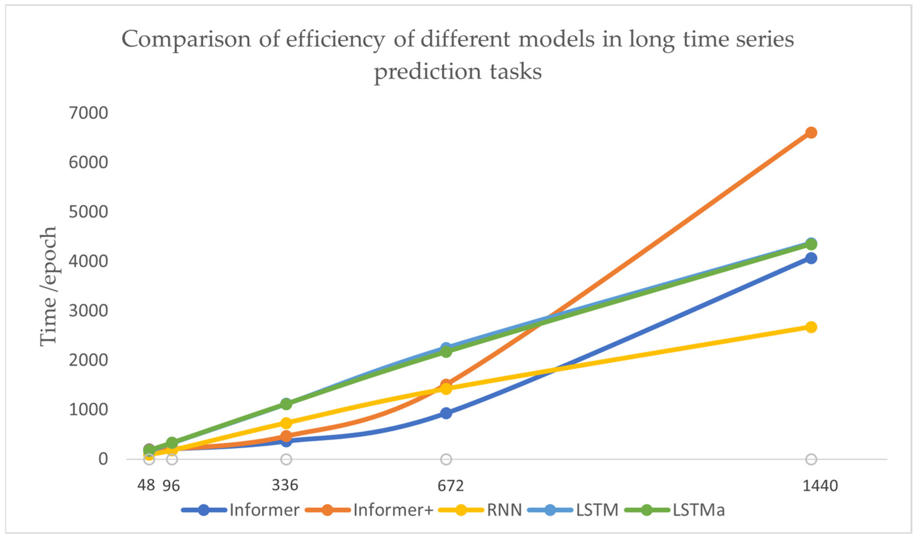
In this paper, we experimentally investigate the optimal solutions of the main parameters in the sparse self-attentive model and compare the optimized parameters with several other common power-load forecasting models using the Nanchang Taoyuan substation dataset. The results of the measured data show that the model based on the sparse self-attentive mechanism has obvious advantages in terms of prediction accuracy and training efficiency compared with the recurrent neural-network-type model, which provides a real case reference under a new solution idea for solving the long-time series power-load forecasting problem.

2. Informer Model

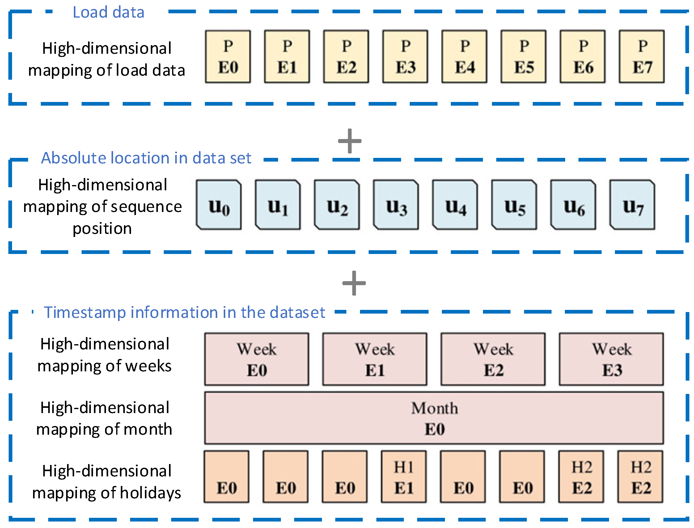
2.1. Input Structure of Informer

In the RNN class of models, the model relies on the cyclic structure as well as timestamps to capture the regularity of the time series. Transformer, on the other hand, relies on the attention mechanism and timestamps to capture the context of the current location. In time-series forecasting problems, global information such as timestamps of different levels (week, month, year) and timestamps of unexpected events (holidays, events) are needed if long-range patterns of data need to be captured. However, this information is difficult to reflect in the self-attention dot product calculation, which tends to cause potential accuracy degradation, so a unified input representation is used in Informer to solve this problem.

In the sparse self-attention model for long-time series power-load forecasting, the input part consists of three components as shown in Figure 1.

Figure 1. Composition structure of Informer model input.

The first step is the mapping of the electric-load data to higher dimensions, which is obtained by one-dimensional convolution of the original data. Next, the position encoding is performed, and the formula for this part is the same as the position encoding in Transformer. The third part is the timestamp information of the data, which is converted into high-dimensional information using a fully connected layer, and finally the above three parts are summed to obtain the final input. As the following equation shows:

$$x_{feed[i]}^t=\alpha u_i^t+P{E}_{(L_x\times (t-1)+i)}+{{\displaystyle {\sum }_p[S{E}_{(L_x\times (t-1)+i)}]}}_p$$

(1)

where $i\in \left\{1,\dots ,L_x\right\}$, α is the hyper parameter used to balance the high-dimensional mapping of the power-load data with the location and timestamp high-dimensional mapping, and α can take the value of 1 if the data have been normalized.

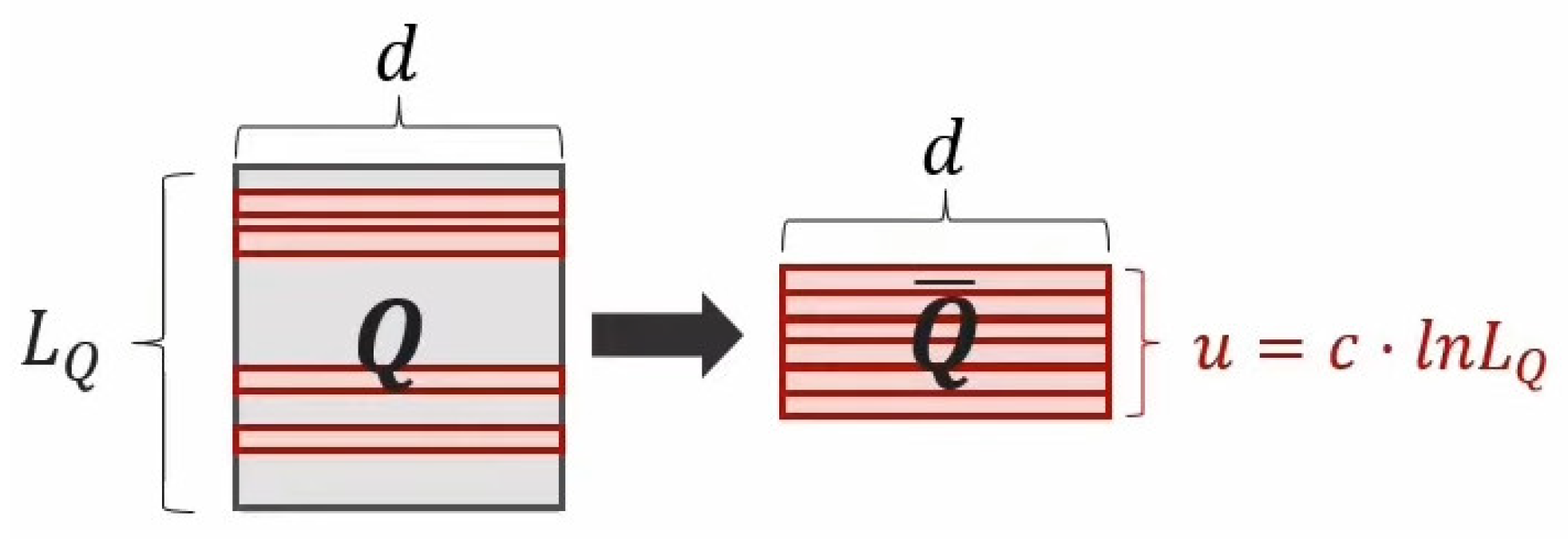
2.2. Self-Attention Mechanism

Self-attention is based on the probability $p(k_j|q_i)$ and combined with Value values to obtain the output, which requires a total of $\mathsf{O}\left(L_Q{L}_K\right)$ memory usage for dot-product computation. To reduce the complexity, a selective counting strategy can be used to count only the attentions that have a large impact on the results. Informer uses the Kullback–Leibler divergence (hereafter KL divergence) to assess the importance of attention.

The formula for KL divergence with the constant term removed can be written as:

$$M\left(q_i,K\right)=\ln {\displaystyle \sum _{j=1}^{L_K}{e}^{\frac{q_i{k}_j{}^T}{\sqrt{d}}}}-\frac{1}{L_K}{\displaystyle \sum _{j=1}^{L_K}\frac{q_i{k}_j^T}{\sqrt{d}}}$$

(2)

The first part of $M\left(q_i,K\right)$ is in Log-Sum-Exp form with respect to q_i, and the second part is the arithmetic mean. If the ith query yields a larger $M\left(q_i,K\right)$, then it is more likely to contain dot-product pairs with dominant positions. Based on the above evaluation, the dot-product pairing computation in the self-attention layer can be sparse by letting only the key and μ dominant queries perform the dot product:

$$\mathrm{Attention}(Q,K,V)=\mathrm{Softmax}\left(\frac{\overline{Q}{K}^T}{\sqrt{d}}\right)V$$

(3)

where $\overline{Q}$ is the matrix after sparsification and has the same size as matrix q. It is combined from the first few with larger weights selected from μ queries after sparsification; μ is controlled by the hyperparameter c, $\mu =c·\ln L_Q$ as shown in Figure 2:

Figure 2. Calculation diagram of $\overline{Q}$.

Such sparse self-attention requires only $\mathsf{O}\left(\ln L_Q\right)$ dot products for query-key lookups, and the memory usage is $\mathsf{O}\left(L_Q\ln L_K\right)$. Because the multi-headed self-attention mechanism is able to capture the features of each dimension, it actually does not cause serious information loss after sparsifying self-attention. However, when iterating over the queries to compute $M\left(q_i,K\right),$ it is necessary to compute the dot product with a complexity of $\mathsf{O}\left(L_Q{L}_K\right)$, which is equivalent to not improving the computational efficiency, so an empirical method is used in Informer to obtain the criteria for query sparsification.

The maximum value of $M\left(q_i,K\right)$ is deduced in Informer:

$$\overline{M}\left(q_i,K\right)=\max \left\{\frac{q_i{k}_j^T}{\sqrt{d}}\right\}-\frac{1}{L_K}{\displaystyle \sum _{j=1}^{L_K}\frac{q_i{k}_j^T}{\sqrt{d}}}$$

(4)

Then the derivation continues through Informer to the following conclusion:

Suppose $k_j$~$\mathcal{N}\left(\mu ,\mathsf{\Sigma }\right)$, let $q{k}_i$ represent $\{(q_i{k}_j^T)/\sqrt{d}|j=1,\dots ,L_K\}$ and $\forall M_{ m}=\mathrm{ma}{x}_{i}M\left(q_i,K\right)$, then there exists $k>0$, $\forall q_1$, $q_2\in \left\{q\right|M\left(q_i,K\right)\in \left[M_m,M_m-k\right)\}$. If $\overline{M}\left(q_1,K\right)>\overline{M}\left(q_2,K\right)$ and $\mathrm{Var}\left(q{k}_1\right)>\mathrm{Var}\left(q{k}_2\right)$, then with high probability $M\left(q_1,K\right)>M\left(q_2,K\right)$.

According to the above conclusion, under the premise that the attention distribution conforms to the long-tail distribution, it is possible not to compute $M\left(q_i,K\right)$ sequentially, but only to randomly sample $U=L_K\ln L_Q$ dot-product pairing for computing $M\left(q_i,K\right)$, and the other dot-product pairings are replaced with 0. This generates the sparse matrix $\overline{\mathrm{Q}}$, and in practice the queries and keys are usually the same, i.e., $L_Q=L_K=L$, then the time complexity and space complexity of the sparse self-attention becomes $\mathsf{O}\left(L\ln L\right)$.

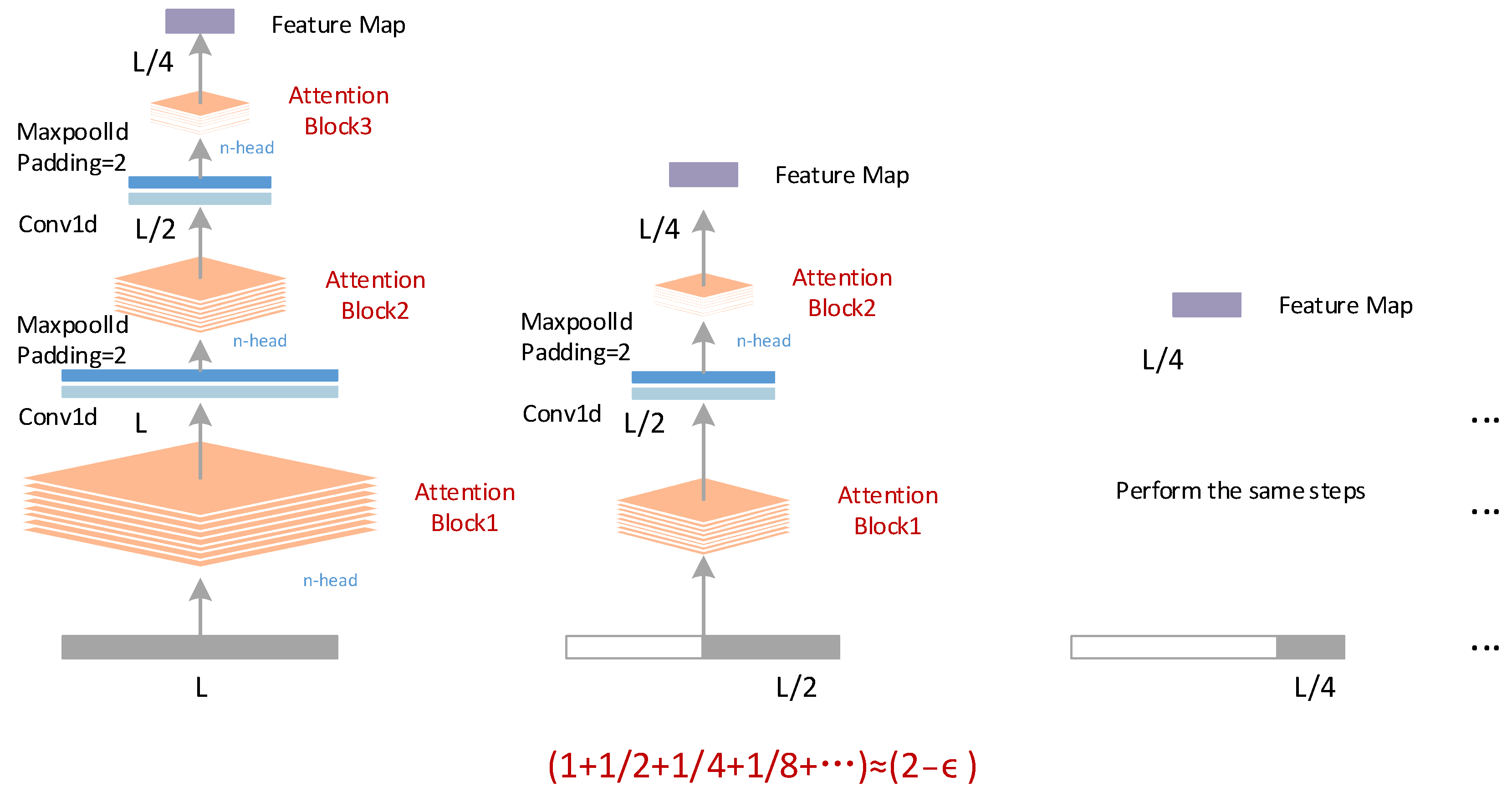
2.3. Distillation Mechanism in the Encoder

As a result of sparse self-attention, the feature map obtained by the encoder contains many redundant combinations of V values, and the feature map can be reduced by extracting some dominant features through convolution and pooling, a step called Distilling in Informer [27]. The equation for the distillation operation to transform layer j to layer j + 1 is as follows:

$${\mathrm{X}}_{j+1}^{\mathrm{t}}=\mathrm{MaxPool}\left(\mathrm{ELU}\left(\mathrm{Conv}1d\left({\left[{\mathrm{X}}_{\mathrm{j}}^{\mathrm{t}}\right]}_{\mathrm{AB}}\right)\right)\right)$$

(5)

where ${\left[.\right]}_{\mathrm{AB}}$ represents the attention block, which is exactly the same structure as the attention block in Transformer, except that the multi-headed self-attention layer is replaced by a sparse multi-headed self-attention layer. Figure 3 shows the structure of the encoder part.

Figure 3. Encoder for Informer.

The light blue layer represents the Conv1d convolutional layer, which uses the ELU activation function to perform one-dimensional convolution in the time dimension and then pooling so that it downsamples to 1/2 of the original length. To improve the robustness of the distillation operation and to prevent excessive information loss, the input is copied at the beginning and only half of it is taken at a time, and then the output of the feature map is aligned by gradually reducing one attention block. The length of the sequence for each copy is L, 1/2 L, 1/4 L, 1/8 L… summed to 2 − ϵ, i.e., the memory usage is $\mathsf{O}\left(\left(2-ϵ\right)\mathrm{LlnL}\right)$. The output feature maps are stitched and aligned to obtain the final output hidden layer of the encoder.

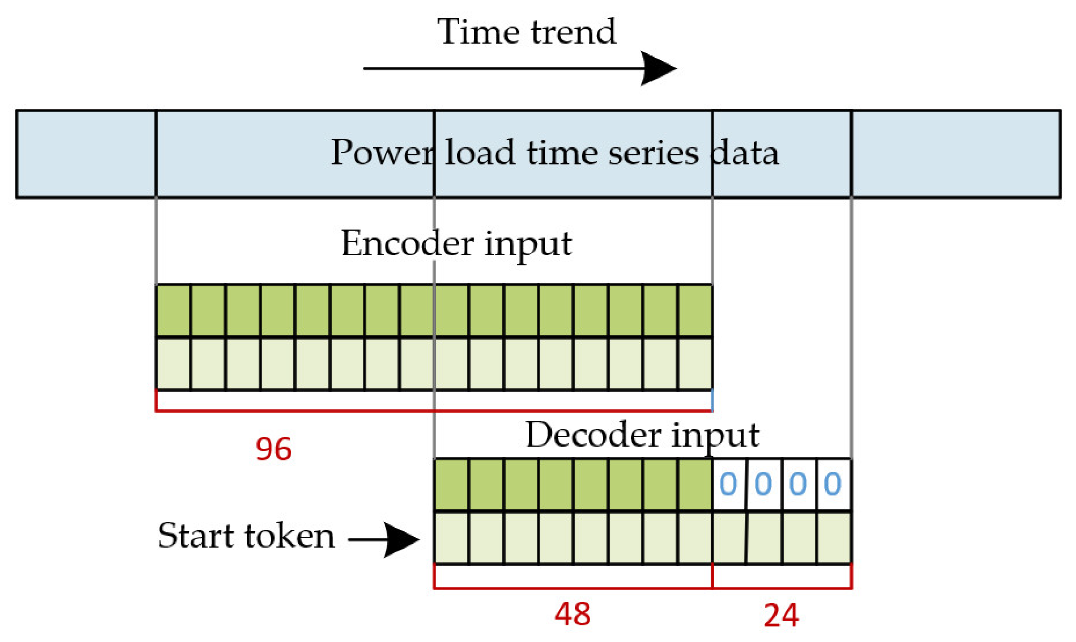
2.4. One-Step Generative Decoder

In Informer, the decoder is similar to the decoder in Transformer and contains two identical multi-headed self-attention layers. Inspired by the effective use of Start-token in natural language dynamic decoders [28], Informer also uses Start-token here to turn dynamic output results into one-step generation results. Masked multi-headed attention is applied in sparse self-attentiveness by setting a mask on the dot product. The mask in the decoder is a lower triangular matrix, and the mask enables the model to obtain only the already predicted results and not the later unpredicted results, which can prevent the model from self-regression.

Enter the following parameters into the decoder:

$$X_{\mathrm{de}}^t=\mathrm{Concat}\left(X_{\mathrm{token}}^t,X_0^t\right)\in {ℝ}^{\left(L_{\mathrm{token}}+L_y\right)\times d_{\mathrm{model}}}$$

(6)

where $X_{\mathrm{to}ken}^t\in {ℝ}^{L_{token}\times d_{model}}$ stands for Start-token, which can also be interpreted as the sequence to be predicted, and $X_0^t\in {ℝ}^{L_y\times d_{model}}$ is the target sequence here all set to 0 as a placeholder. Instead of using a particular flag as a token, here L__token of them are copied from the input sequence as the Start-token, for example, the previous segment of the output sequence.

Figure 4 shows the schematic diagram of Start-token.

Figure 4. Calculation diagram of $\overline{Q}$ schematic diagram of Start-token in decoder.

At this point, the overall structure of Informer has been introduced, and the structure of the model is shown in Figure 5:

Figure 5. Overall structure of Informer.

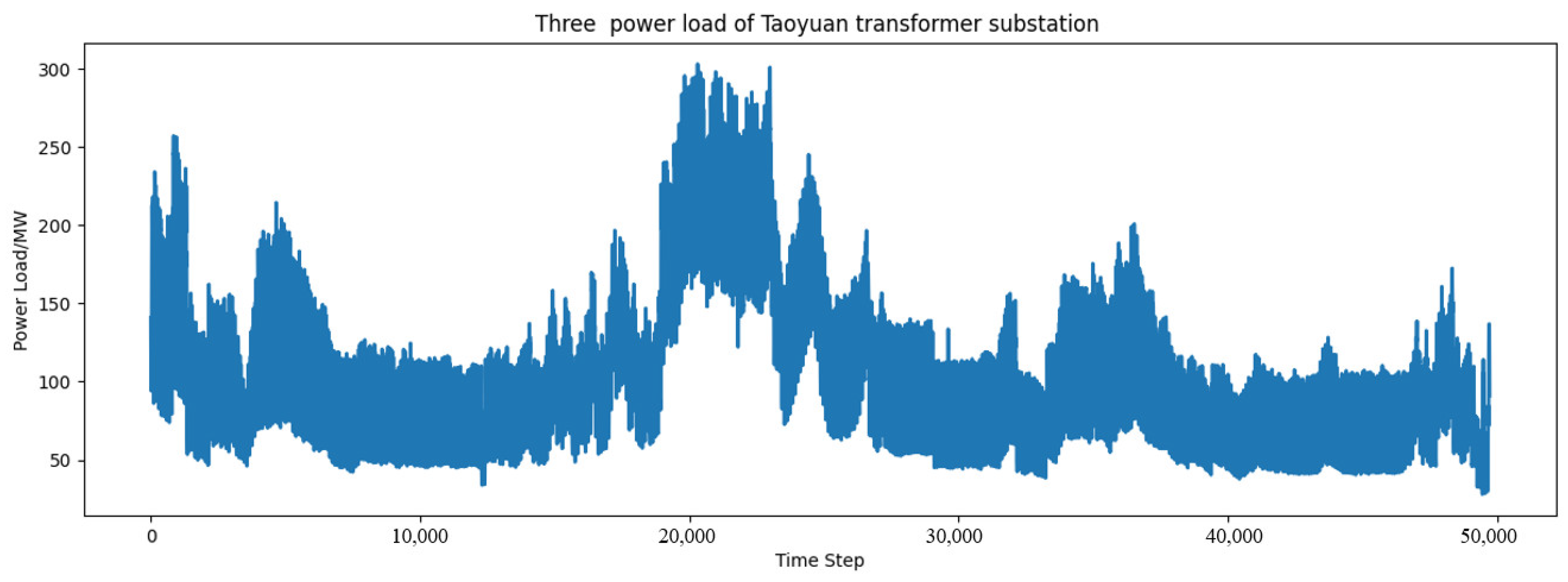
3. Data Correlation Analysis

This paper selects the power-load data of Taoyuan substation in Nanchang City. The dataset spans 1 January 2019 to 1 June 2020, sampling every 15 min and sampling 96 points a day for a total of 49,720 electrical load data. This dataset is a highly refined dataset compared to common power-load datasets and is suitable for exploring the performance of the model in long-time series power-load forecasting. The dataset comes from the online grid platform of the National Grid, which can guarantee the authenticity and reliability of the data. Since this paper is to investigate the performance of the proposed improved models for long-term load forecasting, only a single factor of electric load is considered for all models, and no other environmental factors are considered.

Taoyuan substation is a 220 kV substation with two main transformers of 180 MVA capacity, carrying the power supply load of 110 kV substations such as Tengwangge, Chaoyang, Fengshan, Xihu, Taoyuan and Yunfei. The load area of Taoyuan is the old city of Nanchang, which is a typical urban civil load and commercial load.

The power-load data of Taoyuan substation were pre-processed and the full picture of the dataset was drawn after correcting the abnormal data as shown in Figure 6. It can be seen that the load data of Taoyuan substation have obvious seasonal periodicity, showing high load in summer and winter, low load in autumn and spring and peak of electric load in summer.

Figure 6. Data overview of Nanchang Taoyuan substation.

The autocorrelation coefficient is the degree of correlation between the same event in different periods. It can also be understood as the correlation between the past and present of the same individual. The equation for the autocorrelation coefficient is shown in Equation (7):

$$\rho \left(\mathrm{t},s\right)=\frac{E(x_t-{\mu }_t)(x_s-{\mu }_s)}{\sqrt{D{x}_t{x}_s}}$$

(7)

where E is the expectation, D is the variance.

Electricity load is somewhat cyclical, following the previous rule of variation, and the load data within a certain period have a certain correlation. Due to the large dataset, in order to explore the autocorrelation of electric loads, Figure 7 selects the load data of Taoyuan substation in Nanchang City, which records the electric-load data every 15 min, and selects 1440 data, i.e., one month’s electric load, and draws the following electric-load autocorrelation coefficient graph.

Figure 7. Autocorrelation coefficient diagram of power load of Taoyuan substation in Nanchang.

The closer the correlation coefficient is to 1, the greater is the correlation. From the figure, it can be seen that the electric load shows a high correlation between adjacent points; in particular, the autocorrelation coefficient is as high as 0.9 between all five adjacent points, as shown in Table 1.

Table 1. Correlation analysis of power load in five adjacent time steps.

Delay	Autocorrelation	True Value	Ljung-Box Test
1	0.995	140.83	1429.059
2	0.984	133.18	2826.708
3	0.966	127.61	4176.199
4	0.943	023.99	5462.566
5	0.915	119.26	6673.302

The light blue area of Figure 6 shows the 95% confidence interval, and the autocorrelation coefficient still exceeds the 95% confidence interval after 294 lag steps, with a strong correlation. Over time, the autocorrelation coefficient shows a cyclical ebb and flow, trailing a downward trend and eventually, slowly converging to 0 at around 1440 points. This also indicates that the power load is correlated over a long period of time. If the law of long-time series power load can be accurately captured, better long-time series power-load prediction can be achieved [29], which provides the theoretical basis for long-time series with Nanchang Taoyuan substation dataset.

4. Example Analysis

4.1. Model Parameter Optimization

The experiments in this section were conducted on an Inter Xeon(R) Silver 4214R CPU, 256 GB of RAM, and two RTX6000s for a total of 40 GB of RAM on hardware platform.

In order to ensure that the model does not overload the memory even at the maximum prediction length, and because this experiment is a comparison experiment and does not pursue absolute accuracy, the selected value of Batch Size is 8 for all models, and the models in this paper all use EarlyStopping to dynamically select Epochs. The Patience value is set to 3, i.e., the val_loss value is greater than val_loss for three consecutive times. At loss minimum, the training is terminated and the minimum value is taken.

The structure of the improved sparse self-attentive model is shown in Table 2, and the experiments in this subsection are all based on the model with the following parameters.

Table 2. Improved structure of sparse self-attentive model.

Encoder			N
Input	1 × 3 Conv1d	Embedding (d = 512)	6
Sparse self-attention blocks	Multi-head Sparse Attention (h = 16, d = 32)
	Add, LayerNorm, Dropout (p$=0.1$)
	Pos-wise FFN ($d_{inner}=2048$), GELU
	Add, LayerNorm, Dropout (p $=0.1$)
Distillation layer	1 × 3 Conv1d
	Max pooling (stride = 2)
Decoder			N
Input	1 × 3 Conv1d	Embedding (d = 512)	6
Masked SAB	Add a mask to the Attention Block
Self-attention block	Multi-head Sparse Attention (h = 8, d = 64)
	Add, LayerNorm, Dropout (p $=0.1$)
	Pos-wise FFN ($d_{inner}=2048$), GELU
	Add, LayerNorm, Dropout (p $=0.1$)
Distillation layer	1 × 3 Conv1d
	Max pooling (stride = 2)
Output	FCN ($\mathrm{d}=d=d_{out}$)

To facilitate comparison of experimental results, all data were first normalized to the 0–1 interval using the MinMaxScaler method for all data. Considering the balance of memory and accuracy, Batch Size was selected as 8.

(1)

The effect of the length of the input data on the prediction results

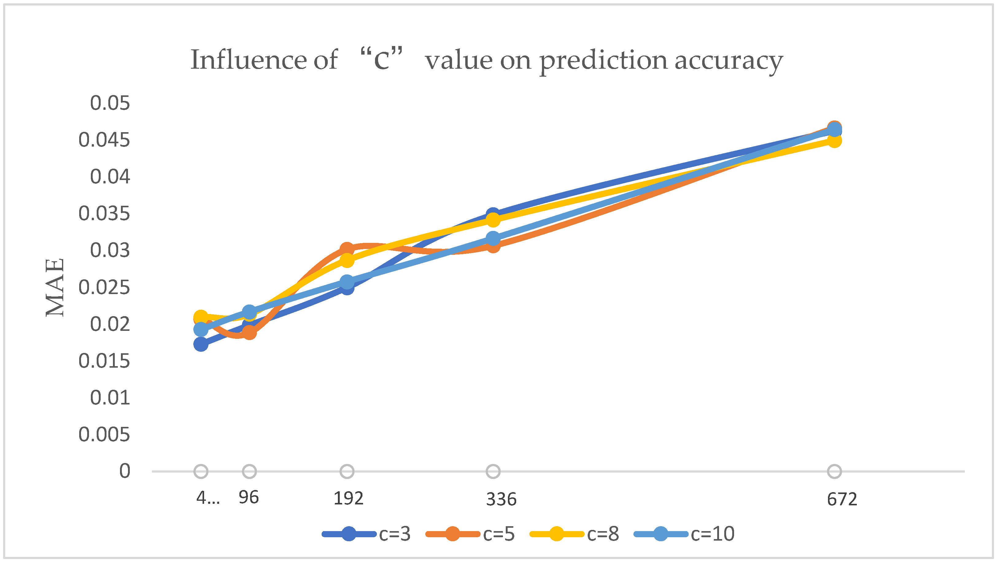
With more samples input at once during training, the model is theoretically better able to capture the long-range patterns between data. However, too much input inevitably makes the model’s overhead on memory increase significantly and the training time increases significantly, so a balance needs to be found between these. The experimental results are shown in Table 3:

Table 3. Effects of different input–output ratios on model performance.

Predicted Length	288			672
Input Length	288	576	1152	672	1344	2688
RMSE	0.044	0.046	0.060	0.079	0.073	0.070
MAE	0.032	0.033	0.037	0.047	0.046	0.049
Time	312	770	2613	930	3510	13,384

From the experimental results, it can be seen that more input data do not have the effect of improving the training accuracy while reducing the efficiency of the model. Here it is speculated that the model may be due to the fact that too much data in refining the data law not only do not provide a more long-range law but also add a great deal of interference terms, leading to a decrease in training accuracy. Therefore, the number of input time points and the number for prediction time are taken as the same value in the subsequent training, which can guarantee the prediction accuracy and improve the efficiency to the best.

(2)

The effect of hyperparameter c on the experiment

The number of times to calculate the dot-product pairing is determined by μ, which is determined by the hyperparameter c, i.e., $\mu =c·\ln L_Q$. An increase in the value of c means that the number of dot-product calculations is also increasing, which then inevitably leads to an increase in prediction accuracy and a decrease in prediction efficiency. In order to investigate the effect of the hyperparameter c on the results in the following experiments were carried out on c. The experimental results are shown in Table 4.

Table 4. Influence of different C values on model performance.

C	Metric	48	96	192	336	672
3	RMSE	0.0262	0.0320	0.0366	0.0479	0.0691
	MAE	0.0173	0.0199	0.0250	0.0349	0.0463
	Time	196	205	243	342	916
5	RMSE	0.0289	0.0307	0.04060	0.0441	0.0786
	MAE	0.0207	0.0189	0.0302	0.0307	0.0467
	Time	197	209	246	365	938
8	RMSE	0.0306	0.0333	0.0402	0.0495	0.0725
	MAE	0.0210	0.0214	0.0287	0.0342	0.0450
	Time	199	212	249	376	961
10	RMSE	0.0275	0.0344	0.0379	0.0458	0.0814
	MAE	0.0193	0.0217	0.0258	0.0317	0.0465
	Time	200	210	246	376	849

The above data are plotted as a scatter plot as shown in Figure 8:

Figure 8. Prediction accuracy of Informer under different C values.

From the perspective of computational efficiency, the number of dot-product operations increases as the value of c increases, but the selection of c value has limited effect on the computational efficiency from the experimental results. Considering the computational efficiency and computational accuracy, c is taken as 5 in all subsequent experiments.

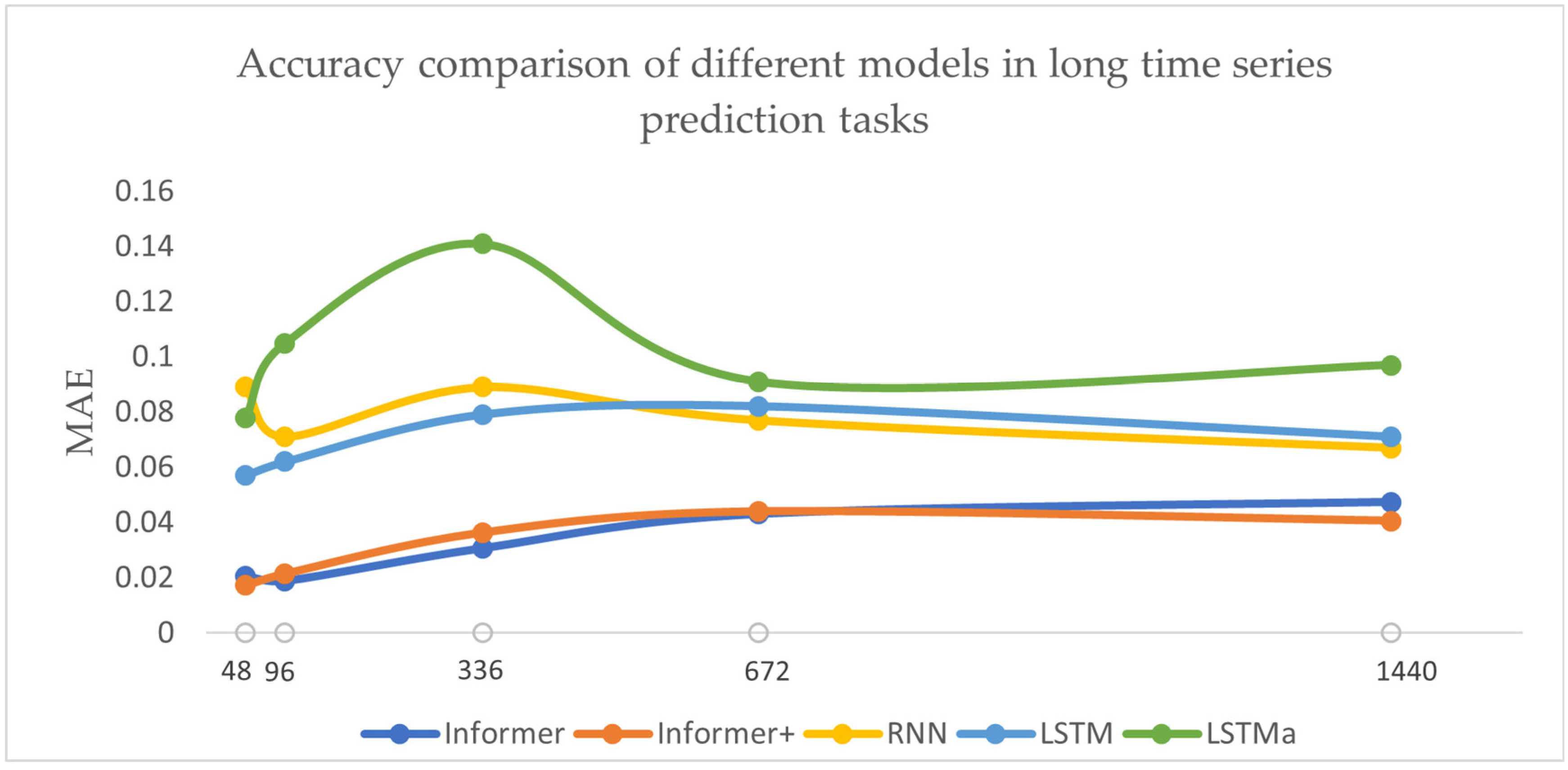
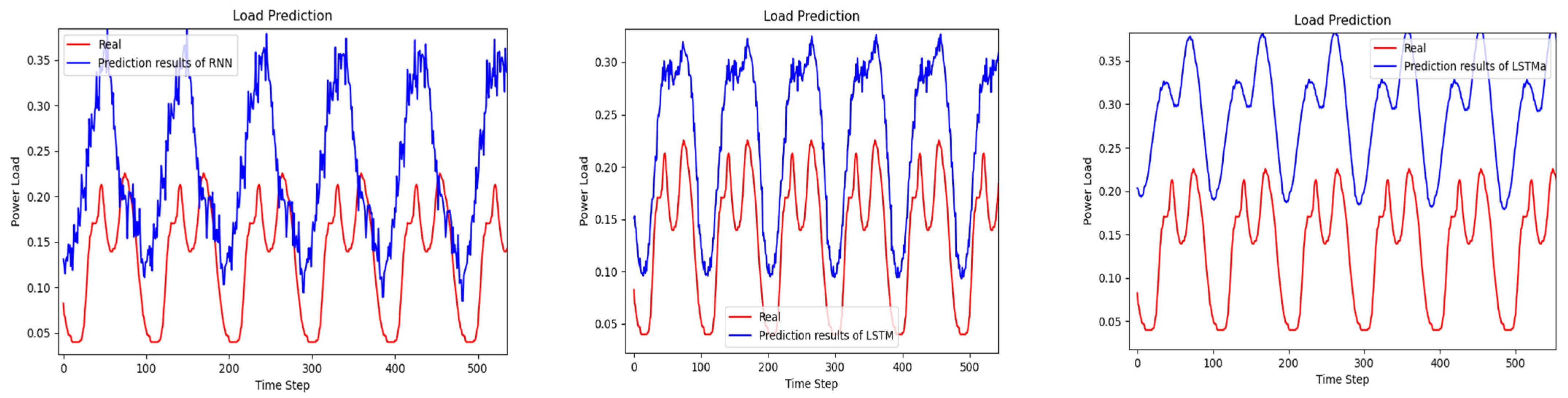
4.2. Experimental Results

This section next introduces other models as a baseline to explore whether there is some advantage of Informer and Informer+ with the distillation mechanism removed for the power-load forecasting task with optimal parameters. In this section, LSTM, RNN and LSTM with the attention mechanism added (LSTMa) were selected for comparison. The experimental results are as shown in Table 5:

Table 5. Performance of different models in power-load forecasting.

Methods	Metric	48	96	336	672	1440
Informer	RMSE	0.0289	0.0307	0.0441	0.0714	0.0670
	MAE	0.0207	0.0189	0.0307	0.0431	0.0474
	Time	197	209	365	930	4070
Informer+	RMSE	0.0255	0.0303	0.0508	0.0748	0.0583
	MAE	0.0173	0.0216	0.0364	0.0440	0.0406
	Time	186	204	463	1508	6610
RNN	RMSE	0.108	0.090	0.108	0.093	0.084
	MAE	0.089	0.071	0.089	0.077	0.067
	Time	92	176	730	1421	2674
LSTM	RMSE	0.069	0.072	0.089	0.093	0.081
	MAE	0.057	0.062	0.079	0.082	0.071
	Time	166	330	1117	2249	4365
LSTMa	RMSE	0.095	0.124	0.169	0.103	0.122
	MAE	0.078	0.105	0.141	0.091	0.097
	Time	181	331	1116	2169	4346

The above data are plotted as a scatter plot as shown in Figure 9:

Figure 9. Accuracy comparison of five models in power-load forecasting.

From the experimental results, we can see that the training accuracy of Informer and Informer+ is significantly improved compared to the RNN, LSTM and LSTMa models. Informer and Informer+ showed excellent prediction performance on the 0–672 step prediction task and significantly outperformed other models in terms of prediction accuracy on longer time-series-prediction tasks. The prediction accuracy of both models decreased with increasing time steps until the prediction slowly stabilized after 672 time steps. However, due to the limited conditions, it was not possible to conduct a longer time-step test, so the prediction performance after 1440 points is not discussed in this paper.

Figure 10 and Figure 11 show the predicted results of the five models above compared to the true values at 500 time steps of prediction. The comparison graphs show visually that the two models Informer and Informer+, which are based entirely on the self-attention mechanism, fit the load curves more accurately, and the predicted and true values show a consistent trend, while the predicted values of RNN, LSTM and LSTMa based on recurrent neural networks were significantly higher than the true values. The LSTMa model had a higher MAE score than RNN and LSTM but was smoother than the above two models, fluctuated synchronously with the real load, and was significantly more usable than the RNN and LSTM models after data correction in the vertical direction.

Figure 10. Prediction results of the model based on RNN in 500 time steps.

Figure 11. Prediction results of Informer-based model in 500 time steps.

In terms of computational efficiency, RNN, LSTM and LSTMa can all be expressed in an approximately linear relationship between the number of prediction steps and the prediction time due to their serial computation characteristics and the nature of the distance between points as L. The RNN model benefits from its simplest structure and has a significantly lower slope of prediction-time rise with increasing prediction time steps than the LSTM as well as the LSTMa. The prediction time-step–time relationship curves for Informer and Informer+ are a concave function, and it can be approximated from the measured data that the efficiency of Informer is higher than the other models mentioned above within a certain prediction time step. This interval is defined here as the high-efficiency interval, which is of great practical significance in practical engineering. It can be seen from Figure 12 that the high-efficiency interval for both Informer and Informer+ is higher than 672 time steps. If 96 data are available in a day, it corresponds to more than one week of power-load data, which is sufficient to cover most short-term power-load forecasting scenarios. The predicted time-step–time relationship curve of Informer+ also presents a concave function, but the slope of the training-time rise with increasing time steps is much larger than that of Informer because of the reduced distillation operation, which results in a larger amount of data. This makes Informer+ significantly less efficient as the predicted time points increase, and less effective than Informer in practical engineering applications.

Figure 12. Efficiency comparison of five models in power-load forecasting.

Combining the above analysis of prediction accuracy and prediction efficiency, in this paper the proposed Informer-based model effectively achieves higher accuracy in long-time series power-load forecasting. In terms of long-time series power-load prediction, the accuracy of the proposed Informer-based model is significantly improved compared to the RNN, LSTM and LSTMa models by experimenting with the Taoyuan substation dataset. In addition, the proposed Informer-based model has certain advantages over RNN, LSTM and LSTMa in terms of training efficiency within a certain prediction time step. The research content of this paper has certain academic significance and engineering value.

5. Conclusions

In this paper, the Informer model was used for electricity-load forecasting and was compared with three models based on recurrent neural networks. Experiments showed that Informer’s prediction accuracy within 1440 time steps on the power-load dataset of Nanchang Taoyuan substation was significantly higher than that of the three models based on recurrent neural networks, which can provide more refined predictions to cope with more complex application scenarios requiring higher load prediction. At the same time, Informer has a significantly higher prediction efficiency than recurrent neural network models in a certain time step due to its parallel advantage. Informer has a large potential in the field of power-load forecasting. In addition, Informer also demonstrates satisfactory performance in long-time series power-load forecasting, which can provide some guidance for long-term planning of the grid system.

The performance of the proposed model will be further explored in a better experimental environment, as the “Batch Size” was too large due to the limitation of the experimental hardware equipment, resulting in insufficient memory. In addition, this dataset contained only the electrical-load data, and the performance of the model will be further investigated by incorporating other environmental and other influencing factors. In the future, we will also try to apply the proposed model to other fields such as photovoltaic and wind power, and make some optimization improvements to the model based on the latest research.

References

- Zhu, J.C.; Yang, Z.L.; Guo, Y.J.; Yu, K.J.; Zhang, J.K.; Mu, X.M. A review on the application of deep learning in power load forecasting. J. Zhengzhou Univ. 2019, 40, 13–22. [Google Scholar]
- Li, Y.; Jia, Y.J.; Li, L.; Hao, J.; Zhang, X. Short-term electric load forecasting based on random forest algorithm. Power Syst. Prot. Control. 2020, 48, 117–124. [Google Scholar]
- Zhuang, S.J.; Yu, Z.Y.; Guo, W.Z.; Huang, F.W. Cross-scale recurrent neural network based on Zoneout and its application in short-term power load forecasting. Comput. Sci. 2020, 47, 105–109. [Google Scholar]
- Jingliang, Y.; Linhai, Q.; Shun, T.; Hong, W. Attention LSTM-based optimization of on-load tap-changer operation. Power Grid Technol. 2020, 44, 2449–2456. [Google Scholar]
- Lv, H.C.; Wang, W.F.; Zhao, B.; Zhang, Y.; Guo, Q.T.; Hu, W. Short-term station load forecasting based on Wide&Deep LSTM model. Power Grid Technol. 2020, 44, 428–436. [Google Scholar]
- Kong, W.; Dong, Z.Y.; Jia, Y.; Hill, D.J.; Xu, Y.; Zhang, Y. Short-term residential load forecasting based on LSTM recurrent neural network. IEEE Trans. Smart Grid 2017, 10, 841–851. [Google Scholar] [CrossRef]
- Lee, C.M.; Ko, C.N. Short-term load forecasting using lifting scheme and ARIMA models. Expert Syst. Appl. 2011, 38, 5902–5911. [Google Scholar] [CrossRef]
- Fan, C.; Ding, Y. Cooling load prediction and optimal operation of HVAC systems using a multiple nonlinear regression model. Energy Build. 2019, 197, 7–17. [Google Scholar] [CrossRef]
- Zheng, T.; Girgis, A.A.; Makram, E.B. A hybrid wavelet-Kalman filter method for load forecasting. Electr. Power Syst. Res. 2000, 54, 11–17. [Google Scholar] [CrossRef]
- Krizhevsky, A.; Sutskever, I.; Hinton, G.E. Imagenet classification with deep convolutional neural networks. Commun. ACM 2017, 60, 84–90. [Google Scholar] [CrossRef]
- Jingbo, M.; Honggeng, Y. Application of adaptive Kalman filtering in short-term load forecasting of power systems. Power Grid Technol. 2005, 29, 75–79. [Google Scholar]
- Quan, L. Adaptive Kalman filter-based load forecasting under meteorological influence. Comput. Meas. Control. 2020, 28, 156–159 + 165. [Google Scholar]
- Xu, W.; Peng, H.; Zeng, X.; Zhou, F.; Tian, X.; Peng, X. A hybrid modelling method for time series forecasting based on a linear regression model and deep learning. Appl. Intell. 2019, 49, 3002–3015. [Google Scholar] [CrossRef]
- Liu, L.; Liu, J.; Zhou, Q.; Qu, M. An SVR-based Machine Learning Model Depicting the Propagation of Gas Explosion Disaster Hazards. Arab. J. Sci. Eng. 2021, 46, 10205–10216. [Google Scholar] [CrossRef]
- Ning, Y.; Yong, L.; Yong, W. Short-term power load forecasting based on SVM. In Proceedings of the World Automation Congress 2012, Puerto Vallarta, Mexico, 24–28 June 2012. [Google Scholar]
- Che, J.; Wang, J. Short-term load forecasting using a kernel-based support vector regression combination model. Appl. Energy 2014, 132, 602–609. [Google Scholar] [CrossRef]
- Hsu, Y.Y.; Ho, K.L. Fuzzy linear programming: An application to short-term load forecasting. Gener. Transm. Distrib. IEEE Proc. C 1992, 139, 471–477. [Google Scholar] [CrossRef]
- Zhaoyu, P.; Shengzhu, L.; Hong, Z.; Nan, Z. The application of the PSO based BP network in short-term load forecasting. Phys. Procedia 2012, 24, 626–632. [Google Scholar] [CrossRef]
- Bashir, Z.A.; El-Hawary, M.E. Applying waveletsto short-term load forecasting using PSO-based neural networks. IEEE Trans. Power Syst. 2009, 24, 20–27. [Google Scholar] [CrossRef]
- Vaswani, A.; Shazeer, N.; Parmar, N.; Uszkoreit, J.; Jones, L.; Gomez, A.N.; Kaiser, Ł.; Polosukhin, I. Attention is all you need. Adv. Neural Inf. Process. Syst. 2017, 30. [Google Scholar]
- Yao, L.; Jie, Y.; Zhijuan, S.; Congcong, Z. Robust PM2.5 prediction based on stage-based time-series attention network. Environ. Eng. 2021, 39, 93–100. [Google Scholar] [CrossRef]
- Kitaev, N.; Kaiser, Ł.; Levskaya, A. Reformer: The Efficient Transformer [EB/OL]. Available online: https://arxiv.org/pdf/2001.04451.pdf (accessed on 11 March 2020).
- Child, R.; Gray, S.; Radford, A.; Sutskever, I. Generating Long Sequences with Sparse Transformers. arXiv 2019, arXiv:1904.10509. [Google Scholar]
- Beltagy, I.; Peters, M.E.; Cohan, A. Longformer: The Long-Document Transformer. arXiv 2020, arXiv:2004.05150. [Google Scholar]
- Li, S.; Jin, X.; Xuan, Y.; Zhou, X.; Chen, W.; Wang, Y.; Yan, X. Enhancing the Locality and Breaking the Memory Bottleneck of Transformer on Time Series Forecasting. Adv. Neural Inf. Process. Syst. 2019, 32, abs/1907.00235. [Google Scholar]
- Zhang, H.; Jiang, Y. Axle temperature prediction model for urban rail vehicles based on sparse attention mechanism. Technol. Innov. 2021, 3, 1–4. [Google Scholar] [CrossRef]
- Zhou, H.; Zhang, S.; Peng, J.; Zhang, S.; Li, J.; Xiong, H.; Zhang, W. Informer: Beyond Efficient Transformer for Long Sequence Time-Series Forecasting. Proc. AAAI Conf. Artif. Intell. 2020, 35, 11106–11115. [Google Scholar] [CrossRef]
- Yu, F.; Koltun, V.; Funkhouser, T. Dilated residual networks. In Proceedings of the IEEE Conference on Computer Vision and Pattern Recognition (CVPR), Honolulu, HI, USA, 21–26 July 2017; pp. 472–480. [Google Scholar]
- Lindberg, K.B.; Seljom, P.; Madsen, H.; Fischer, D.; Korpås, M. Long-term electricity load forecasting: Current and future trends. Util. Policy 2019, 58, 102–119. [Google Scholar] [CrossRef]
Disclaimer/Publisher’s Note: The statements, opinions and data contained in all publications are solely those of the individual author(s) and contributor(s) and not of MDPI and/or the editor(s). MDPI and/or the editor(s) disclaim responsibility for any injury to people or property resulting from any ideas, methods, instructions or products referred to in the content. |
© 2023 by the authors. Licensee MDPI, Basel, Switzerland. This article is an open access article distributed under the terms and conditions of the Creative Commons Attribution (CC BY) license (https://creativecommons.org/licenses/by/4.0/).