Article

Ground Fault Detection Based on Fault Data Stitching and Image Generation of Resonant Grounding Distribution Systems

1
College of Electrical Engineering, Guizhou University, Guiyang 550025, China
2
Electric Power Research Institute of Guizhou Power Grid Co., Ltd., Guiyang 550002, China
*
Authors to whom correspondence should be addressed.
Energies 2023, 16(7), 2937; https://doi.org/10.3390/en16072937
Submission received: 21 February 2023 / Revised: 13 March 2023 / Accepted: 21 March 2023 / Published: 23 March 2023
(This article belongs to the Special Issue Modern Power System Stability and Optimal Operating)

Abstract

:
Fast and accurate fault detection is important for the long term, stable operation of the distribution network. For the resonant grounding system, the fault signal features extraction difficulties, and the existing detection method’s accuracy is not high. A ground fault detection method based on fault data stitching and image generation of resonant grounding distribution systems is proposed. Firstly, considering the correlation between the transient zero-sequence current (TZSC) of faulty and healthy feeders under the same operating conditions, a fault data stitching method is proposed, which splices the transient zero-sequence current signals of each feeder into system fault data, and then converts the system fault data into grayscale images by combining the signal-to-image conversion method. Then, an improved convolutional neural network (CNN) is used to train the grayscale images and then implement fault detection. The simulation results show that the proposed method has high accuracy and strong robustness compared with existing fault detection methods.

1. Introduction

When a single-phase ground (SPG) fault occurs in a resonant grounding system, it is allowed to continue operation for about 1 to 2 h, according to the regulations. However, with the passage of operation time [1], phase short circuits and power supply interruption may occur, which seriously affect the power supply reliability of the power system. Therefore, fast and reliable fault detection has become a basic requirement for modern distribution networks [2]. For the complex fault situation of the resonant grounding system, where the fault current is susceptible to arcing, noise and other factors, fast and accurate fault detection is of great significance for the long-term reliable and stable operation of the distribution network.
Existing SPG fault detection methods for resonant grounding systems are mainly classified into steady-state methods [3,4,5,6], transient methods [7,8,9], and data-driven methods [10,11,12,13,14,15,16]. The steady-state method often uses fault characteristics such as phase, amplitude, and the fifth harmonic of the zero-sequence current to achieve fault detection. However, the steady-state method is not obvious in the case of fault conditions or changes in the network structure fault characteristics, which can easily lead to errors in feeder detection. The transient method has received a lot of attention from scholars because of its rich information on fault characteristics, compared with the steady-state method. Transient methods often use digital signal processing methods such as variational mode decomposition (VMD), Hilbert–Huang transform (HHT), wavelet transform (WT), and S-transform to extract single or multiple fault features of TZSC to improve fault detection accuracy. However, fault features extracted based on digital signal processing methods rely heavily on fusion theory and human experience, and lack completeness [10]. With the development of the digital power grid, the digitalization and intelligence level of the distribution system will be improved, and the data-driven method based on the data is expected to make up for the shorfalls in the transient method.
Machine learning (ML) methods use digital signal processing methods to extract multidimensional fault features of transient zero-sequence currents to compensate for the shortcomings of single fault features to improve the characterization ability of fault features. Ghaderi et al. [11] extracted the current waveform energy and normalized the joint time-frequency matrix input to a support vector machine to implement fault detection. M. Sahani et al. [12] used VMD to extract the corresponding amplitude standard deviation, energy, Rényi entropy, and crest factor from the current as feature vectors for fault detection. Deep learning (DL) methods use digital signal methods to convert time-domain signals into time-frequency domain signals to obtain more useful fault information as a way to enhance the characterization of fault features. Guo et al. [13] used HHT bandpass recording filters for faulty signals to construct the time-frequency energy matrix and used the time-frequency energy matrix as an input to the CNN. Wang et al. [14] obtained a wavelet coefficient energy matrix image of the fault signal by WT to obtain the fault information in the frequency domain. In terms of classification method improvement, the detection accuracy of deep learning models such as CNN and LSTM was better than that of shallow learning methods such as SVM and extreme learning machine (ELM) [15,16]. However, the fault features processed or extracted by signal processing methods may exhibit strong uncertainties and randomness, which are hardly applicable to all fault conditions, especially extreme fault conditions, such as high impedance and strong noise [17]. In other words, which feature extraction method is the best choice for faulty signals still has no concrete answer [18]. Therefore, the limitations of the signal processing method can affect the robustness of the detection model.
In summary, the existing data-driven detection methods still have the following problems: (1) the existing methods have insufficient feature characterization capability; (2) the limitations of the digital signal processing methods can lead to poor robustness of the models. To address the above issues, in this study, a fault data stitching and image generation method is proposed, which stitches TZSC of each feeder into a system fault signal and then converts it into a grayscale image. This method has the advantage of small computational effort compared to existing fault detection methods and eliminates the influence of expert experience as much as possible. Then, the proposed improved CNN can adaptively extract the features of these grayscale images. The simulation results show that the proposed method has high accuracy and robustness in fault detection.
The main contributions of this paper are summarized in the following three points. First, a fault data stitching and image generation method is proposed, which enhances the characterization of fault features. Second, an improved CNN model is proposed to speed up the training of convolutional neural networks and reduce the sensitivity to network initialization using the BN method [19]. Third, the proposed method is compared with existing feeder detection methods in this paper to demonstrate the effectiveness of the proposed method.
The subsequent structure of this paper is as follows: Section 2 provides a detailed analysis of the existing data-driven fault detection-based methods and their limitations. The fault data stitching and image generation methods are elaborated in Section 3. Section 4 provides experiments and a discussion to verify the effectiveness of the proposed method through comparative experiments. Section 5 summarizes the proposed method in this paper.

2. Related Studies

Currently, existing data-driven fault detection methods based on data can be broadly classified into two types, which are referred to as Option 1 and Option 2 in this paper. This section analyzes these two options and discusses their limitations.

2.1. Option 1

Option 1 is a manual feature extraction, combined with the classifier method. This method used a mathematical signal processing method to extract time-domain, frequency-domain and energy-domain features corresponding to zero-sequence current, and inputs the ML algorithm to realize fault detection, as shown in Figure 1. Due to the complex fault conditions and susceptibility to noise, a single fault feature has difficulty meeting the requirements of fault detection accuracy, and Option 1 extracts multiple features by digital signal processing methods to improve fault detection accuracy.
In [20], an adaptive neuro-fuzzy inference systems (ANFISs)-based fault classification method for distribution systems was proposed. Seven fault identifiers were extracted from the fault components of transient zero-sequence voltage and three-phase current by using FFT and discrete wavelet transform. We input these fault identifiers into the trained ANFISs to obtain the fault type. Adewole et al. [21] used discrete wavelet transform (DWT) to decompose the fault transient signals and calculate per-unit entropy as fault features, which were input to ANN for fault detection and localization. Although good detection results can be obtained in Option 1, it has two drawbacks: (1) the extracted two or more features only reflect certain aspects of the transient current, which is prone to missing fault features; (2) most word signal processing methods use fixed-basis functions, which have a limited ability to enhance the feature characterization of the original data.

2.2. Option 2

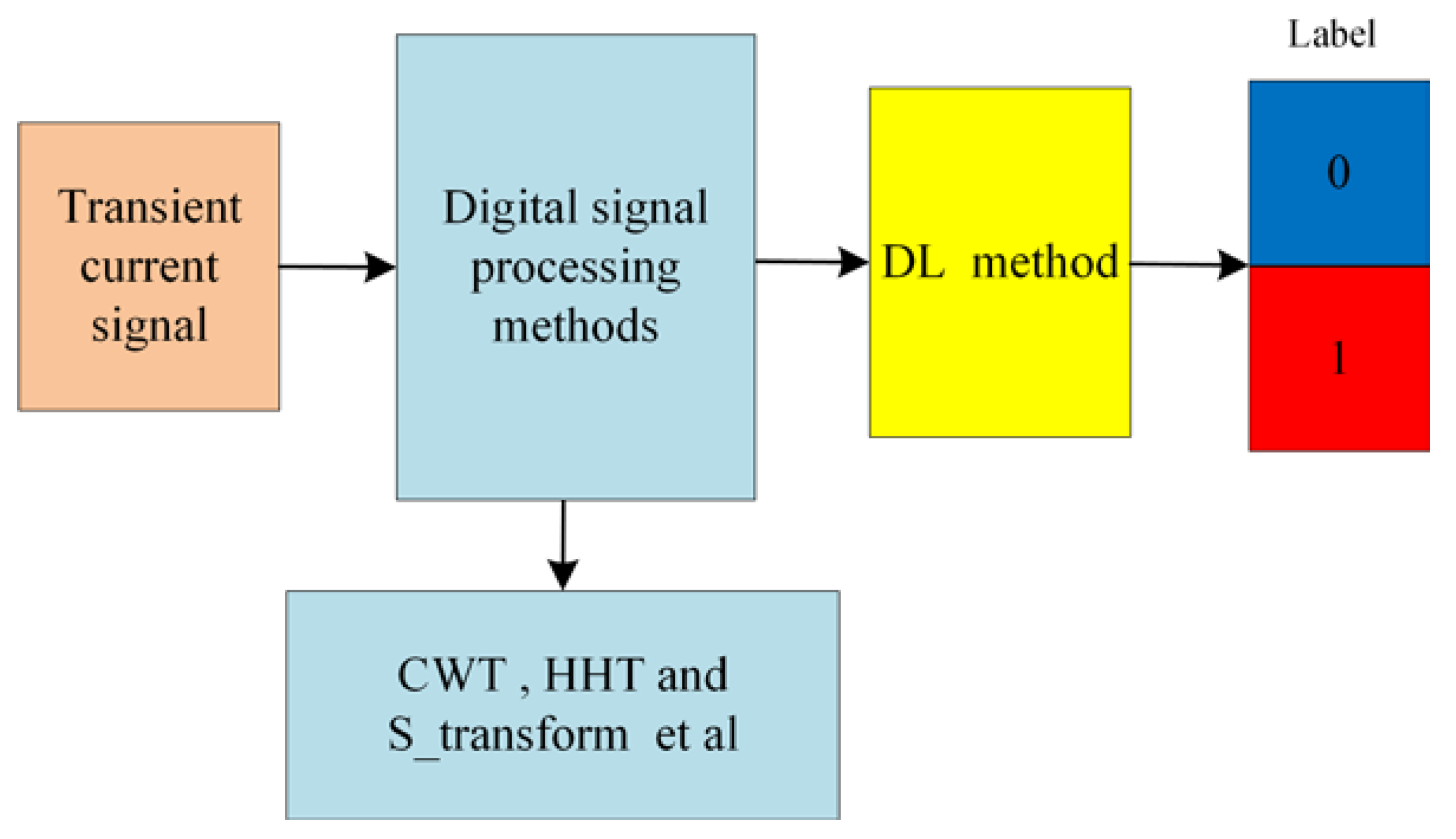
Option 2 is a digital signal processing method combined with the DL method. This method extracted the time-frequency matrix of zero-sequence current using continuous wavelet transform (CWT) [22], S-transform [23,24], HHT [25,26], and other digital signal processing methods to extract the time-frequency matrix. We input the time-frequency matrix into DL method for an adaptive extraction of fault features to complete the fault detection, as shown in Figure 2.
Guo et al. [15] obtained time-frequency grayscale images by CWT of TZSC and completed fault detection using CNN adaptive extraction of fault features. Yin et al. [23] improved the characterization of fault features by constructing S-transform correlation graphs using S-transform. Although Option 2 can improve fault detection accuracy, it still relies on digital signal processing methods for the preprocessing of raw fault data. Since the use of CWT and S-transform are mostly fixed-basis functions, Option 2 also faces the problem of insufficient fault feature characterization capability [27].

3. The Proposed Fault Detection Framework

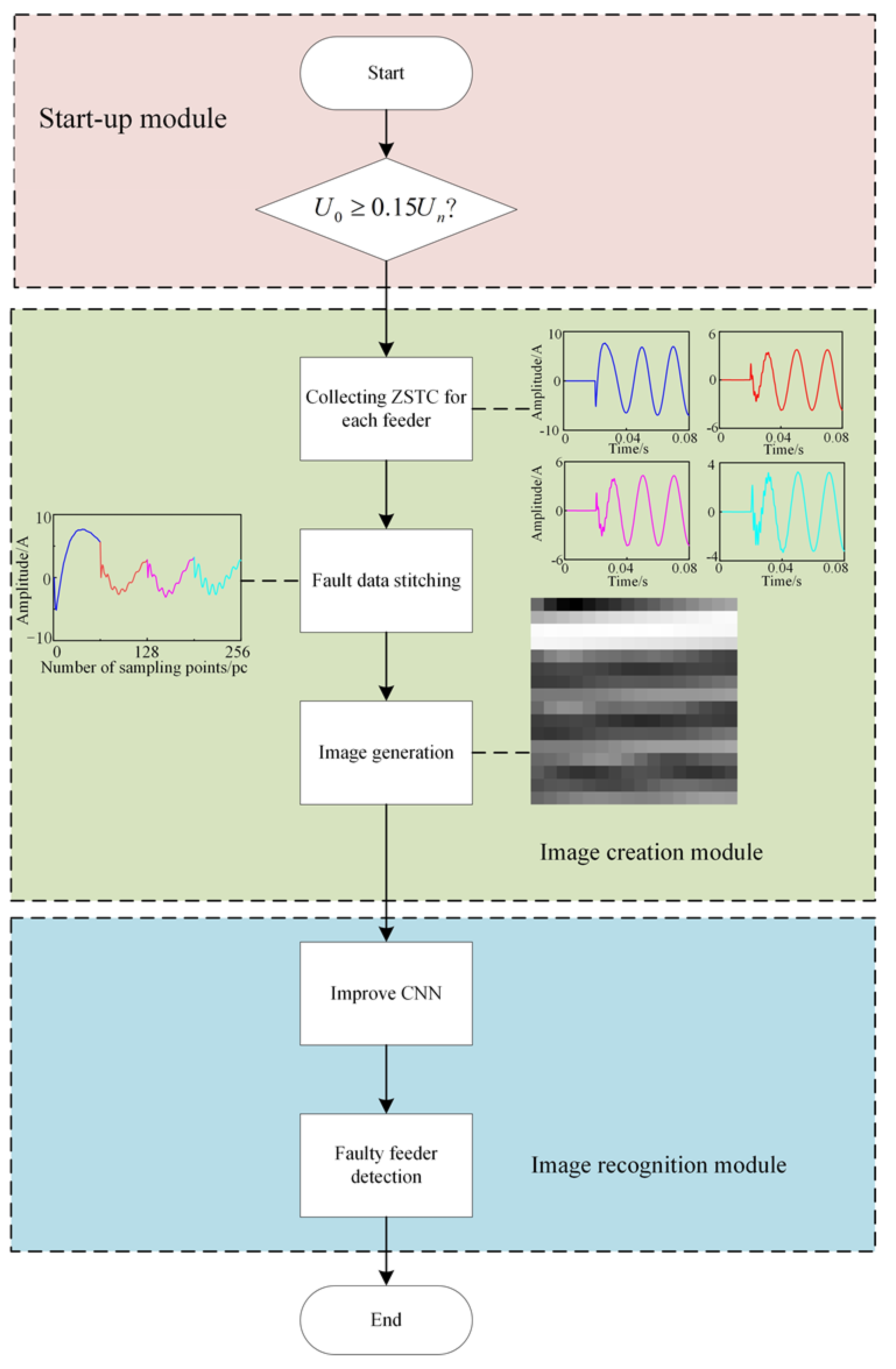
This paper proposes a fault feeder detection method based on fault data stitching and image generation, which includes three modules: (1) a startup module; (2) an image generation module; and (3) an image recognition module.
To this end, this paper proposes a fault data stitching method that considers the degree of difference between the faulty and healthy feeder TZSC under the same fault condition, which requires only simple preprocessing of the original data and has the advantage of small computational effort. The schematic diagram of the proposed method is shown in Figure 3. It is worth noting that the input samples of the proposed model in this paper are obtained by preprocessing using fault data stitching and image generation methods, rather than the digital signal processing methods mentioned in Option 1 and Option 2. In comparison, the method proposed in this paper requires only simple processing of the raw data, rather than relying on digital signal processing methods, and is less computationally intensive. The proposed method in this paper considers the differences and correlations between faulty and non-faulty feeders under the same fault conditions, which can enhance the fault characterization capability. The description of the fault characterization capability will be detailed in Section 5.
The proposed detection method can be divided into two stages: offline training and online application. In the offline training stage, a large number of historical samples are obtained by simulating the occurrence of single-phase grounding in different feeders under different fault conditions through MATLAB/SIMULINK simulation. The TZSC in the first half-cycle after the occurrence of each feeder fault is collected from the historical samples, and the TZSC of each feeder is stitched together sequentially to form the system fault data. Then the system fault data is converted into grayscale images with the signal-image conversion method, and the improved CNN is trained using a large number of fault history samples. In the online application stage, the system zero-sequence voltage and TZSC of each feeder is collected first, and when  U 0 0.15 U n  is not satisfied, it means that no single-phase ground fault occurs. When  U 0 0.15 U n  is satisfied, the collected TZSC of each feeder is stitched together and constitutes the system fault data. Finally, the system fault data are converted into grayscale images with the signal-image conversion method and input to the improved CNN model trained offline for fault feeder detection.
The fault detection method proposed in this paper has the following advantages:
(1)
It does not rely on the experience of experts and has the advantage of small computational effort.
(2)
The improved CNN identifies not the TZSC of a single feeder, but the grayscale images formed by stitching the TZSC of each feeder in a specific order, taking into account the differences and correlations between normal and faulty feeders.
(3)
The proposed fault data stitching and image generation method can enhance the characterization capability of data features.
The specific implementation will be described in detail in the next section.

4. Fault Data Stitching and Image Generation Methods

4.1. Fault Data Stitching Method

At the beginning of an SPG fault in the distribution system, the TZSC is mainly determined by the capacitance current, because the inductance current cannot change abruptly, and the sum of the TZSC currents of the healthy feeder is equal to the transient current of the faulty feeder. It can be seen that the TZSC amplitude of the faulty feeder is greater than that of the healthy feeder. Since the healthy feeder is under the same bus zero-sequence voltage, the changing trend of the TZSC waveform of the healthy feeder is the similarity. In addition, the polarity of the TZSC between the healthy feeder and the faulty feeder is opposite. For this reason, this paper proposes a fault data stitching method considering the degree of difference between the TZSC of faulty and healthy feeders under the same fault condition.
There are  k  feeders in the resonant grounding system. After the SPG fault occurs in the resonant grounding system, the TZSC of each feeder is collected and stitched according to the feeder number to obtain the system fault data, as follows.
I f = i f 1 ( 0 ) i f 2 ( 0 ) i f j ( 0 ) i f k ( 0 )
i f j ( 0 ) = ( i j ( 1 ) , i j ( 2 ) , , i j ( n ) )
where,  i f j ( 0 )  denotes the time series of the TZSC of the  j t h  feeder in half an operating frequency cycle after an SPG fault occurs in the resonant grounding system,  n  denotes the total number of TZSC sampling points in half an operating frequency cycle,   denotes the stitching operation, and  I f  denotes the system fault data generated by the stitching operation under the same fault condition. A schematic diagram of the fault data stitching method is shown in Figure 4.
As can be seen from Figure 4, the system fault data takes into account the difference and correlation between the faulty feeders and the healthy feeders and can highlight the amplitude characteristics of fault feeders. However, it is difficult to characterize the polarity of the original TZSC. Specifically, the polarity of each feeder in the system fault data takes the stitching point as the reference. Take the first feeder and the second feeder for example. The stitching point between them is the last sampling point of the first feeder. Since the amplitude of the last sampling point of the first feeder is larger than that of the first sampling point of the second feeder, the polarity direction reflected by the second feeder is downward. This is the opposite of the original polarity characteristic, as shown in Figure 5. The same is true of the stitched polarity of the other feeders. Since the amplitude relationship between the stitching point and the first sampling point of the next feeder is not guaranteed, the polarity characteristics of the feeder may be lost. For this reason, a signal-image conversion method is used in this paper to overcome the problem of the disappearance of the fault polarity characteristics caused by the stitching method. The implementation of the signal-to-image conversion method will be explained in detail in the next section.

4.2. Signal-Image Conversion Method

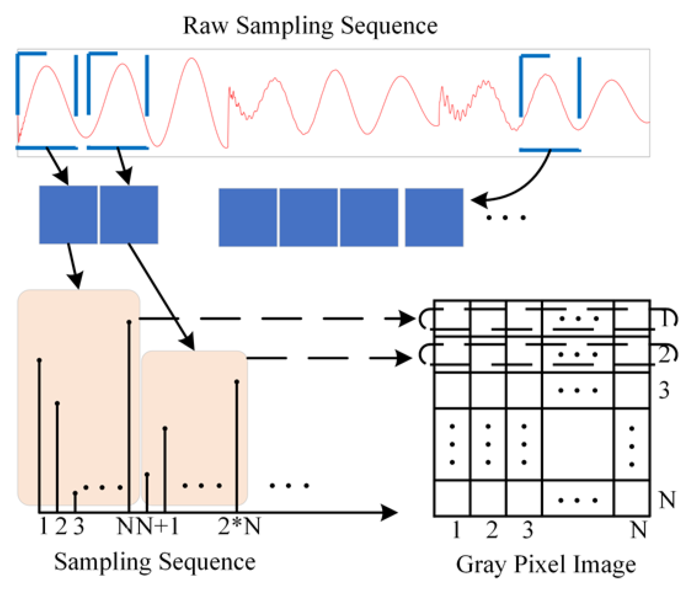
The signal-to-picture conversion method [28] is used to convert the system fault data proposed in Section 4.1 above into a two-dimensional grayscale image, the conversion method is shown in Equation (3), and the schematic diagram is shown in Figure 6.
P ( m , n ) = r o u n d ( X [ ( m 1 ) × N + n ] min ( X ) max ( X ) min ( X ) × 255 )
where  P ( m , n )  is the pixel intensity in row  m  and column  n  of the two-dimensional grayscale map;  N × N  is the size of the converted image;  X  is the value of the fault signal sequence, whose length is  N 2 X ( i )  is the value of the  i t h  data point in  X ; and  r o u n d ( · )  is used to round the data to ensure that the converted data is an integer between 0 and 255.
Taking the four-feeder system as an example, when a SPG fault occurs on feeder 1, the TZSC characteristics of the four feeders of the resonant grounding system are distributed in different regions of the grayscale image, as shown in Figure 7. It is worth noting that the pixel matrix of the fault grayscale image can express the amplitude difference of TZSC between the faulty feeder and healthy feeder under the same fault condition. There are obvious differences between the pixel values in the corresponding areas of the faulty feeder and the healthy feeder, and the pixel values in the corresponding areas of different healthy feeders have great similarities.
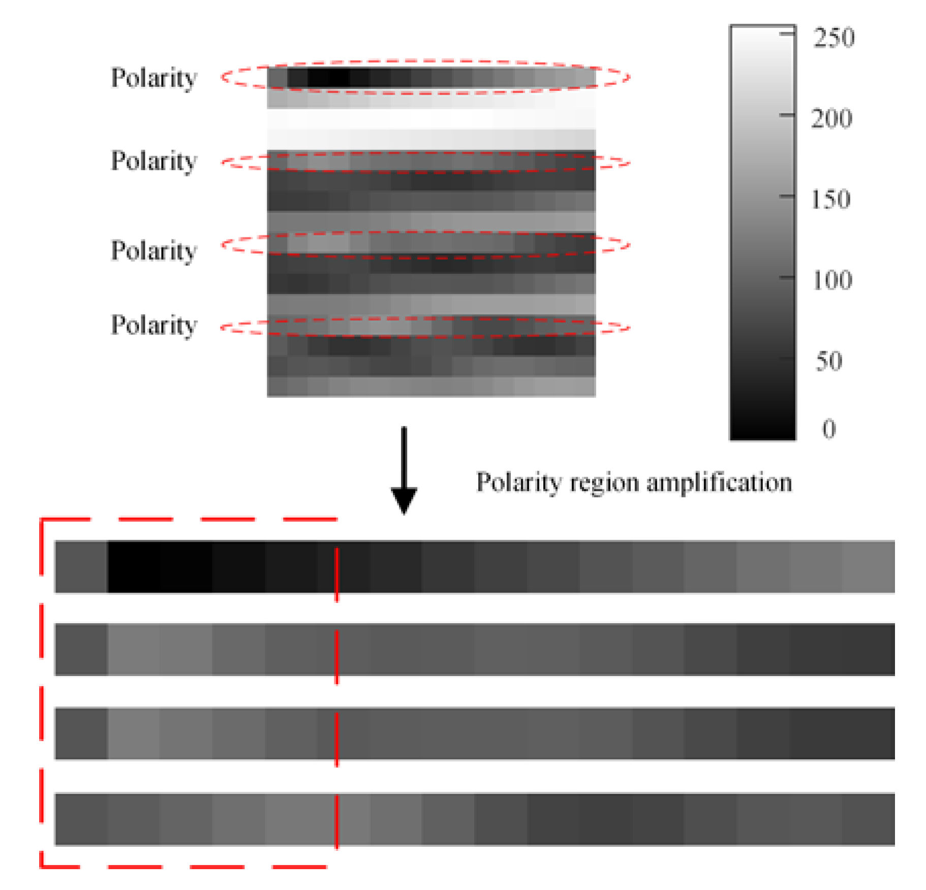
The signal-image conversion method can divide the TZSC of different feeders into different regions, which can ensure that the polarity of each feeder is based on its first sampling point. As shown in Figure 8, the part in the red box in the figure represents the distribution of the TZSC polarity characteristics of each feeder in the grayscale image. In order to better analyze the polarity distribution of the grayscale image of the system, the corresponding polarity region is enlarged. In the red box region, the color of the grayscale image corresponding to fault feeder 1 gradually becomes darker and the polarity direction is downward. The color of the grayscale image of healthy feeders 2 to 4 gradually becomes lighter and the polarity direction is upward. The polarity direction of the feeder reflected in the grayscale image is the same as that of the original TZSC. Therefore, the proposed method can preserve the polarity difference between faulty feeders and healthy feeders.
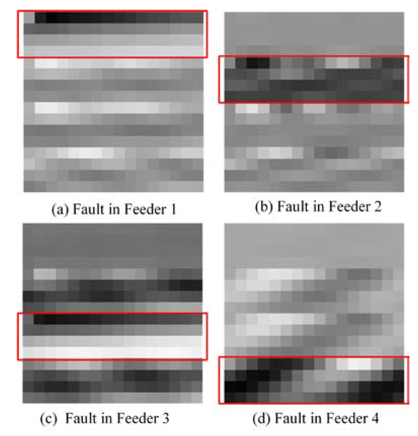
Limited by space, this paper only shows the comparison diagram of the system grayscale image corresponding to the SPG fault of four feeders, as shown in Figure 9. It can be easily seen that when SPG faults occur in different feeders, the fault features of the grayscale image of the system fault are distributed in different areas of the grayscale image with obvious differences.
To sum up, when SPG fault occurs in the distribution network system, the color of the faulty feeder region is obviously different from that of the healthy feeder region in the grayscale image of the system, and the color of healthy feeder regions is similar. In addition, the fault features of grayscale images with different feeders are distributed in different regions of grayscale images. Therefore, this feature of the grayscale image can be used for fault detection.

4.3. Fault Detection Model Based on Improved CNN

In traditional fault detection, a combination of manual feature extraction and a classifier process is usually used. However, it is not easy to achieve a proper fault feature extraction or selection. In addition, manually extracted features have a limited ability to characterize large intra-class variations. CNN is a very popular feature-learning algorithm that can exhibit good performance. Compared with traditional shallow learning models, CNN can automatically extract the features of data samples. CNN is good at local feature extraction. According to the analysis in Section 4.2, the grayscale image of the system corresponding to a SPG fault of the feeder has obvious fault characteristics in a specific area. Therefore, in this paper, CNN is used to adaptively extract the fault features of the grayscale image of the system to achieve fault detection. The proposed improved CNN in this paper borrows the LeNet-5 [29] model and makes improvements based on it: the BN layer is introduced between the convolutional and ReLu layers to accelerate the speed of CNN training and reduce the sensitivity to network initialization. The improved CNN is shown in Figure 10. The improved CNN model contains one input, three convolutional layers, two sub-sampling layers, one fully connected layer, one SoftMax, and one classification output layer.
In this paper, the input of the CNN model is the system fault grayscale image, and the output feature map of the convolutional layer (C layer) containing the BN layer is calculated as follows.
(1)
Convolution operation on the input grayscale image.
x j l = i M j x i l 1 k i j + b j l
(2)
Batch normalization of the feature map of the output after convolution using the BN algorithm [16].
x j l = γ j l x i l 1 E ( x i l 1 ) V a r ( x i l 1 ) + β j l
(3)
Activation of the batch normalized feature map, the activation function is selected as the Relu function.
x j l = f ( x i l 1 )
where  x i l 1  is the  i t h  input of the  l 1  layer.  x j l  is the  j t h  output of the  l  layer.  M j  is the set of input feature maps,  k i j  is the convolution kernel,  b j l  is the bias.  γ j l  and  β j l  are the reconstruction parameters, which can be obtained by automatic network learning.  E ( · )  is the expectation of the input samples.  V a r ( · )  is the variance of the input samples.  f ( · )  is the activation function.
The main role of the sub-sampling layer is to downsample the upper layer input feature maps while preventing data overfitting. This paper uses average pooling, calculated as
x j l = f m e a n ( i M j x i l 1 + b j l )
where,  f m e a n  is the mean value function.
The Softmax layer maps the feature vector output from the fully connected layer to the sample labeling space to obtain a new feature expression form and calculates the probability of each type corresponding to the current sample as
P ( y = i | z ) = exp ( z i ) i exp ( z i )
where  z  is the input of the fully connected layer and  P ( y = i | z )  is the probability value of the  i t h  category.
The training process of CNN includes forward propagation and back propagation. After the weight and bias of the convolutional neural network are initialized, a large number of grayscale images of system faults can be used to train the improved CNN. After multiple backpropagations to adjust the kernel parameters, a CNN model with fault feeder detection ability can be trained. This paper proposes the relevant parameters of the improved CNN model as shown in Table 1. The optimization solver for improved CNN model is the SGDM algorithm, the MiniBatchSize is 128, and an initial learning rate is 0.01.

5. Example Analysis

The experiments in this paper are run on Windows 10 with a computer configuration of Inter Core i7-10400F CPU, 2.5 GHz, 4 GB of RAM, GTX 1050Ti GPU, and MATLAB R2020a programming software.

5.1. Simulation Model Building

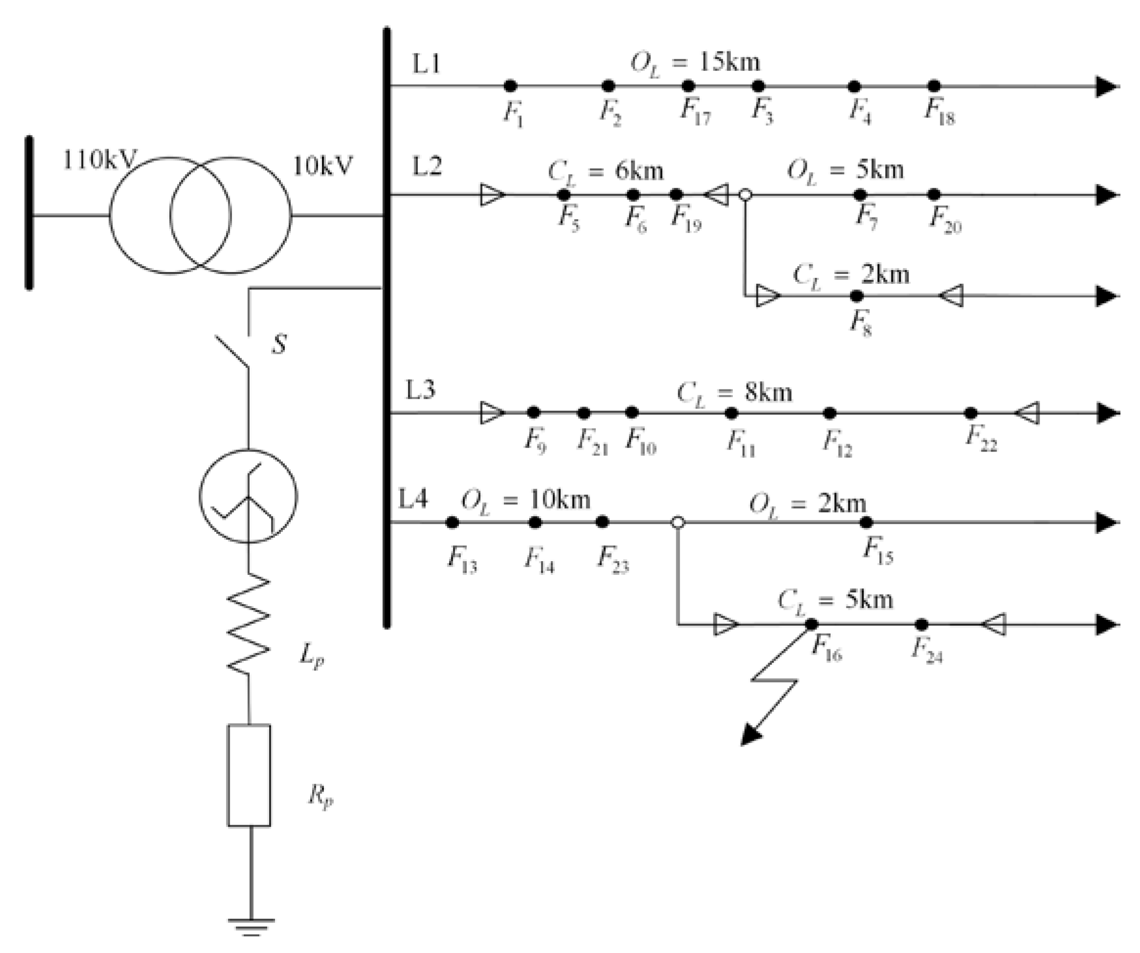
In this paper, the resonant grounding distribution system was built on MATLAB/SIMULINK, and the simulation model is shown in Figure 11. Where  O L  denotes the overhead line length,  C L  denotes the cable line length. The line impedance parameters [15] are shown in Table 2. The arc extinguishing coil compensation degree is 5%, and the sampling rate is 6.4 kHz.

5.2. Fault Dataset Generation

To obtain the fault data samples, the grid voltage, ground resistance, initial fault angle, and fault distance were simulated separately, and the training samples and test samples simulation parameters are traversed in the table, as shown in Table 3.

5.3. Fault Characterization Capability Analysis

To verify that the fault data stitching and image generation methods proposed in Section 3 of this paper enhanced the characterization of the raw data fault features, the training samples data were processed and visualized using the T-SNE algorithm [30] for this paper in the following two ways:
(1)
Direct visualization of the fault feeder data from the training samples;
(2)
Pre-processing the training samples using the proposed fault stitching and image generation methods, followed by visualization.
The results of the two visualization methods are shown in Figure 12, and legends numbered 1 to 4 in Figure 12 indicate the number of feeders where grounding faults occurred.
As can be seen from Figure 12, the proposed method considers the connection between healthy and faulty feeders under the same fault condition, which enhances the characterization of data fault features.
In summary, the grayscale images obtained by processing the TZSC of each feeder through fault data stitching and image generation methods have the following advantages:
(1)
The ability to preserve the difference between healthy and faulty feeders;
(2)
The converted grayscale image can retain the amplitude features and polarity features of the faulty feeder and the healthy feeder;
(3)
The method can fix the fault features in a specific region, enhancing the feature characterization of the system’s grayscale images.

5.4. Model Training and Testing

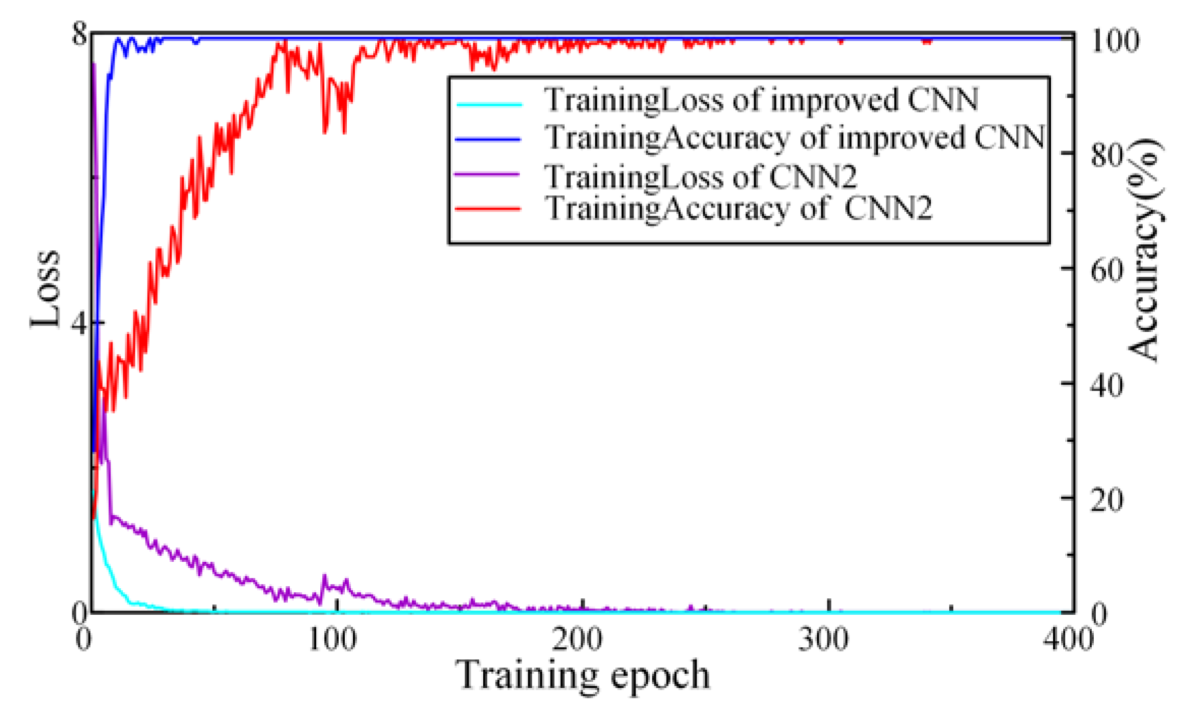
The improved CNN was trained using 5760 samples from the training samples to generate 5760 two-dimensional grayscale images, according to the method proposed in this paper. As a comparison, the BN layer between the convolutional and activation layers was removed based on the proposed improved CNN model to obtain the new CNN model, which we named CNN2. The loss function value curves and the detection accuracy curves for the convergence of the improved CNN and CNN2 training iterations are shown in Figure 13. The improved CNN and CNN2 training process took a total of 400 iterations and 47 s. After 49 iterations, the correct fault detection rate reached 100% and the value of the loss function decreased to 0.0089, while the correct detection rate reached 100% and the value of the loss function decreased to 0.0121 after 306 iterations of CNN2. This shows that adding a BN layer can accelerate the training speed of the model.
By changing the parameters of the simulation model in Table 3, the simulation generated 720 samples of fault data that were different from the above training process and generated two-dimensional grayscale images as the test set of the model. The fault selection accuracy of the proposed method and CNN2 both reached 100%.

5.5. Comparison of Algorithms

To verify the effectiveness of the proposed method in this paper, four methods of fault routing based on TZSC were selected for comparison. The related methods are described as follows:
(1)
Model-1
Model-1 uses manual feature extraction combined with SVM [15], where the optimal penalty factor  C = 1  and kernel function parameters  σ = 0 . 3125  of SVM are obtained with the cross-validation method.
(2)
Model-2
Model-2 uses WT [31] combined with CNN, and the db5 wavelet is selected as the wavelet basis function.
(3)
Model-3
Model-3 uses the one-dimensional signal-based CNN (1D-CNN) feeder detection method [23].
(4)
Model-4
Model-4 took as input the normalized system fault data generated by the fault data stitching method described in Section 2.1, the model used the deep belief network (DBN) [32] model optimized by Spider Monkey Optimization [33] (SMO), and the optimized number of nodes in the implicit layer is [66,73,157].

5.5.1. Comparison of Different Models

To verify the effectiveness of the proposed method, it was compared with Model-1, Model-2, Model-3 and Model-4, and the test results of different methods are shown in Table 4.
Among them, the proposed method in this paper was 5.42% more accurate than Method-4 in terms of feeder detection, indicating that the conversion of system fault data into grayscale images can enhance the characterization of fault features, which in turn ensures the accuracy of fault detection.

5.5.2. Robustness Comparison of Models

To verify the robustness of the model, the effects of system operation changes, reverse installation of zero-sequence current transformers, noise, and sampling delay on the detection accuracy of the model were considered separately. The method described in Section 5.5 and the proposed method in this paper were used for comparison.
(1)
Change of neutral-point operation mode
As shown in Figure 9, the switch S was opened and the system was changed to a neutral ungrounded system. Then, 288 test samples were obtained by changing the fault operation parameters, and the test results of different methods are shown in Table 5.
From Table 4 and Table 5, it can be seen that the proposed method can be well adapted to neutral ungrounded system faults, as long as the network structure does not change and only the neutral grounding method is changed. The fault detection method based on this paper can accurately detect the faulty feeder without retraining the model.
(2)
Reverse installation of CTs
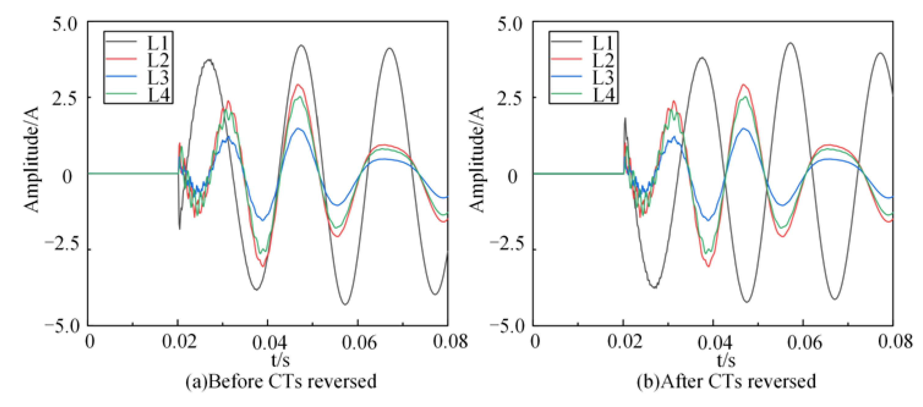
In the actual power system, sometimes the reverse installation of the zero-sequence current transformers (CTs) due to human error can lead to a change in the polarity of the original TZSC, which will increase the difficulty of fault detection. To simulate the actual power system, this paper sets 40% of the faulty feeders to have reverse installations of CTs. The distribution of test data is shown in Table 6.
To demonstrate the fault waveform situation when the CTs are reversed and set up a single-phase ground fault on Feeder 1, Figure 14a shows the zero-sequence current waveform before the CTs were reversed and installed on Feeder 1, and Figure 14b shows the zero-sequence current waveform after the CTs were reversed and installed on Feeder 1. From Figure 14, it can be seen that the polarity characteristics of the faulty Feeder 1 have disappeared after the reversed installation of CTs, leaving only the information on amplitude characteristics.
The test data after CT reversal was tested and the test results of different methods are shown in Table 7.
From Table 4 and Table 7, it can be seen that Model-2 adopted WT transform to extract the time-frequency features of TZSC and can well avoid the influence brought by CT reverse installations, so the correct rate of line selection remains unchanged, and the 1D-CNN timing matrix in Model-3 was susceptible to the influence of CT reverse installations, which lead to the change, offset or misalignment of fault feeder detection features [34], and thus the feeder detection accuracy decreased. Model-4 is susceptible to CT reversal installations, which lead to degradation of the routing accuracy. The performance of the proposed method is better than that of Model-1 to Model-4. Because the proposed method can retain the amplitude and polarity characteristics of the faulty and normal feeders; even when the polarity characteristics disappear, the existence of the amplitude characteristics can ensure the correctness of the detection.
(3)
Noise impact
Since the detection results are susceptible to noise degradation, to verify the anti-interference ability of the proposed algorithm, 720 samples of data used in the test were superimposed with Gaussian white noise of different signal-to-noise ratios (SNR), and all models were run 10 times to take the average detection accuracy as the evaluation index. The average fault detection accuracy of different methods after superimposing noise on the test set is shown in Figure 15.
As can be seen from Figure 15, the average detection accuracy of Model-1 to Model-3 decreased as the SNR decreased, while the average detection accuracy of the proposed method is 100% when the SNR was greater than 10dB, and the average correct detection rate was 99.92% when the SNR was equal to 10dB. It shows that the proposed method has strong anti-noise capability.
(4)
Sampling delay
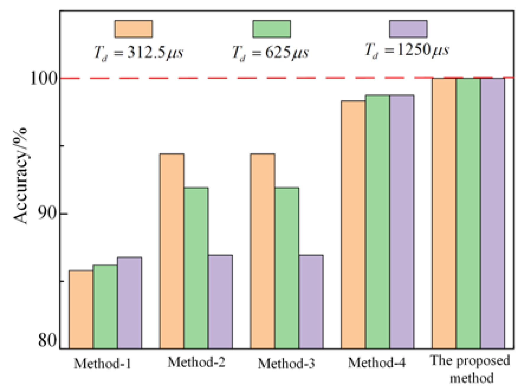
Due to the actual situation, the zero-sequence sampling time of each feeder is difficult to absolutely synchronize, so the sampling delay was simulated. The sampling time difference of feeders L1–L2 and L3–L4 was set to simulate the scenario of asynchronous sampling delay in each feeder. Sample delay test results are shown in Figure 16.
As can be seen from Figure 16, when a sampling delay occurred, the feeder detection accuracy of the proposed method was maintained at 100%, which is superior to other DL methods and ML methods. This shows that the proposed method has good robustness.
(5)
Sampling delay
In actual engineering, the sampling time of the TZSC of each feeder is difficult to absolutely synchronize and is easily disturbed by noise. To verify the effectiveness of the proposed method, in the 720 samples of data in Section 5.2, the sampling delay was set for feeders L1 to L2 and L3 to L4, and the delay time was 1250  μ s . On this basis, noise with SNR of 10dB was superimposed, which generated the data set with asynchronous noise sampling. The above four comparison methods were repeated 10 times, and the results of different methods of feeder detection are shown in Table 8.
As can be seen from Table 8, the average line selection accuracy of the proposed method is 99.51% in the presence of Gaussian white noise with asynchronous sampling delay, which indicates that the proposed method has good robustness.

6. Conclusions

This paper proposes a resonant ground fault detection method based on fault data stitching and image generation. The following conclusions were obtained.
(1)
The proposed fault data stitching method can highlight the amplitude characteristics of the faulty feeder. Secondly, the signal-image conversion method is used to make up for the possible fault polarity confusion in the fault data stitching method. Finally, the visualization technique is used to verify that the proposed fault data stitching and image generation methods can enhance the characterization ability of fault features.
(2)
The improved CNN model can accelerate the training speed of the model, the model is not easily affected by fault conditions, and has high detection accuracy.
(3)
Compared with existing detection methods, the proposed improved CNN fault line selection model shows superior robustness and good adaptability under the conditions of neutral operation mode change, noise, CT reversal and sampling delay.
The method proposed in this paper takes the simulation data as the experimental sample and obtains high detection accuracy. Considering the difference between actual distribution network data and simulation data, the next research direction will add fault data from the actual power network to further improve the fault detection model and improve the practicability of the method. Secondly, in view of the poor interpretability of the model, the next step is to introduce SE (Squeeze-and-Excitation), CBAM (Convolutional Block Attention Module) and other interpretability methods to enhance the interpretability of the model.

Author Contributions

Methodology, X.N., J.Z., Y.H., W.L., T.G. and B.L.; Software, X.N. and W.L.; Validation, X.N., T.G. and B.L.; Resources, J.Z. and Y.H.; Writing—original draft, X.N. and X.H.; Writing—review & editing, J.Z., Y.H., T.G., B.L. and X.H.; Visualization, W.L. and X.H.; Supervision, J.Z. and Y.H.; Project administration, Y.H.; Funding acquisition, J.Z. and Y.H. All authors have read and agreed to the published version of the manuscript.

Funding

This work was supported by National Natural Science Foundation of China (NSFC) (No.51867005), The Science and Technology Foundation of Guizhou Province ([2022] general013, [2022] general014), The Science and Technology Foundation of Guizhou Province (GCC [2022]016-1), Educational Technology Foundation of Guizhou Province ([2022]043).

Data Availability Statement

Not applicable.

Conflicts of Interest

The authors declare no conflict of interest.

References

  1. Wang, X.; Gao, J.; Song, G.; Cheng, Q.; Wei, X.; Wei, Y. Faulty Line Selection Method for Distribution Network Based on Variable Scale Bistable System. J. Sens. 2016, 2016, 7436841. [Google Scholar] [CrossRef] [Green Version]
  2. Shafiullah, M.; Abido, M.A. S-Transform Based FFNN Approach for Distribution Grids Fault Detection and Classification. IEEE Access 2018, 6, 8080–8088. [Google Scholar] [CrossRef]
  3. Wang, Y.; Huang, Y.; Zeng, X.; Wei, G.; Zhou, J.; Fang, T.; Chen, H. Faulty Feeder Detection of Single Phase-Earth Fault Using Grey Relation Degree in Resonant Grounding System. IEEE Trans. Power Deliv. 2017, 32, 55–61. [Google Scholar] [CrossRef]
  4. Li, Z.; Ye, Y.; Ma, X.; Lin, X.; Xu, F.; Wang, C.; Ni, X.; Ding, C. Single-Phase-to-Ground Fault Section Location in Flexible Resonant Grounding Distribution Networks Using Soft Open Points. Int. J. Electr. Power Energy Syst. 2020, 122, 106198. [Google Scholar] [CrossRef]
  5. Jin, N.; Xing, J.; Liu, Y.; Li, Z.; Lin, X. A Novel Single-Phase-to-Ground Fault Identification and Isolation Strategy in Wind Farm Collector Line. Int. J. Electr. Power Energy Syst. 2018, 94, 15–26. [Google Scholar] [CrossRef]
  6. Wang, B.; Geng, J.; Dong, X. High-Impedance Fault Detection Based on Nonlinear Voltage–Current Characteristic Profile Identification. IEEE Trans. Smart Grid 2018, 9, 3783–3791. [Google Scholar] [CrossRef]
  7. Yuan, J.; Jiao, Z.; Feng, G.; Chen, M.; Xu, M. Study on Fault Line Detection Methods Based on Multi-feature Fusion in Distribution Systems. IET Gener. Transm. Distrib. 2021, 15, 860–869. [Google Scholar] [CrossRef]
  8. Namdari, F.; Salehi, M. High-Speed Protection Scheme Based on Initial Current Traveling Wave for Transmission Lines Employing Mathematical Morphology. IEEE Trans. Power Deliv. 2017, 32, 246–253. [Google Scholar] [CrossRef]
  9. Xie, L.; Luo, L.; Li, Y.; Zhang, Y.; Cao, Y. A Traveling Wave-Based Fault Location Method Employing VMD-TEO for Distribution Network. IEEE Trans. Power Deliv. 2020, 35, 1987–1998. [Google Scholar] [CrossRef]
  10. Yuan, J.; Jiao, Z. Faulty Feeder Detection Based on Fully Convolutional Network and Fault Trust Degree Estimation in Distribution Networks. Int. J. Electr. Power Energy Syst. 2022, 141, 108264. [Google Scholar] [CrossRef]
  11. Ghaderi, A.; Mohammadpour, H.A.; Ginn, H.L.; Shin, Y.-J. High-Impedance Fault Detection in the Distribution Network Using the Time-Frequency-Based Algorithm. IEEE Trans. Power Deliv. 2015, 30, 1260–1268. [Google Scholar] [CrossRef]
  12. Sahani, M.; Dash, P.K. Fault Location Estimation for Series-Compensated Double-Circuit Transmission Line Using Parameter Optimized Variational Mode Decomposition and Weighted P-Norm Random Vector Functional Link Network. Appl. Soft Comput. 2019, 85, 105860. [Google Scholar] [CrossRef]
  13. Guo, M.-F.; Yang, N.-C.; Chen, W.-F. Deep-Learning-Based Fault Classification Using Hilbert–Huang Transform and Convolutional Neural Network in Power Distribution Systems. IEEE Sens. J. 2019, 19, 6905–6913. [Google Scholar] [CrossRef]
  14. Wang, X.; Zhou, P.; Peng, X.; Wu, Z.; Yuan, H. Fault Location of Transmission Line Based on CNN-LSTM Double-Ended Combined Model. Energy Rep. 2022, 8, 781–791. [Google Scholar] [CrossRef]
  15. Guo, M.-F.; Zeng, X.-D.; Chen, D.-Y.; Yang, N.-C. Deep-Learning-Based Earth Fault Detection Using Continuous Wavelet Transform and Convolutional Neural Network in Resonant Grounding Distribution Systems. IEEE Sens. J. 2018, 18, 1291–1300. [Google Scholar] [CrossRef]
  16. Yuan, J.; Jiao, Z. Faulty Feeder Detection Based on Image Recognition of Current Waveform Superposition in Distribution Networks. Appl. Soft Comput. 2022, 130, 109663. [Google Scholar] [CrossRef]
  17. Wei, X.; Yang, D.; Wang, X.; Wang, B.; Gao, J.; Wei, K. Faulty Feeder Detection Based on Fundamental Component Shift and Multiple-Transient-Feature Fusion in Distribution Networks. IEEE Trans. Smart Grid 2021, 12, 1699–1711. [Google Scholar] [CrossRef]
  18. Ince, T.; Kiranyaz, S.; Eren, L.; Askar, M.; Gabbouj, M. Real-Time Motor Fault Detection by 1-D Convolutional Neural Networks. IEEE Trans. Ind. Electron. 2016, 63, 7067–7075. [Google Scholar] [CrossRef]
  19. Ioffe, S.; Szegedy, C. Batch Normalization: Accelerating Deep Network Training by Reducing Internal Covariate Shift. arXiv 2015, arXiv:1502.03167. [Google Scholar]
  20. Zhang, J.; He, Z.Y.; Lin, S.; Zhang, Y.B.; Qian, Q.Q. An ANFIS-Based Fault Classification Approach in Power Distribution System. Int. J. Electr. Power Energy Syst. 2013, 49, 243–252. [Google Scholar] [CrossRef]
  21. Adewole, A.C.; Tzoneva, R.; Behardien, S. Distribution Network Fault Section Identification and Fault Location Using Wavelet Entropy and Neural Networks. Appl. Soft Comput. 2016, 46, 296–306. [Google Scholar] [CrossRef]
  22. Liang, P.; Wang, W.; Yuan, X.; Liu, S.; Zhang, L.; Cheng, Y. Intelligent Fault Diagnosis of Rolling Bearing Based on Wavelet Transform and Improved ResNet under Noisy Labels and Environment. Eng. Appl. Artif. Intell. 2022, 115, 105269. [Google Scholar] [CrossRef]
  23. Yin, H.; Miao, S.; Guo, S. Novel Method for Single-Phase Grounding Fault Line Selection in Distribution Network Based on S-Transform Correlation and Deep Learning. Electr. Power Autom. Equip. 2021, 41, 88–96. [Google Scholar]
  24. Chavez, J.J.; Popov, M.; López, D.; Azizi, S.; Terzija, V. S-Transform Based Fault Detection Algorithm for Enhancing Distance Protection Performance. Int. J. Electr. Power Energy Syst. 2021, 130, 106966. [Google Scholar] [CrossRef]
  25. Zhu, X.; Li, S.; Guo, Y.; Chen, X.; He, C.; Deng, J. Novel Wavefront Detection and Fault Location Method Based on Hilbert-Huang Transform for Long HVDC Transmission Lines. Electr. Power Syst. Res. 2022, 211, 108213. [Google Scholar] [CrossRef]
  26. Shamlou, A.; Feyzi, M.R.; Behjat, V. Winding Deformation Classification in a Power Transformer Based on the Time-Frequency Image of Frequency Response Analysis Using Hilbert-Huang Transform and Evidence Theory. Int. J. Electr. Power Energy Syst. 2021, 129, 106854. [Google Scholar] [CrossRef]
  27. Wang, X.; Gao, J.; Wei, X.; Song, G.; Wu, L.; Liu, J.; Zeng, Z.; Kheshti, M. High Impedance Fault Detection Method Based on Variational Mode Decomposition and Teager–Kaiser Energy Operators for Distribution Network. IEEE Trans. Smart Grid 2019, 10, 6041–6054. [Google Scholar] [CrossRef]
  28. Wen, L.; Li, X.; Gao, L.; Zhang, Y. A New Convolutional Neural Network-Based Data-Driven Fault Diagnosis Method. IEEE Trans. Ind. Electron. 2018, 65, 5990–5998. [Google Scholar] [CrossRef]
  29. Nguyen-Duc, T.; Le-Viet, T.; Nguyen-Dang, D.; Dao-Quang, T.; Bui-Quang, M. Photovoltaic Array Reconfiguration under Partial Shading Conditions Based on Short-Circuit Current Estimated by Convolutional Neural Network. Energies 2022, 15, 6341. [Google Scholar] [CrossRef]
  30. Zhan, X.; Han, S.; Rong, N.; Liu, P.; Ao, W. A Two-Stage Transient Stability Prediction Method Using Convolutional Residual Memory Network and Gated Recurrent Unit. Int. J. Electr. Power Energy Syst. 2022, 138, 107973. [Google Scholar] [CrossRef]
  31. Hao, S.; Zhang, X.; Ma, R. Fault Line Selection Method for Small Current Grounding System Based on Improved GoogLeNet. Power Syst. Technol. 2022, 46, 361–368. [Google Scholar]
  32. Shao, H.; Jiang, H.; Zhang, X.; Niu, M. Rolling Bearing Fault Diagnosis Using an Optimization Deep Belief Network. Meas. Sci. Technol. 2015, 26, 115002. [Google Scholar] [CrossRef]
  33. Gui, T.; Ma, C.; Wang, F.; Jinyang, L.; Wilkins, D.E. A Novel Cluster-Based Routing Protocol Wireless Sensor Networks Using Spider Monkey Optimization. In Proceedings of the IECON 2016–42nd Annual Conference of the IEEE Industrial Electronics Society, Florence, Italy, 23–26 October 2016; pp. 5657–5662. [Google Scholar]
  34. Du, Y.; Liu, Y.; Shao, Q.; Luo, L.; Dai, J.; Sheng, G.; Jiang, X. Single Line-to-Ground Faulted Line Detection of Distribution Systems With Resonant Grounding Based on Feature Fusion Framework. IEEE Trans. Power Deliv. 2019, 34, 1766–1775. [Google Scholar] [CrossRef]
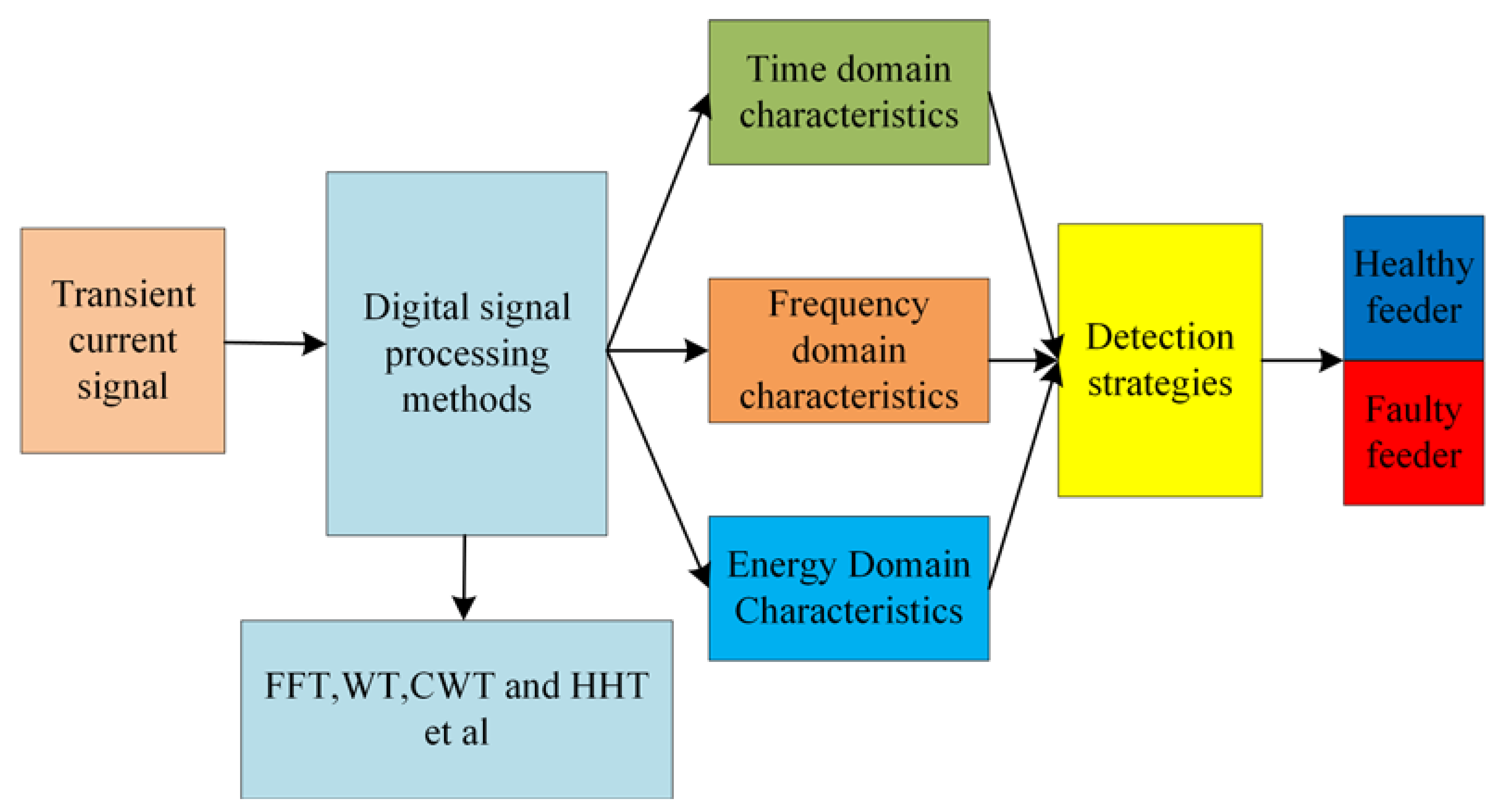
Figure 1. Flow chart of Option 1. If it is a faulty feeder, the output label is ‘1’; otherwise, the output label is ‘0’.
Energies 16 02937 g001
Figure 2. Flow chart of Option 2. If it is a faulty feeder, the output label is ‘1’; otherwise, the output label is ‘0’.
Energies 16 02937 g002
Figure 3. Proposed fault detection framework.
Energies 16 02937 g003
Figure 4. Fault data stitching method.
Energies 16 02937 g004
Figure 5. Schematic diagram of system fault data polarity analysis.
Energies 16 02937 g005
Figure 6. Signal-image conversion method.
Energies 16 02937 g006
Figure 7. System failure grayscale image feature analysis diagram. The darker the color of the pixel in the graph, the smaller the corresponding TZSC sampling value. The lighter the color of the pixel in the graph, the larger the corresponding TZSC sampling value.
Energies 16 02937 g007
Figure 8. Polarity feature analysis diagram of grayscale image of system fault.
Energies 16 02937 g008
Figure 9. Grayscale images of the system with different feeder faults.
Energies 16 02937 g009
Figure 10. Improved CNN model diagram.
Energies 16 02937 g010
Figure 11. Resonant grounding distribution system model.
Energies 16 02937 g011
Figure 12. Different ways to visualize.
Energies 16 02937 g012
Figure 13. Two model training iteration curves.
Energies 16 02937 g013
Figure 14. Ground fault on Feeder 1 ( 0 ,   5   km ,   2000 Ω ) .
Energies 16 02937 g014
Figure 15. Test results of different methods under different noise intensity.
Energies 16 02937 g015
Figure 16. Test results of different methods undersampling delay.
Energies 16 02937 g016
Table 1. Layer configurations of CNN model.
Layer TypesOutput Feature SizeConvolution Kernel Size-NumberStrideActivation Function
Input   16 × 16 × 1
C1   16 × 16 × 32   8 × 8 1Relu
S1   7 × 7 × 32   4 × 4 2
C2   7 × 7 × 16   4 × 4 1Relu
S2   3 × 3 × 16   2 × 2 2
C3   3 × 3 × 8   4 × 4 1Relu
FC layer   72 × 1
Output   4 × 1
Table 2. Line impedance parameters.
Line TypesSequenceResistance
( Ω / km )
Inductance
( m H / km )
Capacitance
( μ F / km )
OverheadPositive-sequence0.1251.30.0096
Zero-sequence0.2754.60.0054
CablePositive-sequence0.270.2550.339
Zero-sequence2.71.0190.28
Table 3. Simulation parameter traversal table.
ParametersValueSample Size
Training
samples
Voltage/kV9.5, 10.0, 10.55760
Fault TypeA-G, B-G, C-G
Fault phase angle/degree0, 30, 45, 60, 90
Transition Resistors/ Ω  1, 50, 100, 200, 500, 1000, 1500, 2000
Fault distanceIn Figure 11 F 1 F 16  
Testing
samples
Voltage/kV10.0720
Fault TypeA-G, B-G, C-G
Fault phase angle degree20, 40, 50, 70, 80
Transition Resistors/ Ω  10, 300, 800, 1200, 2000, 3000
Fault distanceIn Figure 11 F 17 F 24  
Table 4. Feeder detection results of different methods.
Feeder Detection MethodModel-1Model-2Model-3Model-4The Proposed Method
Accuracy/%84.2495.6310094.58100
Table 5. Test results of an ungrounded system.
MethodModel-1Model-2Model-3Model-4The Proposed Method
Accuracy/%67.1979.8681.2580.21100
Table 6. Test data distribution table for CTs with reversed connections.
Fault TypeThe Number of Samples with Reversed CTs in Testing DataThe Number of Samples with Correct CTs in Testing DataThe Number of Testing Data
Fault in Feeder 172108180
Fault in Feeder 272108180
Fault in Feeder 372108180
Fault in Feeder 472108180
Table 7. Test result of reversed CTs.
MethodModel-1Model-2Model-3Model-4The Proposed Method
Accuracy/%84.7295.6393.6180.56100
Table 8. Feeder detection results of different methods of superimposing 10 dB noise under asynchronous delay.
MethodModel-1Model-2Model-3Model-4The Proposed Method
Average accuracy/%7085.3394.5197.0799.51
Disclaimer/Publisher’s Note: The statements, opinions and data contained in all publications are solely those of the individual author(s) and contributor(s) and not of MDPI and/or the editor(s). MDPI and/or the editor(s) disclaim responsibility for any injury to people or property resulting from any ideas, methods, instructions or products referred to in the content.