
An Improved Method to Accurately Estimate TOC of Shale Reservoirs and Coal-Measures

Abstract
:1. Introduction
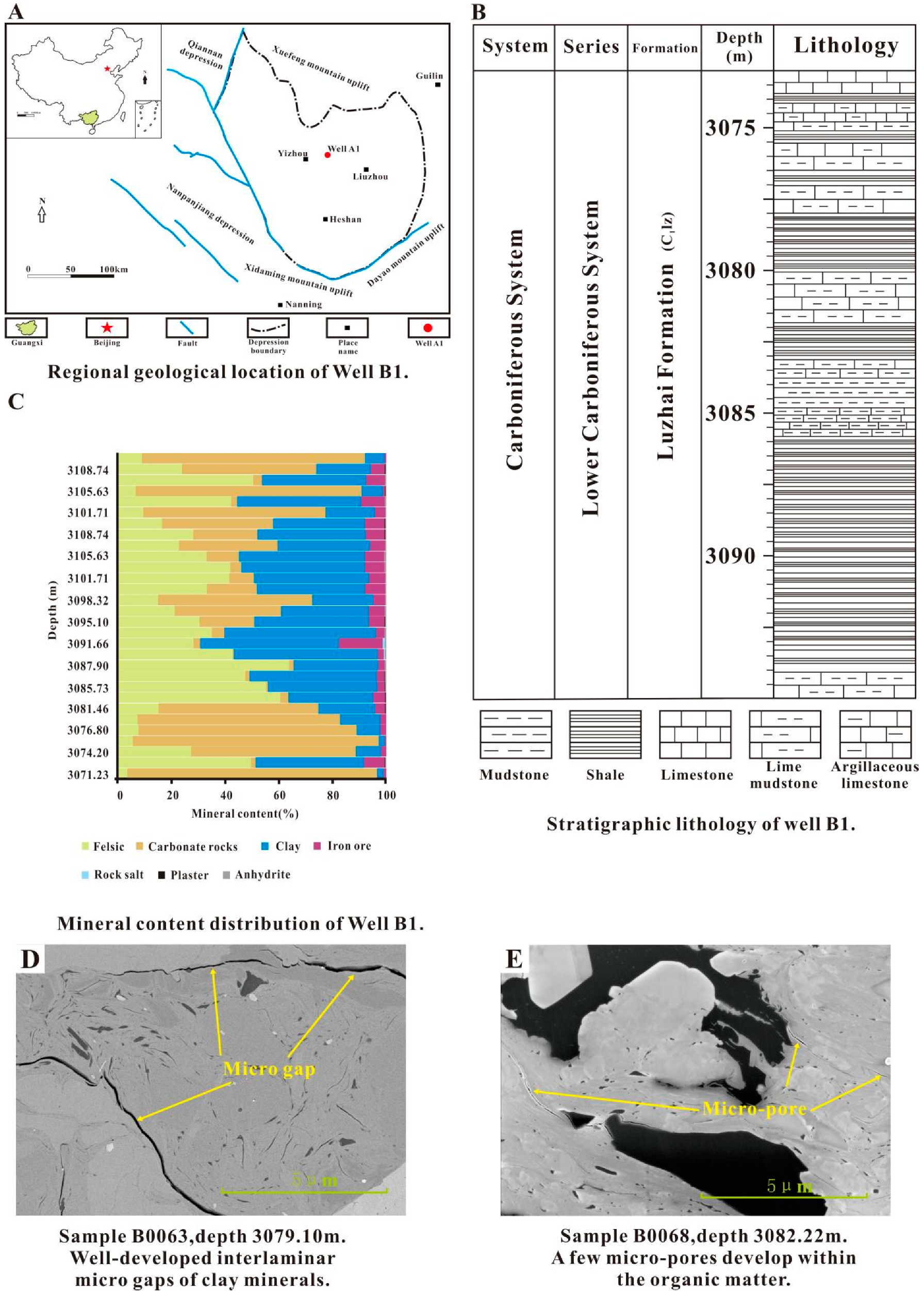
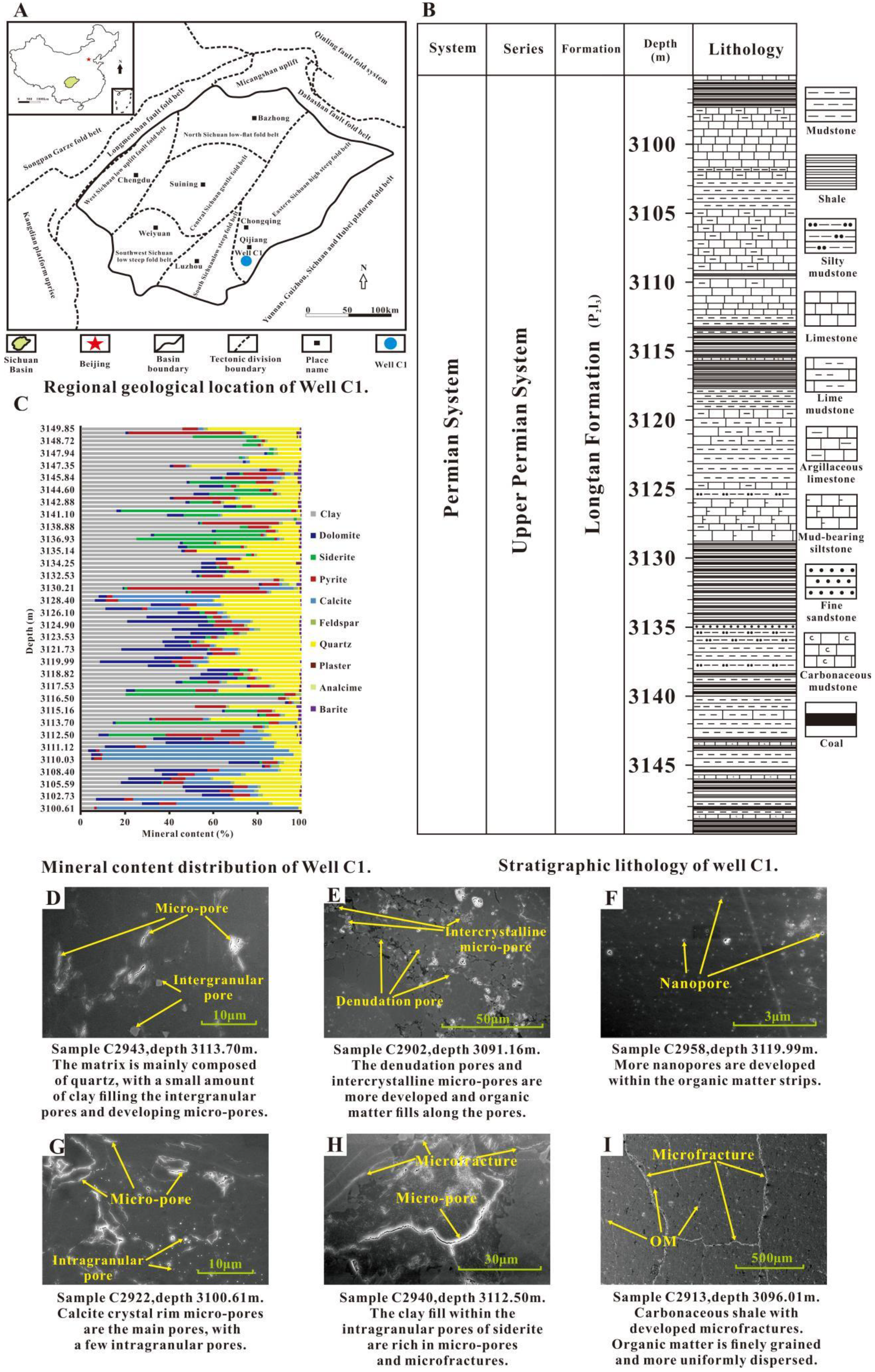
2. Geological Background
3. Theory and Method
3.1. ∆log R Method
- (1)
- Scale porosity and resistivity curves
- (2)
- Determine a suitable baseline
- (3)
- Calculate each baseline value
3.2. Overlapping Shapes of Sonic and Resistivity Curves and Reservoir Parameters
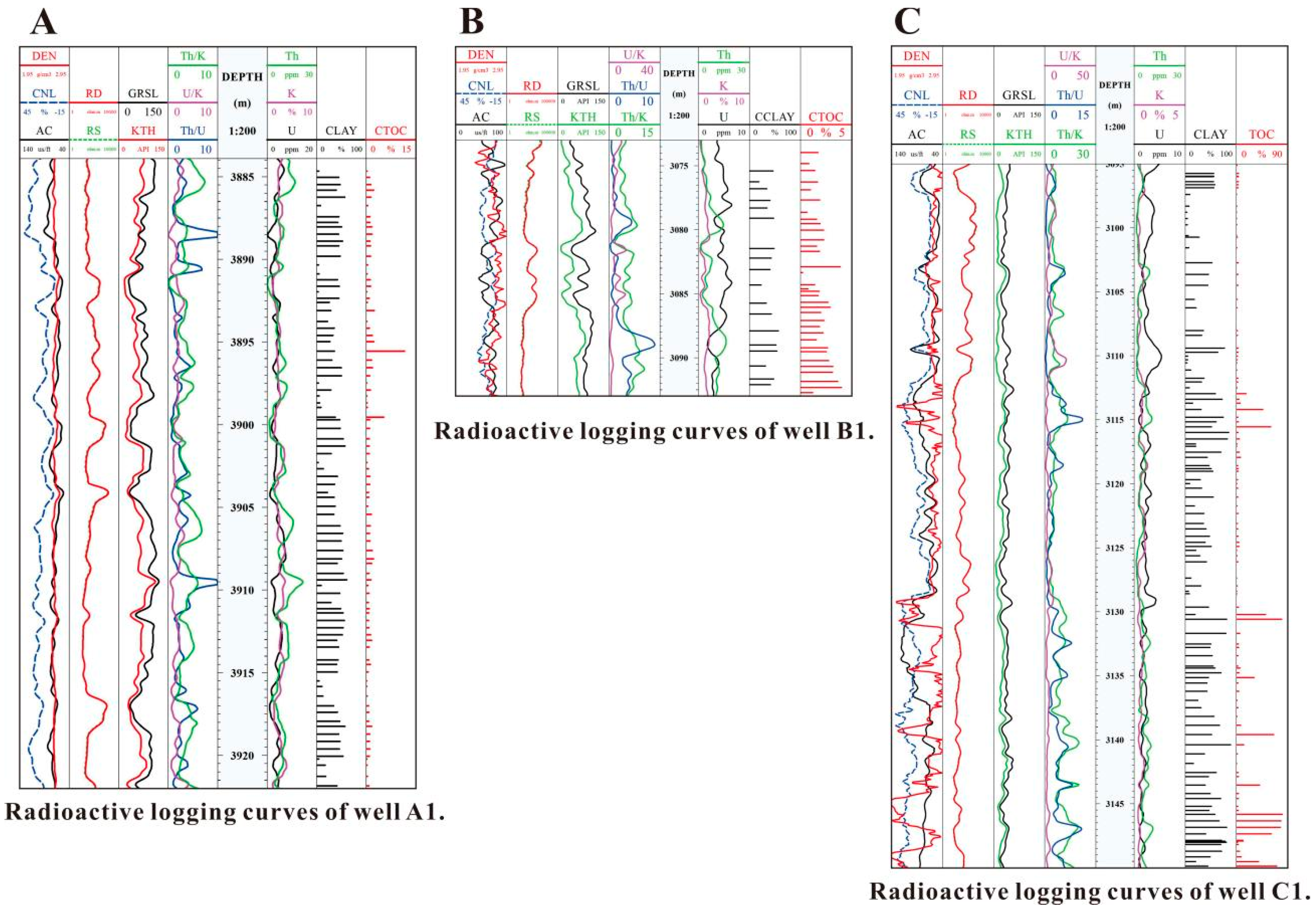
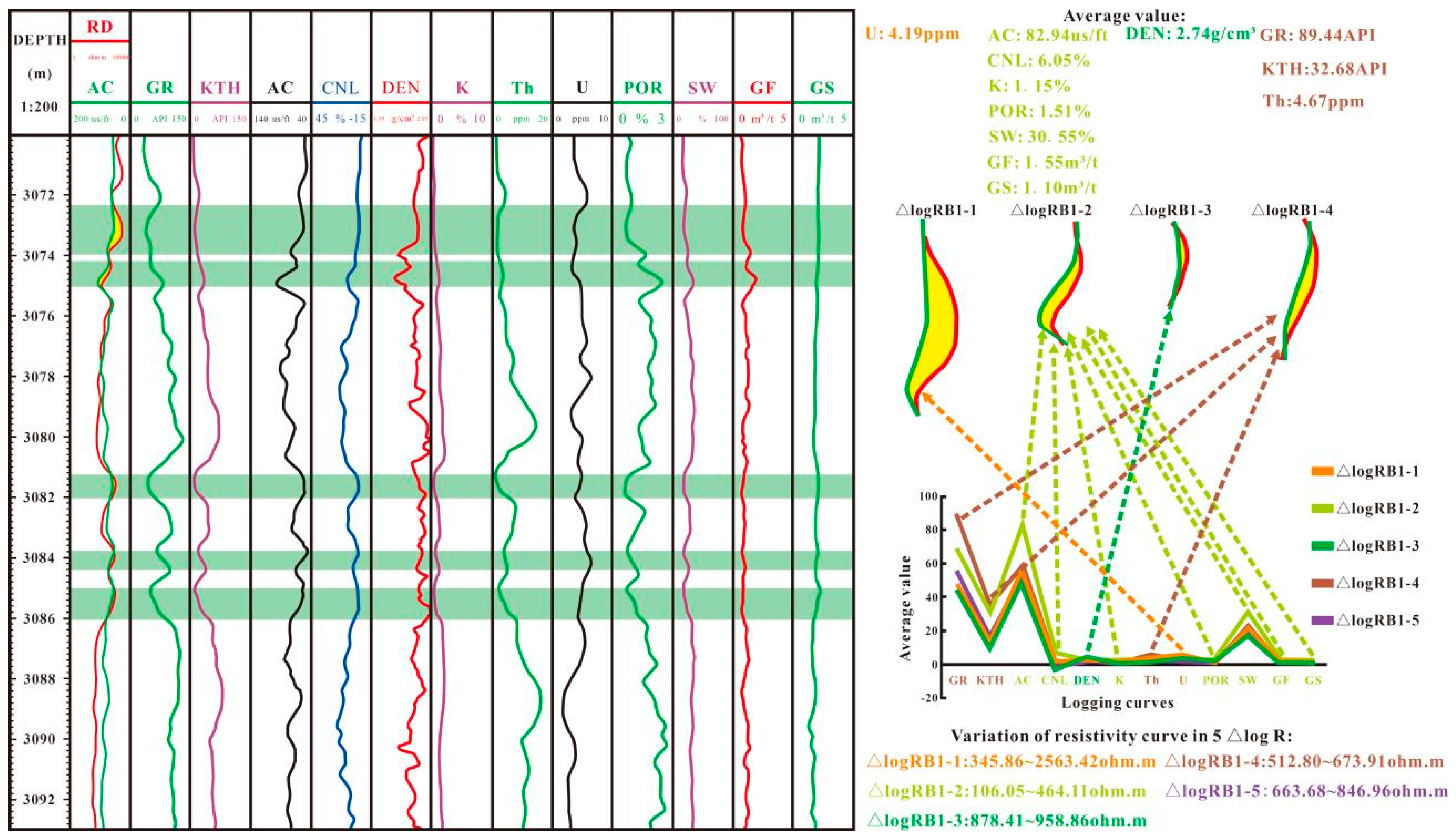
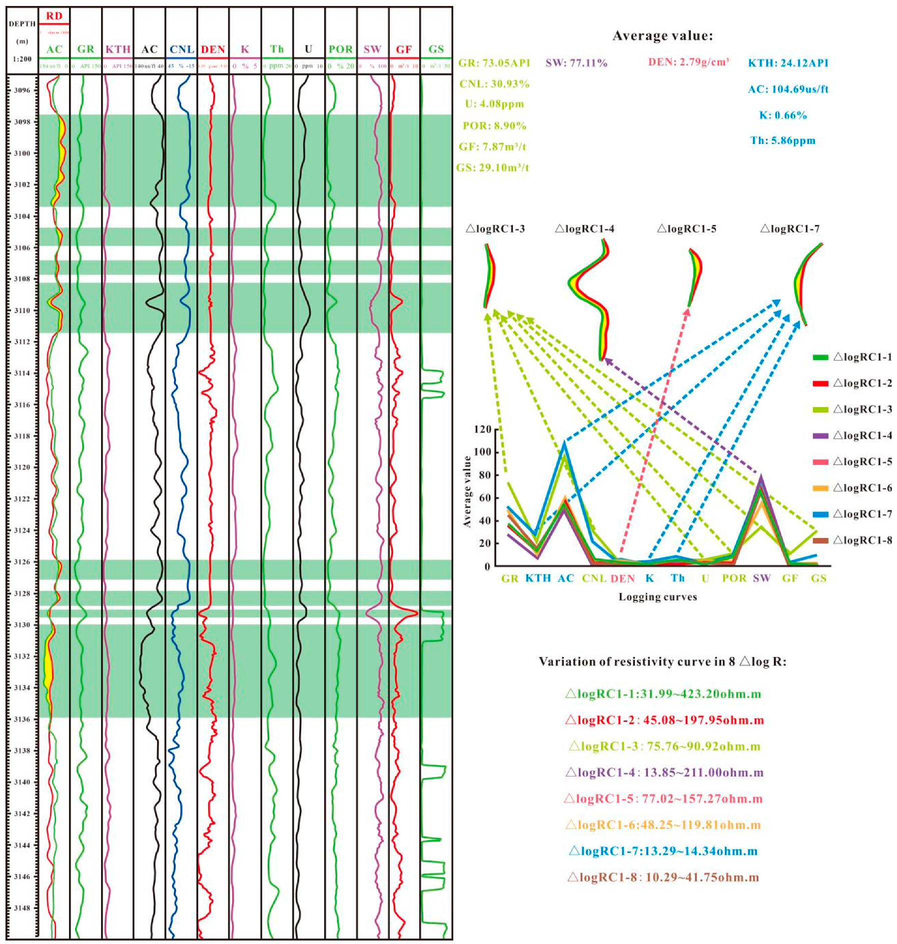
3.3. ∆log R Method Based on Natural Gamma Spectroscopy Logging Curves
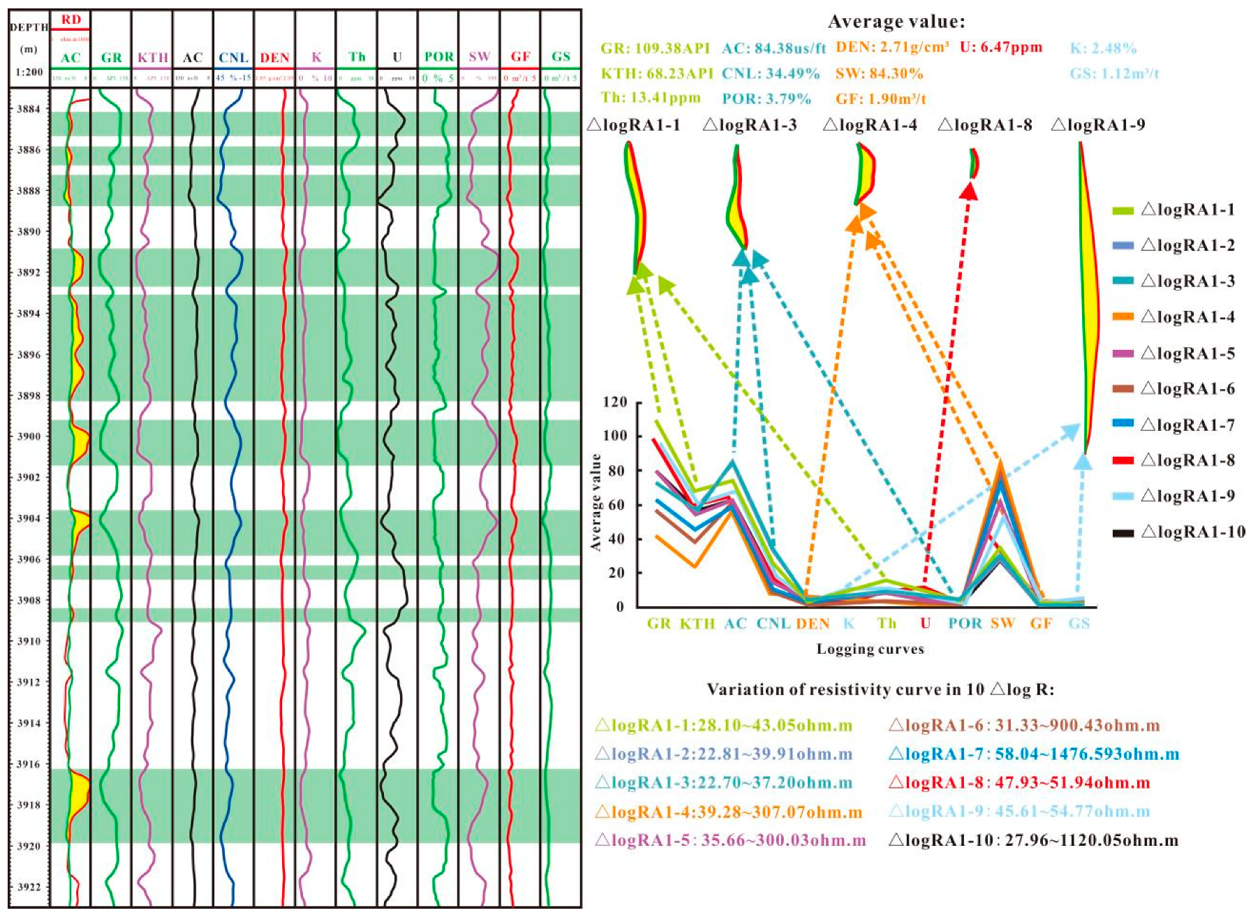
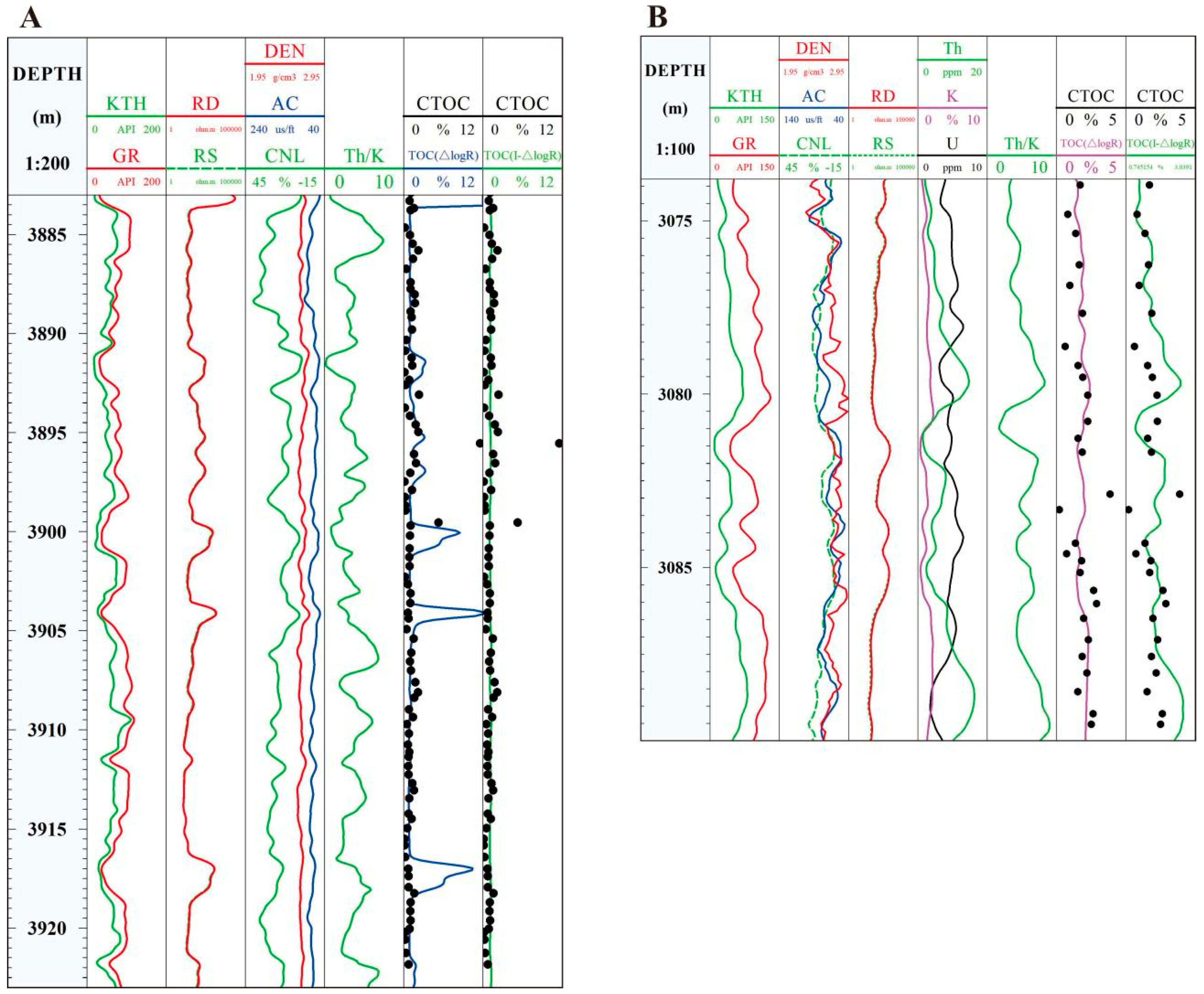
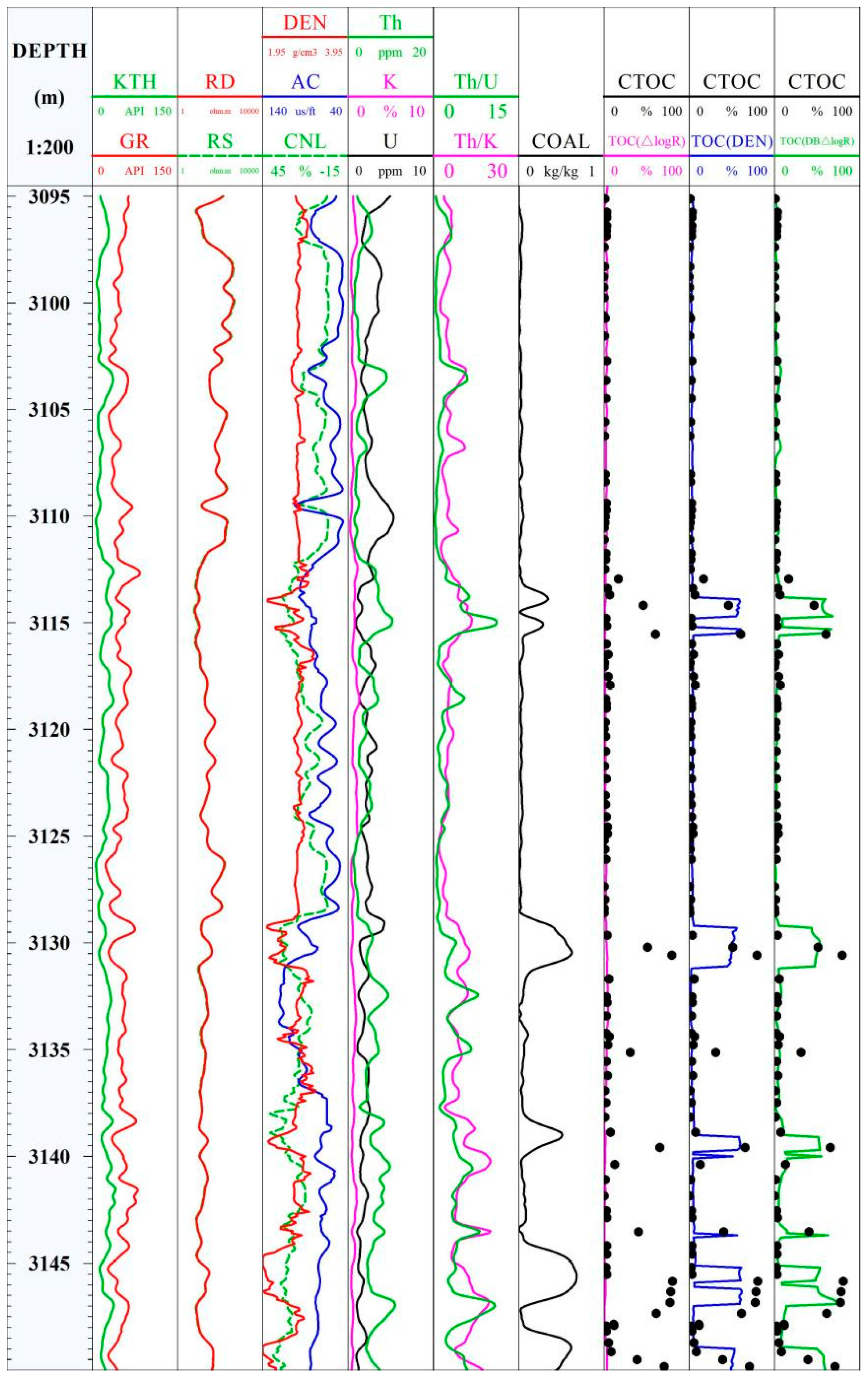
3.4. Dual ∆log R Method Based on Natural Gamma Spectroscopy Logging
4. Results
4.1. Overlapping Shapes of Sonic and Resistivity Curves and Reservoir Parameters
4.2. ∆log R Method Based on Natural Gamma Spectroscopy Logging Curves
4.3. Dual ∆log R Method Based on Natural Gamma Spectroscopy Logging
5. Discussion
6. Conclusions
Author Contributions
Funding
Acknowledgments
Conflicts of Interest
References
- Li, S.-Z.; Zhou, Z.; Nie, H.-K.; Zhang, L.-F.; Song, T.; Liu, W.-B.; Li, H.-H.; Xu, Q.-C.; Wei, S.-Y.; Tao, S. Distribution characteristics, exploration and development, geological theories research progress and exploration directions of shale gas in China. China Geol. 2022, 5, 110–135. [Google Scholar] [CrossRef]
- Zhang, J.; Shi, M.; Wang, D.; Tong, Z.; Hou, X.; Niu, J.; Li, X.; Li, Z.; Zhang, P.; Huang, Y. Fields and directions for shale gas exploration in China. Nat. Gas Explain. 2022, 9, 20–32. [Google Scholar] [CrossRef]
- Xu, S.; Hao, F.; Shu, Z.; Zhang, A.; Yang, F. Pore structures of different types of shale and shale gas exploration of the Ordovician Wufeng and Silurian Longmaxi successions in the eastern Sichuan Basin, South China. J. Asian Earth Sci. 2020, 193, 104271. [Google Scholar] [CrossRef]
- Zou, C.N.; Pan, S.Q.; Jing, Z.H. Shale oil and gas revolution and its impact. Acta Pet. Sin. 2020, 41, 1–12. [Google Scholar] [CrossRef]
- Zhao, W.Z.; Jia, A.L.; Wei, Y.S. Progress in shale gas exploration in China and Prospects for future development. China Pet. Explor. 2020, 25, 31–44. [Google Scholar] [CrossRef]
- Yasin, Q.; Baklouti, S.; Khalid, P.; Ali, S.H.; Boateng, C.D.; Du, Q. Evaluation of shale gas reservoirs in complex structural enclosures: A case study from Patala Formation in the Kohat-Potwar Plateau, Pakistan. J. Pet. Sci. Eng. 2020, 198, 108–225. [Google Scholar] [CrossRef]
- Solarin, S.; Gil-alana, L.; Lafuente, C. An investigation of long range reliance on shale oil and shale gas production in the U.S. market. Energy 2020, 195, 116933. [Google Scholar] [CrossRef]
- Ali, R.; Mahsa, N.; Ehsan, H. Shale gas potential of the lower Silurian hot shale in southern Iran and the Arabian Plate: Characterization of organic geochemistry. Petroleum 2022, 3, 1–10. [Google Scholar] [CrossRef]
- Rashid, A.; Siddiqui, N.A.; Ahmed, N.; Jamil, M.; El-Ghali, M.A.; Ali, S.H.; Zaidi, F.K.; Wahid, A. Field attributes and organic geochemical analysis of shale from early to middle Permian Dohol Formation, Peninsular Malaysia: Implications for hydrocarbon generation potential. J. King. Saud. Univ. Sci. 2022, 34, 102287. [Google Scholar] [CrossRef]
- Chukwuma, K.; Tsikos, H.; Wagner, N.; Frazenburg, M. Dual sea-level-climatic controls on the stratigraphic distribution of total organic carbon content and macerals in the Permian black shale of southwest Gondwana. J. Asian. Earth Sci. 2022, 188, 104495. [Google Scholar] [CrossRef]
- Saporetti, C.; Fonseca, D.; Oliveira, L.; Pereira, E.; Goliatt, L. Hybrid machine learning models for estimating total organic carbon from mineral constituents in core samples of shale gas fields. Mar. Petrol. Geol. 2022, 143, 105783. [Google Scholar] [CrossRef]
- Qi, Q.; Müller, T.M.; Pervukhina, M. Sonic QP/QS ratio as diagnostic tool for shale gas saturation. Geophysics 2017, 82, 3. [Google Scholar] [CrossRef]
- Fateh, B.; Mohammed, Y.A.; Jun, M.; Youcef, B.; Mohammed, S.J.; Eric, M.T.; Aala, A.M. Estimation of seismic wave attenuation from 3D seismic data: A case study of OBC data acquired in an offshore oilfield. Energies 2022, 15, 534. [Google Scholar] [CrossRef]
- Jun, M.; Mohammed, Y.A.; Fateh, B. A novel method for separating intrinsic and scattering attenuation for zero-offset vertical seismic profiling data. Geophys. J. Int. 2017, 211, 1655–1668. [Google Scholar] [CrossRef]
- Mathia, E.J.; Rexer, T.F.T.; Thomas, K.M. Influence of clay, calcareous microfossils, and organic matter on the nature and diagenetic evolution of pore systems in mudstones. J. Geophys. Res. Solid Earth 2018, 124, 149–174. [Google Scholar] [CrossRef]
- Passey, Q.R.; Creanry, S.; Kulla, J.B. A practical model for organic richness from porosity and resistivity logs. AAPG Bull. 1990, 74, 1777–1794. [Google Scholar] [CrossRef]
- Zhu, L.Q.; Zhang, C.M.; Zhang, Z.S. An improved method for evaluating the TOC content of a shale formation using the dual-difference Δlog R method. Mar. Petrol. Geol. 2019, 102, 800–816. [Google Scholar] [CrossRef]
- Yang, Z.; Zou, C.N. “Exploring petroleum inside source kitchen”: Connotation and prospects of source rock oil and gas. Petrol. Explor. Dev. 2019, 46, 173–183. [Google Scholar] [CrossRef]
- Wang, H.J.; Wu, W.; Chen, T.; Dong, X.J.; Wang, G.X. An improved neural network for TOC, S1 and S2 estimation based on conventional well logs. J. Petrol. Sci. Eng. 2019, 176, 664–678. [Google Scholar] [CrossRef]
- Zhu, L.Q.; Zhang, C.; Zhang, C.M.; Zhang, Z.S.; Zhou, X.Q.; Liu, W.N.; Zhu, B.Y. A new and reliable dual model- and data-driven TOC prediction concept: A TOC logging evaluation method using multiple overlapping methods integrated with semi-supervised deep learning. J. Petrol. Sci. Eng. 2020, 18, 1–16. [Google Scholar] [CrossRef]
- Dong, D.Z.; Qiu, Z.; Zhang, L.F.; Li, S.X.; Zhang, Q.; Li, X.T.; Zhang, S.R.; Liu, H.L.; Wang, Y.M. Progress on sedimentology of transitional facies shale and new discoveries of shale gas. Acta. Sedimentol. Sin. 2021, 39, 29–45. [Google Scholar] [CrossRef]
- Guan, Q.Q. Prediction method of total organic carbon in shale oil reservoir based on PCA-CNN model. Petro. Geol. Rec. Effic. 2022, 29, 1–9. [Google Scholar] [CrossRef]
- Liu, C.; Lu, S.; Xue, H.T. Variable-coefficient Δlog R model and its application in shale organic evaluation. Prog. Geophys. 2014, 29, 312–317. [Google Scholar] [CrossRef]
- Zhao, P.; Ma, H.; Rasouli, V. An improved model for estimating the toc in shale formations. Mar. Petrol. Geol. 2017, 83, 174–183. [Google Scholar] [CrossRef]
- Chen, H.; Liu, L.F.; Dou, W.C. Optimal selection and application of prediction methods for TOC of source rocks based on logging data in Juyanhai Depression, Yingen-Ejin Banner Basin. Prog. Geophy. 2019, 34, 1017–1024. [Google Scholar] [CrossRef]
- Luo, Y.C.; Zhang, C.M.; Zhang, Z.S.; Shi, W.R.; Liu, W.N.; Zhou, X.Q.; Zhang, Y.N. Application of continental shale gas reservoir based on improved log R method-taking X formation in D area of Sichuan Basin as an example. J. Northeast. Petro. Univ. 2021, 45, 80–90. [Google Scholar] [CrossRef]
- Li, M.L.; Zhang, C.M. An improved method for improving the calculation accuracy of marine low-resistance shale reservoir parameters. Front. Earth Sci. 2022, 10, 1–21. [Google Scholar] [CrossRef]
- Miu, H.; Wang, Y.B.; Ma, Z.T.; Guo, J.Y.; Zhang, Y.J. Generalized Δlog R model with spontaneous potential and its application in predicting total organ carbon content. J. Min. Sci. Technol. 2022, 7, 417–426. [Google Scholar] [CrossRef]
- Li, Q.W.; Liu, Z.B.; Chen, F.R.; Liu, G.Y.; Zhang, D.W.; Li, P.; Wang, P.W. Lithofacies types and reservoir characteristics of Jurassic shale in the Sichuan Basin revealed by the Da’anzhai Member, Well Y2, Yuanba area. Oil. Gas. Geol. 2022, 43, 1127–1140. [Google Scholar] [CrossRef]
- Ma, Y.S.; Cai, X.Y.; Zhao, P.R. Geological characteristics and exploration practices of continental shale oil in China. Acta. Geol. Sin. 2022, 96, 155–171. [Google Scholar] [CrossRef]
- Zhou, W.; Jiang, Z.X.; Qiu, H.Y. Shale gas accumulation conditions and prediction of favorable ares for the Lower Carboniferous Luzhai Formation in Guizhong depression. Acta. Geol. Sin. 2019, 40, 798–812. [Google Scholar] [CrossRef]
- Ou, X.Y.; Shi, K.; Mo, Y.J.; Yang, F.Q.; Li, H.L.; Zhu, G.Q. Application of comprehensive geophysical exploration in shale gas potential investigation in Guizhong depression. Prog. Geophy. 2021, 36, 1597–1606. [Google Scholar] [CrossRef]
- Tao, J.Y.; Shen, B.J.; Hu, Z.Q.; Pan, A.Y. Pore characteristics and evaluation of shale reservoir in Lower Carboniferous Luzhai Formation, northern part of middle Guangxi Depression. Petrol. Reserv. Eval. Dev. 2022, 12, 438–444. [Google Scholar] [CrossRef]
- Zhang, J.; Li, Z.; Wang, D.; Xu, L.; Li, Z.; Niu, J.; Chen, L.; Sun, Y.; Li, Q.; Yang, Z.; et al. Shale gas accumulation patterns in China. Nat. Gas. Ind. 2022, 42, 78–95. [Google Scholar] [CrossRef]
- Li, J.; Wang, X.; Zhou, K.; Wang, Y.; Li, N.; Wu, Y.; Wang, M. Characteristics of ultra-deep shale reservoir of marine-continental transitional facies: A case study of lower member of Upper Permian Longtan Formation in well Y4, Puguang Gas Field, northeastern Sichuan Basin. Petrol. Geol. Exp. 2022, 44, 71–83. [Google Scholar] [CrossRef]
- Wu, X.G.; Miu, X.X.; Wang, Z.W.; Kang, J.Y. Application of Natural Gamma Spectrometry Logging in Mineral Resources Exploration in Sichuan Basin. Spec. Oil Gas Reserv. 2021, 28, 45–52. [Google Scholar] [CrossRef]
- Luo, S.Y.; Chen, X.H.; Ni, F.J. Application of Natural Gamma Spectroscopy Logging in Evaluation and Guidance of Black Shale. Well Logging Technol. 2021, 45, 297–304. [Google Scholar] [CrossRef]
- Korun, M.; Vodenikb, B.; Zorko, B. Evaluation of gamma-ray spectrometric results near the decision threshold. Appl. Radiat. Isot. 2013, 73, 1–8. [Google Scholar] [CrossRef]
- Tan, J.J.; Wu, K.J.; Li, Y.H.; Zhao, X.Y.; Yan, C.M.; Huang, Z.H.; Du, Z.K.; Li, S. Application of logging prediction TOC method in shale reservoir evaluation. Prog. Geophys. 2021, 36, 258–266. [Google Scholar] [CrossRef]


| Core TOC | Organic Microfraction Analysis | Vitrinite Reflectance | |||||
|---|---|---|---|---|---|---|---|
| Depth (m) | TOC (w%) | Depth (m) | Vitrinite (%) | Inertinite (%) | Secondary Components (%) | Depth (m) | Ro (%) |
| 3884.67 | 0.21 | 3882.07 | 86.2 | 13.8 | 0 | 3883.68 | 1.33 |
| 3885.04 | 0.98 | 3882.89 | 88 | 12 | 0 | 3891.63 | 1.35 |
| 3885.48 | 1.35 | 3883.68 | 54.9 | 42.1 | 3 | 3900.22 | 1.28 |
| 3885.81 | 2.2 | 3885.04 | 68.5 | 22.4 | 9.1 | 3909.38 | 1.31 |
| 3886.24 | 1.4 | 3885.81 | 79.6 | 15 | 5.4 | 3917.94 | 1.38 |
| 3886.75 | 0.41 | 3887.42 | 56.6 | 11 | 32.4 | ||
| 3887.42 | 1.06 | 3888.03 | 74.3 | 13.1 | 12.6 | ||
| 3887.77 | 1.05 | 3888.90 | 80.2 | 8.5 | 11.3 | ||
| 3888.03 | 1.65 | 3891.63 | 70.1 | 20.1 | 9.8 | ||
| 3888.48 | 1.71 | 3896.10 | 82.2 | 16.8 | 1 | ||
| 3888.90 | 1.08 | 3897.05 | 74 | 25 | 1 | ||
| 3889.18 | 1.23 | 3897.90 | 73 | 22 | 5 | ||
| 3889.81 | 1.27 | 3899.55 | 84.4 | 13.6 | 2 | ||
| 3890.34 | 0.42 | 3900.22 | 88.1 | 10.4 | 1.5 | ||
| 3890.88 | 0.22 | 3901.29 | 91.5 | 8.5 | 0 | ||
| 3891.23 | 1.19 | 3904.39 | 90 | 10 | 0 | ||
| 3891.63 | 1.29 | 3906.12 | 76 | 24 | 0 | ||
| 3891.97 | 0.14 | 3907.03 | 88.9 | 11.1 | 0 | ||
| 3892.36 | 0.86 | 3907.61 | 85.7 | 14.3 | 0 | ||
| 3892.60 | 0.31 | 3908.39 | 83.6 | 16.4 | 0 | ||
| 3893.10 | 2.35 | 3909.38 | 87.5 | 9.3 | 3.2 | ||
| 3893.75 | 0.19 | 3910.76 | 84.3 | 6.8 | 8.9 | ||
| 3894.16 | 0.93 | 3911.38 | 90.4 | 3.3 | 6.3 | ||
| 3894.60 | 1.8 | 3912.71 | 79.8 | 4.8 | 15.4 | ||
| 3894.98 | 2.25 | 3913.45 | 76.7 | 15.8 | 7.5 | ||
| 3895.55 | 11.55 | 3914.50 | 40 | 12 | 48 | ||
| 3896.10 | 1.56 | 3917.01 | 82.3 | 4.3 | 13.4 | ||
| 3896.56 | 1.87 | 3917.94 | 81 | 4 | 15 | ||
| 3897.05 | 1.01 | 3918.71 | 92 | 7 | 1 | ||
| 3897.48 | 0.13 | 3920.05 | 82 | 15 | 3 | ||
| 3897.90 | 1.24 | ||||||
| 3898.26 | 0.18 | ||||||
| 3898.68 | 0.26 | ||||||
| 3898.95 | 0.31 | ||||||
| Core TOC | Organic Microfraction Analysis | Vitrinite Reflectance | |||||
|---|---|---|---|---|---|---|---|
| Depth (m) | TOC (w%) | Depth (m) | Exinite (%) | Vitrinite (%) | Inertinite (%) | Depth (m) | Ro (%) |
| 3069.80 | 0.81 | 3077.67 | 43 | 50 | 7 | 3077.67 | 3.69 |
| 3070.97 | 1.71 | 3080.79 | 57 | 37 | 6 | 3080.79 | 3.67 |
| 3072.77 | 2.16 | 3085.15 | 52 | 45 | 3 | 3085.15 | 3.79 |
| 3072.95 | 0.5 | 3086.47 | 58 | 38 | 4 | 3086.47 | 3.86 |
| 3073.97 | 1.7 | 3089.22 | 54 | 40 | 6 | 3089.22 | 4.02 |
| 3074.82 | 0.81 | 3090.68 | 45 | 52 | 3 | 3090.68 | 3.64 |
| 3075.37 | 1.4 | 3091.85 | 42 | 52 | 6 | 3091.85 | 4.12 |
| 3076.27 | 1.65 | 3092.73 | 45 | 47 | 8 | 3092.73 | 3.88 |
| 3076.87 | 0.96 | 3093.67 | 68 | 28 | 4 | 3093.67 | 3.65 |
| 3077.67 | 1.87 | 3102.26 | 70 | 24 | 6 | 3102.26 | 3.64 |
| 3078.63 | 0.63 | 3107.31 | 48 | 46 | 6 | 3107.31 | 3.81 |
| 3079.18 | 1.57 | ||||||
| 3079.52 | 1.91 | ||||||
| 3080.03 | 2.25 | ||||||
| 3080.79 | 2.27 | ||||||
| 3081.28 | 1.57 | ||||||
| 3081.68 | 1.85 | ||||||
| 3082.89 | 3.88 | ||||||
| 3083.34 | 0.2 | ||||||
| 3084.30 | 1.38 | ||||||
| 3084.61 | 0.74 | ||||||
| 3084.81 | 1.81 | ||||||
| 3085.15 | 1.72 | ||||||
| 3085.67 | 2.68 | ||||||
| 3086.05 | 2.9 | ||||||
| 3086.47 | 1.97 | ||||||
| 3087.09 | 2.3 | ||||||
| 3087.57 | 1.85 | ||||||
| 3088.05 | 2.2 | ||||||
| 3088.59 | 1.53 | ||||||
| 3089.22 | 2.64 | ||||||
| 3089.53 | 2.51 | ||||||
| 3090.23 | 2.75 | ||||||
| 3090.68 | 3.15 | ||||||
| 3091.13 | 3.13 | ||||||
| 3091.85 | 3.64 | ||||||
| 3092.33 | 4 | ||||||
| 3092.73 | 1.19 | ||||||
| 3093.21 | 0.44 | ||||||
| 3093.67 | 0.53 | ||||||
| 3095.27 | 2.25 | ||||||
| 3095.45 | 1.23 | ||||||
| 3098.38 | 0.18 | ||||||
| 3101.39 | 0.65 | ||||||
| 3107.31 | 1.49 | ||||||
| 3110.43 | 0.34 | ||||||
| Core TOC | Organic Microfraction Analysis | Vitrinite Reflectance | ||||||
|---|---|---|---|---|---|---|---|---|
| Sample | TOC (w%) | Sample | Sapropelinite (%) | Vitrinite (%) | Inertinite (%) | Secondary Components (%) | Sample | Ro (%) |
| 3100.61 | 0.13 | 3095.98 | 0 | 75 | 25 | 0 | 3095.98 | 1.86 |
| 3100.74 | 1.61 | 3100.74 | 0 | 69.7 | 30.3 | 0 | 3109.72 | 1.93 |
| 3101.56 | 0.74 | 3102.73 | 0 | 76.6 | 18.4 | 5 | 3116.00 | 1.96 |
| 3102.73 | 3.23 | 3109.72 | 0 | 73.6 | 26.4 | 0 | 3124.58 | 2.01 |
| 3103.64 | 2.52 | 3112.96 | 0 | 62 | 34 | 4 | 3130.21 | 2.08 |
| 3104.49 | 2.6 | 3114.20 | 0 | 77.3 | 22.7 | 0 | 3144.21 | 2.07 |
| 3105.59 | 1.45 | 3116.00 | 0 | 71.9 | 24.6 | 3.5 | 3150.41 | 2.67 |
| 3106.26 | 0.91 | 3117.53 | 0 | 67.5 | 22.1 | 5.4 | 3164.33 | 2.13 |
| 3108.04 | 1.69 | 3118.82 | 0 | 68.3 | 31.7 | 0 | 3172.65 | 2.16 |
| 3108.4 | 1.81 | 3121.04 | 3 | 64 | 20 | 13 | 3178.06 | 2.32 |
| 3109.4 | 2.88 | 3124.58 | 0 | 70.6 | 19.4 | 10 | ||
| 3109.72 | 2.85 | 3126.10 | 0 | 90 | 10 | 0 | ||
| 3110.03 | 1.9 | 3130.21 | 0 | 65 | 35 | 0 | ||
| 3110.31 | 1.42 | 3134.40 | 0 | 66 | 34 | 0 | ||
| 3110.55 | 0.56 | 3138.88 | 0 | 67.3 | 21.4 | 11.3 | ||
| 3111.12 | 0.6 | 3140.40 | 0 | 63.8 | 26.2 | 0 | ||
| 3111.75 | 2.68 | 3144.21 | 2 | 54.6 | 37.4 | 6 | ||
| 3112.05 | 2.12 | 3147.86 | 0 | 62 | 38 | 0 | ||
| 3112.5 | 1.13 | 3148.72 | 0 | 69.7 | 30.3 | 0 | ||
| 3112.96 | 16.86 | 3150.41 | 0 | 80 | 20 | 0 | ||
| 3113.4 | 4.31 | 3152.6 | 0 | 53.9 | 46.1 | 14.4 | ||
| 3113.7 | 6.71 | 3156.21 | 0 | 83.1 | 16.9 | 0 | ||
| 3114.2 | 46.3 | 3163.95 | 0 | 69.7 | 30.3 | 0 | ||
| 3114.8 | 2.48 | 3167.79 | 0 | 65 | 35 | 0 | ||
| 3115.16 | 3.39 | 3170.615 | 0 | 74 | 20 | 6 | ||
| 3115.55 | 60.46 | 3174.26 | 0 | 71.8 | 28.2 | 0 | ||
| 3116 | 2.89 | 3176.71 | 0 | 59 | 41 | 0 | ||
| 3116.5 | 5.1 | 3178.06 | 0 | 69 | 31 | 0 | ||
| 3116.89 | 1.09 | 3179.52 | 0 | 75 | 25 | 0 | ||
| 3117.07 | 0.49 | |||||||
| 3117.53 | 5.01 | |||||||
| 3117.94 | 7.19 | |||||||
| 3118.58 | 2.21 | |||||||
| 3118.82 | 3.08 | |||||||
| 3119.02 | 3.09 | |||||||
| 3119.69 | 1.93 | |||||||
| 3119.99 | 0.63 | |||||||
| 3120.35 | 2.06 | |||||||
| 3121.04 | 2.36 | |||||||
| 3121.73 | 1.04 | |||||||
| 3122.32 | 2.81 | |||||||
| 3123.1 | 1.74 | |||||||
| 3123.53 | 2.34 | |||||||
| 3124.11 | 2.88 | |||||||
| 3124.58 | 4.09 | |||||||
| 3124.9 | 4.41 | |||||||
| 3125.2 | 0.47 | |||||||
| 3125.63 | 1.15 | |||||||
| 3126.1 | 2.42 | |||||||
| 3127.37 | 0.37 | |||||||
| 3127.98 | 1.5 | |||||||
| 3128.4 | 0.48 | |||||||
| 3128.6 | 0.61 | |||||||
| 3129.65 | 3.66 | |||||||
| 3130.21 | 51.27 | |||||||
| 3130.59 | 79.58 | |||||||
| 3131.7 | 5.82 | |||||||
| 3132.53 | 3.21 | |||||||
| 3132.8 | 3.83 | |||||||
| 3133.43 | 2.82 | |||||||
| 3134.25 | 2.5 | |||||||
| 3134.4 | 6.36 | |||||||
| 3134.78 | 4.57 | |||||||
| 3135.14 | 31.14 | |||||||
| 3135.57 | 2.84 | |||||||
| 3136.22 | 4.15 | |||||||
| 3136.93 | 1.35 | |||||||
| 3137.5 | 2.65 | |||||||
| 3138.18 | 1.13 | |||||||
| 3138.88 | 7.53 | |||||||
| 3139.6 | 65.63 | |||||||
| 3140.4 | 12.88 | |||||||
| 3141.1 | 1.62 | |||||||
| 3141.86 | 0.45 | |||||||
| 3142.56 | 2.96 | |||||||
| 3142.88 | 3.55 | |||||||
| Well | DEPTH (m) | GRSL (API) | U (ppm) | CCLAY (%) | CTOC (%) | Th/U | U/K | Th/K |
|---|---|---|---|---|---|---|---|---|
| A1 | 3883.9–3894.7 | 73.98 | 3.5 | 33.7 | 1.05 | 3.55 | 1.68 | 3.33 |
| 3894.7–3922.0 | 81.56 | 3.85 | 36.16 | 1.14 | 2.56 | 1.63 | 3.6 | |
| B1 | 3073.0–3075.6 | 51.33 | 4.07 | 46.2 | 1.3 | 0.68 | 6.03 | 3.74 |
| 3075.6–3093.0 | 80.49 | 4.32 | 40.33 | 2.09 | 2.48 | 3.87 | 6.01 | |
| C1 | 3100.0–3125.2 | 36.71 | 2.53 | 37.71 | 4.90 | 2.01 | 4.76 | 5.81 |
| 3125.3–3150.0 | 35.25 | 1.86 | 49.83 | 17.31 | 3.54 | 3.37 | 9.78 |
| Coefficients | |
|---|---|
| Intercept | 0.1394 |
| X Variable 1 () | 0.2903 |
| X Variable 2 () | 0.3734 |
| Coefficients | |
|---|---|
| Intercept | 1.7000 |
| X Variable 1 () | 0.1192 |
| X Variable 2 () | 0.1316 |
| Coefficients | |
|---|---|
| Intercept | 39.3652 |
| X Variable 1 () | 3.3658 |
| X Variable 2 () | −0.0921 |
| Coefficients | |
|---|---|
| Intercept | −2.2084 |
| X Variable 1 () | 0.8459 |
| X Variable 2 () | −0.2995 |
| ∆log RA1-1 | ∆log RA1-3 | ∆log RA1-4 | |||||||||
|---|---|---|---|---|---|---|---|---|---|---|---|
| DEPTH (m) | GR (API) | KTH (API) | TH (ppm) | DEPTH (m) | AC (us/ft) | CNL (%) | POR (%) | DEPTH (m) | DEN (g/cm3) | SW (%) | GF (m3/t) |
| 3884.24 | 110.21 | 73.77 | 13.30 | 3887.25 | 83.17 | 32.54 | 3.79 | 3891.05 | 2.75 | 90.06 | 1.98 |
| 3884.34 | 110.58 | 70.69 | 13.10 | 3887.35 | 83.78 | 33.24 | 3.82 | 3891.15 | 2.75 | 95.04 | 2.13 |
| 3884.44 | 110.20 | 67.37 | 12.93 | 3887.45 | 83.66 | 33.61 | 3.83 | 3891.25 | 2.74 | 97.33 | 2.22 |
| 3884.54 | 109.61 | 65.18 | 12.89 | 3887.55 | 82.84 | 33.48 | 3.81 | 3891.35 | 2.73 | 97.58 | 2.24 |
| 3884.64 | 109.11 | 64.83 | 13.05 | 3887.65 | 81.96 | 33.00 | 3.66 | 3891.45 | 2.72 | 96.80 | 2.22 |
| 3884.74 | 108.74 | 66.09 | 13.43 | 3887.75 | 81.56 | 32.47 | 3.57 | 3891.55 | 2.71 | 95.87 | 2.19 |
| 3884.84 | 108.45 | 67.92 | 13.95 | 3887.85 | 81.90 | 32.26 | 3.65 | 3891.65 | 2.70 | 95.13 | 2.17 |
| 3884.95 | 108.14 | 69.97 | 14.61 | 3887.95 | 83.10 | 32.71 | 3.80 | 3891.75 | 2.70 | 94.35 | 2.14 |
| 3888.05 | 85.51 | 33.94 | 3.88 | 3891.85 | 2.69 | 93.09 | 2.11 | ||||
| 3888.15 | 88.64 | 35.85 | 3.99 | 3891.95 | 2.69 | 91.00 | 2.04 | ||||
| 3888.25 | 90.60 | 37.81 | 4.08 | 3892.05 | 2.69 | 87.73 | 1.95 | ||||
| 3888.35 | 90.13 | 38.89 | 4.03 | 3892.15 | 2.70 | 83.29 | 1.83 | ||||
| 3888.45 | 87.23 | 38.47 | 3.93 | 3892.25 | 2.70 | 77.57 | 1.67 | ||||
| 3888.55 | 83.18 | 36.20 | 3.69 | 3892.35 | 2.70 | 70.66 | 1.49 | ||||
| 3888.65 | 78.46 | 32.83 | 3.36 | 3892.45 | 2.70 | 62.99 | 1.38 | ||||
| 3892.55 | 2.69 | 55.46 | 1.20 | ||||||||
| 3892.65 | 2.68 | 49.21 | 1.28 | ||||||||
| ∆log RA1-8 | ∆log RA1-9 | |||
|---|---|---|---|---|
| DEPTH (m) | U (ppm) | DEPTH (m) | K (%) | GS (m3/t) |
| 3906.37 | 6.03 | 3908.47 | 2.53 | 1.20 |
| 3906.47 | 6.30 | 3908.57 | 2.49 | 1.15 |
| 3906.57 | 6.47 | 3908.67 | 2.47 | 1.11 |
| 3906.67 | 6.60 | 3908.77 | 2.46 | 1.08 |
| 3906.77 | 6.69 | 3908.87 | 2.48 | 1.07 |
| 3906.87 | 6.72 | |||
| ∆log RA1-1 | ∆log RA1-2 | ∆log RA1-3 | ∆log RA1-4 | ||||||||||||
|---|---|---|---|---|---|---|---|---|---|---|---|---|---|---|---|
| DEPTH (m) | U (ppm) | DEPTH (m) | AC (us/ft) | CNL (%) | K (%) | POR (%) | SW (%) | GF (m3/t) | GS (m3/t) | DEPTH (m) | DEN (g/cm3) | DEPTH (m) | GR (API) | KTH (API) | Th (ppm) |
| 3072.50 | 4.63 | 3074.38 | 63.11 | 0.82 | 0.94 | 1.23 | 23.98 | 1.08 | 0.64 | 3081.50 | 2.74 | 3084.13 | 85.43 | 30.24 | 4.49 |
| 3072.63 | 4.60 | 3074.50 | 69.91 | 3.26 | 1.04 | 1.32 | 26.46 | 1.24 | 0.84 | 3081.63 | 2.75 | 3084.25 | 93.44 | 35.12 | 4.85 |
| 3072.75 | 4.55 | 3074.63 | 80.89 | 7.05 | 1.16 | 1.47 | 30.10 | 1.57 | 1.15 | ||||||
| 3072.88 | 4.40 | 3074.75 | 90.95 | 8.86 | 1.25 | 1.61 | 33.29 | 1.89 | 1.33 | ||||||
| 3073.00 | 4.11 | 3074.88 | 96.56 | 8.46 | 1.28 | 1.70 | 34.96 | 1.89 | 1.33 | ||||||
| 3073.13 | 3.84 | 3075.00 | 96.21 | 7.85 | 1.22 | 1.70 | 34.48 | 1.62 | 1.29 | ||||||
| 3073.25 | 3.76 | ||||||||||||||
| 3073.38 | 3.84 | ||||||||||||||
| 3073.50 | 4.04 | ||||||||||||||
| 3073.63 | 4.21 | ||||||||||||||
| 3073.75 | 4.23 | ||||||||||||||
| 3073.88 | 4.13 | ||||||||||||||
| ∆log RA1-3 | ∆log RA1-4 | ∆log RA1-5 | ∆log RA1-7 | ||||||||||||
|---|---|---|---|---|---|---|---|---|---|---|---|---|---|---|---|
| DEPTH (m) | GR (API) | CNL (%) | U (ppm) | POR (%) | GF (m3/t) | GS (m3/t) | DEPTH (m) | SW (%) | DEPTH (m) | DEN (g/cm3) | DEPTH (m) | KTH (API) | AC (us/ft) | K (%) | Th (ppm) |
| 3129.10 | 69.83 | 26.55 | 4.26 | 8.25 | 7.24 | 2.91 | 3125.90 | 74.47 | 3104.50 | 2.71 | 3129.80 | 21.53 | 86.10 | 0.54 | 5.73 |
| 3129.20 | 72.81 | 30.96 | 4.20 | 9.03 | 8.95 | 35.59 | 3126.00 | 75.70 | 3104.60 | 2.72 | 3129.90 | 19.52 | 84.87 | 0.52 | 5.64 |
| 3129.30 | 74.94 | 32.13 | 4.13 | 9.18 | 9.12 | 36.26 | 3126.10 | 77.09 | 3104.70 | 2.75 | 3130.00 | 17.63 | 83.64 | 0.50 | 5.49 |
| 3129.40 | 75.28 | 33.10 | 4.06 | 9.16 | 8.27 | 36.45 | 3126.20 | 78.37 | 3104.80 | 2.78 | 3130.10 | 15.93 | 82.23 | 0.46 | 5.25 |
| 3129.50 | 72.36 | 31.91 | 3.75 | 8.86 | 5.79 | 34.29 | 3126.30 | 79.26 | 3104.90 | 2.77 | 3130.20 | 14.35 | 75.83 | 0.41 | 4.96 |
| 3126.40 | 79.58 | 3105.00 | 2.77 | 3130.30 | 13.08 | 76.08 | 0.38 | 4.71 | |||||||
| 3126.50 | 79.32 | 3105.10 | 2.77 | 3130.40 | 12.44 | 78.15 | 0.36 | 4.58 | |||||||
| 3126.60 | 78.70 | 3105.20 | 2.78 | 3130.50 | 12.37 | 81.81 | 0.35 | 4.50 | |||||||
| 3126.70 | 77.73 | 3105.30 | 2.79 | 3130.60 | 12.54 | 91.80 | 0.35 | 4.39 | |||||||
| 3126.80 | 76.40 | 3105.40 | 2.79 | 3130.70 | 12.98 | 97.40 | 0.35 | 4.29 | |||||||
| 3126.90 | 74.96 | 3105.50 | 2.80 | 3130.80 | 13.87 | 103.13 | 0.36 | 4.27 | |||||||
| 3127.00 | 73.71 | 3105.60 | 2.81 | 3130.90 | 15.29 | 107.07 | 0.39 | 4.37 | |||||||
| 3105.70 | 2.82 | 3131.00 | 17.09 | 110.80 | 0.44 | 4.50 | |||||||||
| 3105.80 | 2.82 | 3131.10 | 18.90 | 112.91 | 0.50 | 4.63 | |||||||||
| 3105.90 | 2.82 | 3131.20 | 20.51 | 114.77 | 0.54 | 4.74 | |||||||||
| 3106.00 | 2.82 | 3131.30 | 21.91 | 115.20 | 0.57 | 4.86 | |||||||||
| 3106.10 | 2.82 | 3131.40 | 23.14 | 115.34 | 0.59 | 5.02 | |||||||||
| 3106.20 | 2.80 | 3131.50 | 24.17 | 115.44 | 0.60 | 5.21 | |||||||||
| 3131.60 | 24.93 | 115.33 | 0.61 | 5.49 | |||||||||||
| 3131.70 | 25.60 | 115.19 | 0.62 | 5.96 | |||||||||||
| 3131.80 | 26.38 | 115.59 | 0.64 | 6.60 | |||||||||||
| 3131.90 | 27.35 | 115.12 | 0.66 | 7.24 | |||||||||||
| 3132.00 | 28.51 | 118.83 | 0.69 | 7.79 | |||||||||||
| 3132.10 | 29.67 | 119.13 | 0.72 | 8.26 | |||||||||||
| 3132.20 | 30.59 | 119.26 | 0.74 | 8.72 | |||||||||||
| 3132.30 | 31.16 | 119.13 | 0.76 | 9.13 | |||||||||||
| 3132.40 | 31.65 | 118.96 | 0.77 | 9.37 | |||||||||||
| 3132.50 | 32.34 | 119.10 | 0.79 | 9.38 | |||||||||||
| 3132.60 | 32.98 | 119.64 | 0.79 | 9.13 | |||||||||||
| 3132.70 | 33.17 | 120.29 | 0.80 | 8.69 | |||||||||||
| 3132.80 | 32.83 | 120.58 | 0.80 | 8.19 | |||||||||||
| 3132.90 | 32.08 | 120.22 | 0.82 | 7.67 | |||||||||||
| 3133.00 | 30.93 | 119.08 | 0.83 | 7.05 | |||||||||||
| 3133.10 | 29.76 | 117.53 | 0.85 | 6.42 | |||||||||||
| 3133.20 | 28.76 | 116.12 | 0.88 | 5.84 | |||||||||||
| 3133.30 | 27.88 | 115.65 | 0.90 | 5.36 | |||||||||||
| 3133.40 | 27.08 | 116.54 | 0.92 | 4.98 | |||||||||||
| 3133.50 | 26.52 | 118.40 | 0.94 | 4.73 | |||||||||||
| 3133.60 | 26.59 | 120.33 | 0.94 | 4.74 | |||||||||||
| 3133.70 | 27.38 | 121.11 | 0.92 | 5.02 | |||||||||||
| 3133.80 | 28.41 | 120.05 | 0.88 | 5.42 | |||||||||||
| 3133.90 | 29.14 | 116.99 | 0.84 | 5.77 | |||||||||||
| 3134.00 | 29.31 | 109.18 | 0.80 | 6.01 | |||||||||||
| 3134.10 | 29.10 | 105.97 | 0.78 | 6.21 | |||||||||||
| 3134.20 | 28.66 | 104.04 | 0.75 | 6.39 | |||||||||||
| 3134.30 | 28.03 | 104.34 | 0.74 | 6.46 | |||||||||||
| 3134.40 | 27.22 | 109.92 | 0.74 | 6.47 | |||||||||||
| 3134.50 | 26.41 | 108.61 | 0.75 | 6.49 | |||||||||||
| 3134.60 | 25.89 | 108.94 | 0.76 | 6.62 | |||||||||||
| 3134.70 | 25.77 | 108.18 | 0.77 | 6.80 | |||||||||||
| 3134.80 | 25.85 | 104.88 | 0.77 | 6.96 | |||||||||||
| 3134.90 | 25.95 | 100.95 | 0.77 | 7.07 | |||||||||||
| 3135.00 | 26.07 | 96.65 | 0.76 | 7.17 | |||||||||||
| 3135.10 | 26.18 | 94.51 | 0.74 | 7.18 | |||||||||||
| 3135.20 | 25.99 | 97.52 | 0.70 | 6.95 | |||||||||||
| 3135.30 | 25.27 | 98.07 | 0.65 | 6.43 | |||||||||||
| 3135.40 | 24.21 | 95.07 | 0.59 | 5.81 | |||||||||||
| 3135.50 | 23.25 | 94.86 | 0.56 | 5.32 | |||||||||||
| 3135.60 | 22.50 | 93.72 | 0.56 | 5.00 | |||||||||||
| 3135.70 | 21.66 | 91.81 | 0.56 | 4.73 | |||||||||||
| 3135.80 | 20.76 | 89.82 | 0.57 | 4.47 | |||||||||||
| 3135.90 | 20.15 | 88.50 | 0.58 | 4.27 | |||||||||||
| 3136.00 | 20.07 | 88.26 | 0.59 | 4.14 | |||||||||||
| 3136.10 | 20.66 | 90.16 | 0.60 | 4.10 | |||||||||||
| 3136.20 | 21.75 | 91.47 | 0.61 | 4.14 | |||||||||||
| 3136.30 | 22.72 | 94.98 | 0.62 | 4.20 | |||||||||||
| 3136.40 | 23.01 | 97.29 | 0.62 | 4.23 | |||||||||||
| 3136.50 | 22.35 | 98.32 | 0.61 | 4.20 | |||||||||||
| 3136.60 | 21.07 | 97.25 | 0.58 | 4.20 | |||||||||||
| 3136.70 | 19.70 | 94.25 | 0.54 | 4.26 | |||||||||||
Disclaimer/Publisher’s Note: The statements, opinions and data contained in all publications are solely those of the individual author(s) and contributor(s) and not of MDPI and/or the editor(s). MDPI and/or the editor(s) disclaim responsibility for any injury to people or property resulting from any ideas, methods, instructions or products referred to in the content. |
© 2023 by the authors. Licensee MDPI, Basel, Switzerland. This article is an open access article distributed under the terms and conditions of the Creative Commons Attribution (CC BY) license (https://creativecommons.org/licenses/by/4.0/).
Share and Cite
Li, M.; Zhang, C. An Improved Method to Accurately Estimate TOC of Shale Reservoirs and Coal-Measures. Energies 2023, 16, 2905. https://doi.org/10.3390/en16062905
Li M, Zhang C. An Improved Method to Accurately Estimate TOC of Shale Reservoirs and Coal-Measures. Energies. 2023; 16(6):2905. https://doi.org/10.3390/en16062905
Chicago/Turabian StyleLi, Menglei, and Chaomo Zhang. 2023. "An Improved Method to Accurately Estimate TOC of Shale Reservoirs and Coal-Measures" Energies 16, no. 6: 2905. https://doi.org/10.3390/en16062905
APA StyleLi, M., & Zhang, C. (2023). An Improved Method to Accurately Estimate TOC of Shale Reservoirs and Coal-Measures. Energies, 16(6), 2905. https://doi.org/10.3390/en16062905