Excess Anisotropy: A Method to Predict Frequency of Resistive Fractures in the Wolfcamp Shale

Abstract

A horizontal well in the Wolfcamp Formation within the Delaware Basin exhibits cross-dipole sonic log anisotropy varying from 0.0% to 29.7% over the reservoir interval. Massive limestones exhibit little anisotropy while shales and intervals with high fracture counts have high anisotropy. Integrated analysis of acoustic, image and triple combo open-hole log data indicates that the computed volume of shale log is a strong predictor of anisotropy with a simple linear relationship. However, there is much anisotropy that is not accounted for by this lithologically related linear relationship. We refer to the residual obtained by subtracting the predicted anisotropy using this relationship from the measured anisotropy from a cross-dipole sonic tool as the excess anisotropy. The excess anisotropy is the remaining anisotropy that is not accounted for by linear regression between the volume of shale log and the measured anisotropy. We find that the excess anisotropy is linearly correlated to the resistive fracture density. Linear regression between the two variables yields a statistically significant relationship that enables a rough estimation of the resistive fracture frequency from the excess anisotropy. Validation in a second well produces a similar correlation to fracture frequency.

1. Introduction

The Wolfcamp Formation is a highly variable mixed carbonate–siliciclastic and hydrocarbon-rich shale play across the Permian Basin with recovered resources of 20 million barrels of oil and 47 billion cubic feet of gas since November 2018 [1,2]. With such highly variable facies, the formation poses numerous petrophysical challenges: carbonate compositions and clastic contributions can vary greatly, and TOC varies from less than 1% to more than 6% weight percent [1,3]. The study wells are located on the north-eastern edge of the Delaware Basin off the western edge of the Central Basin Platform with carbonate composition ranging from less than 0.5% to more than 99% with TOC from 0% to 2.7% weight percent. Fracture characterization within the formation indicates a majority of calcite-healed resistive fractures in two orthogonal sets with a NE–SW orientation, which is parallel to present-day SHmax, and NW–SE trends [4]. These healed fractures can potentially inhibit fluid flow.

In the study well, a total of 1724 fractures are identified on the image log over a depth interval of 4961 feet; of these, 1547 are classified as resistive. The highly variable mixed carbonate–siliciclastic lithology, variations in TOC and two nearly orthogonal resistive fracture sets result in a highly variable measured anisotropy throughout the formation (from 0.0% to 29.7%). An accurate estimation of the fracture frequency of a formation is key for a better understanding of fluid flow and the resulting anisotropy can influence seismic wave propagation. Aligned fractures in a layered media complicate the symmetry of the anisotropy. Conversely, anisotropy alone cannot uniquely determine the fracture density. The frequency and nature of fractures can be interpreted and counted from formation image logs given sufficient data quality, thereby at least roughly quantifying the fracture density. Shear-wave anisotropy can be measured with sonic logs. We wish to determine if measured anisotropy can be used to indicate the frequency of fractures seen on image logs. The purpose of this paper is specifically to estimate fracture frequency from measured anisotropy. To do this, other factors contributing to anisotropy must first be removed. If successful, such a characterization could be potentially useful in estimating relative fracture density in the absence of image logs or, similarly, enabling the interpretation of fracture density from surface or borehole seismic anisotropy measurements.

Interpretative methods currently used to identify fractures involve workflows that are both expensive and time-consuming due to the time and knowledge necessary to process, evaluate and interpret all the quad combo and image data [2,5], leading to increased operational costs and delayed decision-making. Alternatively, fracture frequency prediction from conventional well logs without the use of image data would be of practical benefit as oil and gas operators and service companies have interest in automating workflows and utilizing predictive techniques to aid in improving the interpretation of available data to rapidly supplement more time-consuming interpretation techniques. Guo et al. [6] predicted the intensity and direction of high-angle fractures in the Devonian shale in the Western Canada Basin from azimuthal, prestack seismic-anisotropy inversion, while Pollock et al. [7] predicted fracture frequency within the Wolfcamp and Spraberry Formations in West Texas using fault reactivation models.

Anisotropy can be defined in two ways: (1) Intrinsic anisotropy refers to the inherent and permanent variance with orientation of rock elastic modulus and are inherent and permanent in nature [8], and (2) in situ anisotropy refers to changes in the formation induced by the current stress and strain of the formation [9]. Several factors can cause intrinsic anisotropy within shaley formations, such as clay mineral anisotropy and laminations [10], presence of flat kerogen lenses [9], aligned flat pores between clay platelets, and fissility of bedding planes, while the in situ anisotropy can be caused by natural fractures [11] that have formed due to tectonic stresses [12]. It has been demonstrated that the density of natural fractures has a noticeable impact on anisotropic properties [13]. Excepting fractures, the other factors discussed above are for the most part aligned with bedding and result in a large velocity difference for shear waves propagating or polarized normal to or along the bedding. Shales display intrinsic anisotropy and are typically transversely isotropic with an axis of azimuthal symmetry normal to the bedding (VTI). Aligned fractures that crosscut bedding adds an azimuthal component to the anisotropy. Changes in lithology (clay content), distribution of organic material and the frequency and type of fractures can all affect the acoustic waveform propagation. Due to the dominant effect of shale anisotropy on observed cross-dipole shear-wave anisotropy, we take the approach of predicting anisotropy to first order from the shale content, to at least partially estimate intrinsic anisotropy, and studying where this prediction is less than the observed anisotropy. We refer to the residual between observed and predicted anisotropy as excess anisotropy. Fractures could provide one contribution, possibly a dominant one, to the excess anisotropy.

In this paper, we use excess anisotropy to predict frequency of resistive fractures within the Wolfcamp Formation with the help of linear regressions of computed volume of shale (VSH) against calculated residuals between the predicted and measured cross-dipole anisotropy. We introduce a fracture-intensity prediction regression model which utilizes volume of shale, a commonly computed curve from gamma ray and/or other logs that is often readily available in many databases required by state authorities/agencies.

2. Materials

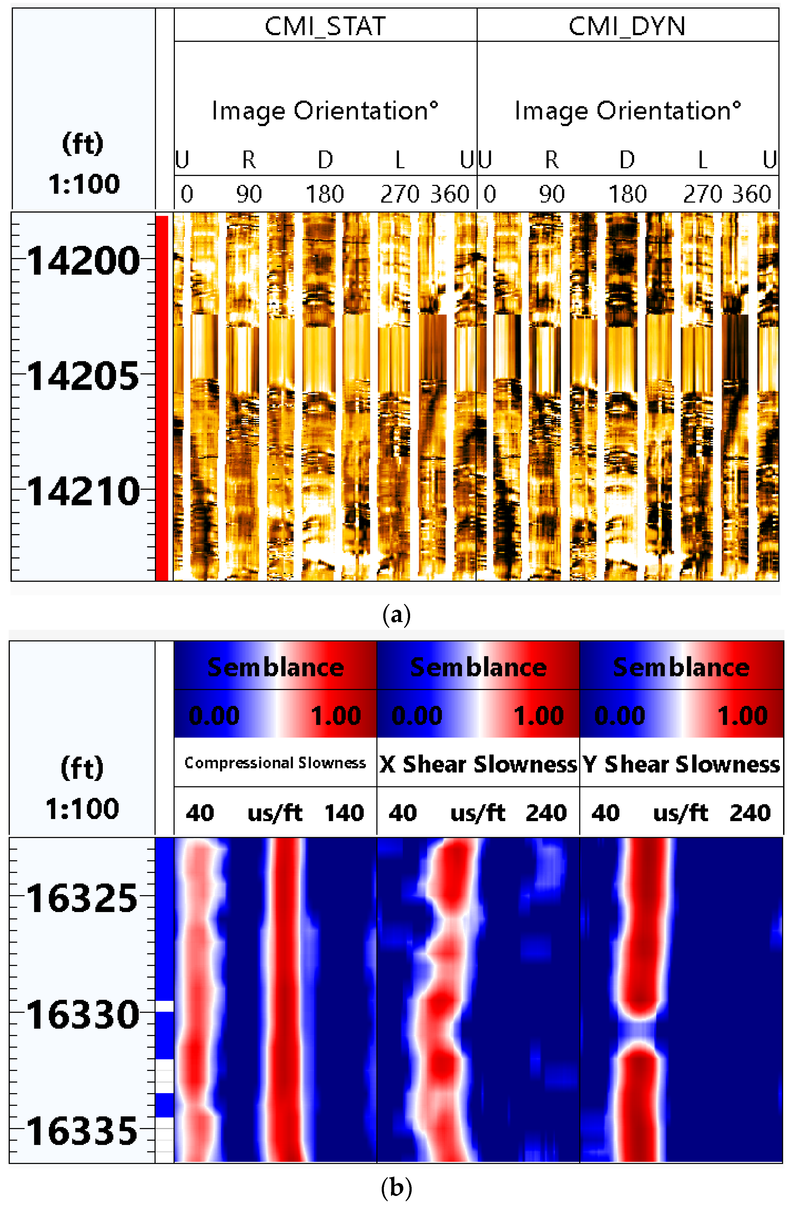
The study well contains triple combo data including gamma ray, raw resistivity image data from an imaging tool and raw waveforms from a dipole acoustic tool as well as a complete suite of logs used for formation evaluation. Image data from a compact micro-imager tool (CMI) and acoustic data from a compact cross-dipole sonic tool (CXD) were processed and interpreted. Several factors can result in poor image quality. Image data were flagged for any image quality issues due to artefacts [14,15] related to drilling such as cuttings’ interference or stick and pull. Acoustic semblance is a measure of the similarity between the waveforms recorded by a borehole acoustic logging tool and a reference waveform; a high acoustic semblance indicates that the recorded waveform is similar to the reference waveform, while a low acoustic semblance indicates that the recorded waveform is dissimilar to the reference waveform [16]. Acoustic data were flagged for any quality issues any time semblance was less than 0.65 due to borehole rugosity or mud cake or various kinds of incoherent and coherent noises. Figure 1 provides examples of image quality issues due to cuttings and stick and pull, and acoustic quality issues due to borehole rugosity.

Table 1. Description of well log data used in the study.

Mnemonic	Curve	Unit	Value Range	Sampling Rate
GMGC	Gamma Ray	API	12.2–289.2	0.5 inches
VSH	Volume of Shale	v/v	0–1	0.5 inches
ANIS	Anisotropy	%	0.0–29.7	0.5 inches
DTFS	Fast Shear Slowness	us/ft	83.3–125.9	0.5 inches
DTSS	Slow Shear Slowness	us/ft	79.8–106.9	0.5 inches
CMI_STAT	Processed Static Resistivity Image	mmho	0–255	0.2 cm
CMI_DYN	Processed Dynamic Resistivity Image	mmho	0 -255	0.2 cm

shows a list of logs used for this study.

A plot of the processed fast and slow shear slowness, anisotropy, and VSH (as a volume fraction, being the ratio of shale solid volume divided by total solid volume, v/v) curves is displayed in Figure 2. The lithological variability of the anisotropy is obvious on the VSH log with clean intervals exhibiting less anisotropy. A histogram of the VSH values (Figure 3) is consistent with the dominance of three lithologies: clean (predominantly calcite), dirty with about 20% volume of clay or shale rich. The mean anisotropy over the interval is 7.1% (Figure 4). Figure 5 shows the processed static and dynamic image data along with fracture interpretations. Resistive fractures are characterized as sinusoidal traces of high resistivity when compared to the resistivity of the surrounding rock matrix. The identified fractures are near vertical with a median dip of 86.2°. Not all fractures will be detected by interpretation of the image log. Furthermore, microfractures will neither be resolved nor detected, though they will clearly affect the shear-wave velocities. For these reasons, the measured fracture counts must be considered only a minimum fracture count. If the microfractures parallel the detected macrofractures, then they will result in additional in situ anisotropy. Conversely, if microfractures are significant, using observed shear-wave anisotropy to estimate fracture counts will thus overestimate the fracture frequency relative to only those observable fractures.

3. Methods

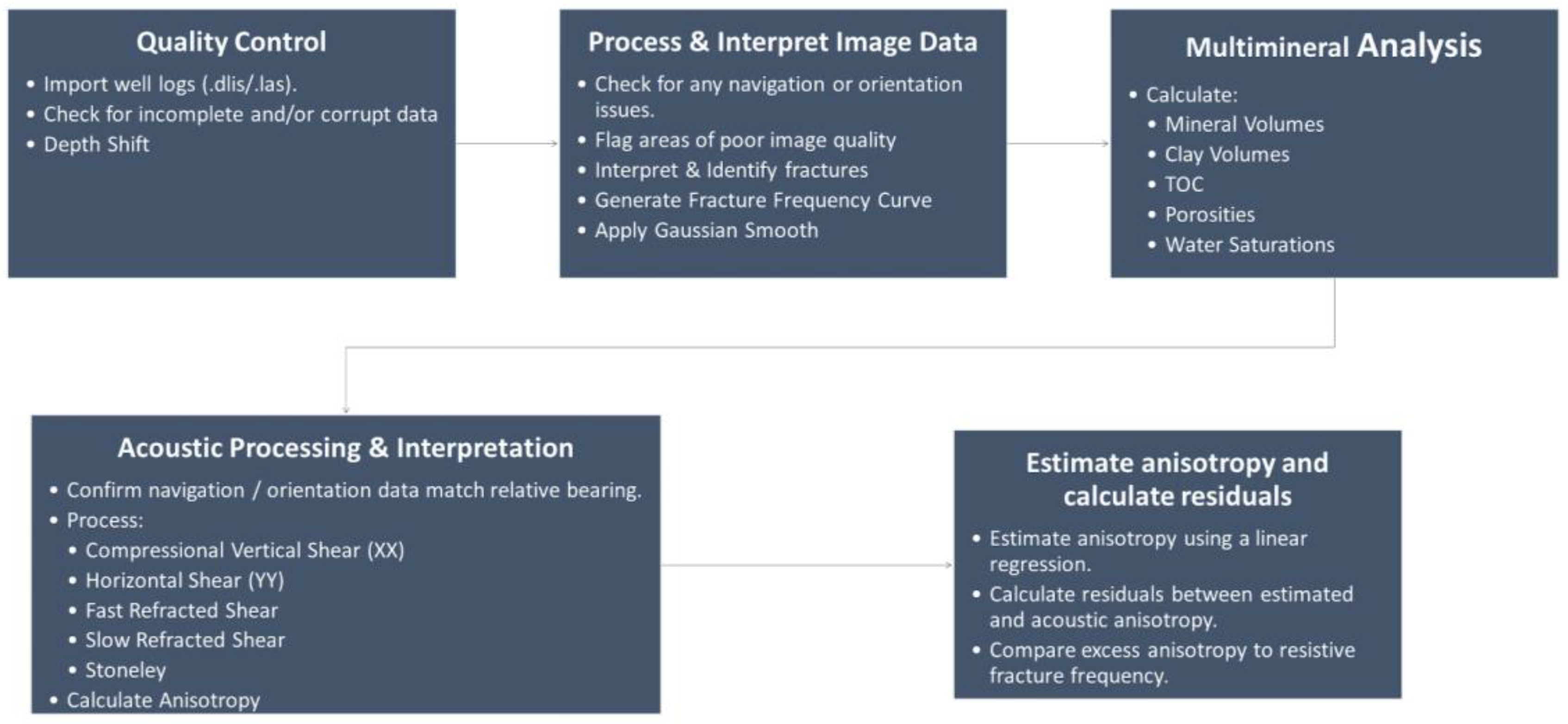
Figure 6 shows the workflow we used to predict the resistive fracture frequency using linear regression and residual anisotropy determination. In summary: The logs are first imported, aligned and checked for completeness, data integrity, navigation and orientation issues, and intervals of poor data quality. The image logs are displayed, fractures identified and fracture counts tabulated. The fracture counts are smoothed with a Gaussian filter (standard deviation of 1.68 feet) to make them more compatible with conventional wireline logs. Multimineral analysis is applied to the conventional well logs to produce mineral volumes (especially volume fraction of shale), total organic carbon, porosities and water saturation. The acoustic log is processed for vertical (oriented along the borehole), compressional and shear-wave velocity, horizontally polarized shear and Stoneley-wave velocity. The shear waves are oriented to produce the fast and slow refracted shear-wave velocities, and these are used to calculate measured anisotropy. Linear regression is applied to predict the measured anisotropy from the volume of shale and residuals are calculated. This excess anisotropy is further smoothed and resampled, and regressed against the fracture counts, producing a regression equation to predict fracture frequency from the excess anisotropy. This equation is applied to the excess anisotropy log to predict frequency.

Fractures were characterized from nearly 5000 feet of oriented horizontal resistivity images through the Delaware Wolfcamp shale. Fractures were classified as resistive, conductive or mixed based on fracture traces. The intensity of fractures was quantified in terms of frequency (number of fractures per foot of image). The number of fractures was counted for a sliding 1-foot boxcar window sampled every foot. An additional fracture frequency curve was created using a Gaussian smoothing operator with a standard deviation of 1.68 feet, for comparison to anisotropy and residual logs of similar resolution.

A static organic mudstone petrophysical analysis and interpretation was performed as outlined by Newsham et al. [17,18,19], and the mineral volumes, shale volumes, TOC, porosity and water saturation were calculated. VSH was recalculated using a cutoff of 85 API to identify shale, and an additional cutoff of 185 to exclude any calculated clay content above 100%. The anisotropy Ԑ, was then computed using the processed fast ($\mathsf{\Delta }{t}_{Fast Shear})$ and slow shear ($\mathsf{\Delta }{t}_{Slow Shear}$) transit-time logs Equation (1).

$$\mathrm{Ԑ}=\frac{\mathsf{\Delta }{t}_{Slow Shear}-\mathsf{\Delta }{t}_{Fast Shear}}{\left(\mathsf{\Delta }{t}_{Slow Shear}+\mathsf{\Delta }{t}_{Fast shear}\right)/2}$$

(1)

The percent anisotropy is linearly related to computed fractional VSH (Figure 7) with a correlation coefficient of 0.6.

The low correlation suggests additional factors contribute to the measured anisotropy. The lithology-related anisotropy can be predicted using a simple linear regression Equation (2):

$${\mathrm{Ԑ}}_{Predicted}=13.30\times VSH+2.87$$

(2)

Despite the low correlation, due to the large number of datapoints, the F-test is a robust F = 4557, indicating that the explained variance is significantly greater than the unexplained variance, with P = 0, indicating that there is zero probability that the correlation is by chance. The root-mean-squared prediction error is 3.3%, suggesting that much of the observed anisotropy can be predicted using this equation, although the cross-plot and low correlation show that much anisotropy is not accounted for. We will use this incomplete prediction to our advantage by hypothesizing that some portion of the anisotropy caused by fractures [10] is not predicted by Equation (2).

Residuals (e) were calculated in Equation (3) by subtracting the predicted anisotropy Equation (2) from the calculated acoustic anisotropy Equation (1) and adding back the intercept in Equation (2) of 2.87 to force most values to have positive excess anisotropy.

$$e= \mathrm{Ԑ}-{\mathrm{Ԑ}}_{Predicted}+2.87$$

(3)

The residuals and fracture counts were then smoothed with a 100 ft Gaussian operator. The smoothed residual is then regressed against the observed relative resistive fracture count frequency, f, in units of fractures per foot, yielding:

f = 0.045e + 0.053

(4)

with a correlation coefficient of 0.66 and a standard error of 0.1 fractures/ft. This regression is also highly statistically significant with F = 184 and a p-test value of 10⁻²⁸.

In order to validate the method of qualitative fracture identification discussed above, the same analysis was performed on a second horizontal well in the Wolfcamp Formation approximately 1.75 miles away from the study well. A total of 574 fractures are identified on the image log over a depth interval of 4582 feet; of these, 474 are classified as resistive. The lithology in the second well is similar to that of the study well, with highly variable mixed carbonate–siliciclastic lithology, variations in TOC and two nearly orthogonal resistive fracture sets, which also result in a highly variable measured anisotropy throughout the formation (from 0.0% to 19.4%). The percentage of swelling clays, specifically, smectite, resulted in poorer image quality in this well, resulting in fewer fractures being identified.

The lithology-related anisotropy was predicted using a simple linear regression from a cross-plot of vshale and dipole acoustic anisotropy (Figure 8) given by Equation (5). Data points that occur within a poor image or acoustic-quality flag were excluded from the remaining data.

$${\mathrm{Ԑ}}_{Predicted}=39.95\times VSH-0.83$$

(5)

Despite a low correlation, the F-test is a robust F = 3459, indicating that the explained variance is significantly greater than the unexplained variance, with P = 0, indicating that there is zero probability that the correlation is by chance. The root-mean-squared prediction error is 3.9%, suggesting that much of the observed anisotropy can be predicted using this equation, although the cross-plot and low correlation show that much of the anisotropy is not accounted for. We will again use this incomplete prediction to our advantage by hypothesizing that some portion of the anisotropy caused by fractures [10] is not predicted by Equation (2).

Residuals (e) were calculated in Equation (3) by subtracting the predicted anisotropy Equation (2) from the calculated acoustic anisotropy Equation (1) and adding back the intercept in Equation (2) of −0.83.

$$e= \mathrm{Ԑ}-{\mathrm{Ԑ}}_{Predicted}-0.83$$

(6)

The difference in coefficients between Equation (5) and those obtained in the first well emphasizes the qualitative nature of the observed relationship between lithology and intrinsic anisotropy as well as differences in data quality. Consequently, even with local calibration, we believe that the proposed method can, at best, be expected to qualitatively indicate relative changes in anisotropy residuals and resulting predicted fracture frequency, rather than absolute numbers.

The residuals and fracture counts were then smoothed with a 100 ft Gaussian operator. The smoothed residual is then regressed against the observed relative resistive fracture count frequency, f, in units of fractures per foot, yielding:

$$f=4.26e+11.65$$

(7)

with a correlation coefficient of 0.71 and a standard error of 0.1 fractures/ft. This regression is also highly statistically significant with F = 172 and a p-test value of 0.

4. Results and Discussion

The predicted and observed anisotropy for the first well are plotted in track four of Figure 9. This figure shows that shale-rich and highly interbedded intervals have higher anisotropy, while clean massive intervals have low anisotropy. The residual anisotropy, due in part to in situ anisotropy, in track 5 visually correlates to the resistive fracture count (both quantities smoothed as discussed above)—suggesting that the resistive fractures contribute to the observed anisotropy, but that this has not been accounted for in the predicted anisotropy using the VSH log, which partially accounts for the intrinsic anisotropy due to the shale content. The in situ anisotropy, due in part to the natural fractures, is thus correlated to the residual anisotropy calculation. Figure 10 shows the positive correlation in this well, with a correlation coefficient of 0.661 between the residuals and the resistive fracture frequency.

The predicted and observed anisotropy for the validation well are plotted in track four of Figure 11. This figure shows that shale-rich and highly interbedded intervals have higher anisotropy, while clean massive intervals have low anisotropy. The residual anisotropy, due in part to in situ anisotropy, in track 5 visually correlates to the resistive fracture count (both quantities smoothed as discussed above)—suggesting that the resistive fractures contribute to the observed anisotropy, but that this has not been accounted for in the predicted anisotropy using the VSH log, which partially accounts for the intrinsic anisotropy due to the shale content. The in situ anisotropy, due in part to the natural fractures, is thus correlated to the residual anisotropy calculation. Figure 12 shows the positive correlation, with a correlation coefficient of 0.9 between the residuals and the resistive fracture frequency.

5. Conclusions

(1)

We find VSH to be a strong predictor of anisotropy, and the residual in that estimate relative to cross-dipole-measured anisotropy is a predictor of resistive fracture frequency in these horizontal wells;

(2)

Applying this method to determine the presence of fractures using only the computed VSH and cross-dipole sonic logs has the potential to provide a rough estimate of relative fracture frequency when image logs are not available, and allows for a better understanding of seismic-wave propagation in anisotropic formations;

(3)

This method can potentially speed up fracture-analysis response time, and has the potential to be used not only as an answer product for wireline customers but as a live answer product for logging while drilling (LWD) customers and for calibration of relative fracture intensity predictions from seismic data when image logs are not available.

References

1. Kvale, E.P.; Bowie, C.M.; Flenthrope, C.; Mace, C.; Parrish, J.M.; Price, B.; Anderson, S.; DiMichele, W.A. Facies variability within a mixed carbonate-siliciclastic sea-floor fan (upper Wolfcamp Formation, Permian, Delaware Basin, New Mexico). AAPG Bull. 2020, 104, 525–563. [Google Scholar] [CrossRef]
2. Salem, A.C.; Naruk, S.J.; Solum, J.G. Impact of natural fractures on production from an unconventional shale: The Delaware Basin Wolfcamp shale. AAPG Bull. 2022, 106, 1–20. [Google Scholar] [CrossRef]
3. Cortez, M. Chemostratigraphy, Paleoceanography, and Sequence Stratigraphy of the Pennsylvanian—Permian Section in the Midland Basin of West Texas, with Focus on the Wolfcamp Formation. Master’s Thesis, University of Texas at Arlington, Arlinton, TX, USA, 2012. [Google Scholar]
4. Forand, D.; Heesakkers, V.; Schwartz, K. Constraints on natural fracture and in-situ stress trends of unconventional reservoirs in the Permian Basin, USA. In Proceedings of the SPE/AAPG/SEG Unconventional Resources Technology Conference 2017, Austin, TX, USA, 24–26 July 2017. [Google Scholar] [CrossRef]
5. Fernández-Ibáñez, F.; DeGraff, J.M.; Ibrayev, F. Integrating borehole image logs with core: A method to enhance subsurface fracture characterization. AAPG Bull. 2018, 102, 1067–1090. [Google Scholar] [CrossRef]
6. Guo, T.; Wang, H.; Guo, Y.; Zhang, J.; Jiang, M.; Chen, P.; Kong, X. Fracture Prediction based on an Improved Anisotropy Inversion: A Shale Reservoir Fracture Prediction Case Study. In SEG Technical Program Expanded Abstracts; Society of Exploration Geophysicists: Houston, TX, USA, 2019; pp. 414–418. [Google Scholar] [CrossRef]
7. Pollock, C.; Seiler, C.; Valcárcel, M.; Macaulay, E. A method of fracture prediction across multiple stratigraphic horizons in the Midland Basin, Texas, USA. In Proceedings of the SPE/AAPG/SEG Unconventional Resources Technology Conference 2018 (URTC 2018), Houston, TX, USA, 23–25 July 2018. [Google Scholar] [CrossRef]
8. Thomsen, L. Weak Elastic Anisotropy. Geophysics 1986, 51, 1954–1966. [Google Scholar] [CrossRef]
9. Tsvankin, I.; Gaiser, J.; Grechka, V.; van der Baan, M.; Thomsen, L. Seismic anisotropy in exploration and Reservoir Characterization; an Overview. Geophysics 2001, 75, 75A15–75A29. [Google Scholar] [CrossRef] [Green Version]
10. Jian, S.; Fu, L.; Cheng, Y. Anisotropic effective elastic properties for multi-dimensional fractured models. Appl. Sci. 2022, 12, 1873. [Google Scholar] [CrossRef]
11. Saxena, V.; Krief, M.; Adam, L. Borehole Acoustic Logging. In Handbook of Borehole Acoustics and Rock Physics for Reservoir Characterization; Elsevier: Amsterdam, The Netherlands, 2018; pp. 43–85. [Google Scholar] [CrossRef]
12. Vernik, L.; Milovac, J. Rock physics of organic shales. Lead. Edge 2011, 30, 318–323. [Google Scholar] [CrossRef]
13. Vernik, L. Microcrack-induced versus intrinsic elastic anisotropy in mature HC-source shales. Geophysics 1993, 58, 1703–1706. [Google Scholar] [CrossRef]
14. Lofts, J.C.; Bourke, L.T. The recognition of artefacts from acoustic and resistivity borehole imaging devices. Geol. Soc. Lond. Spec. Publ. 1999, 159, 59–76. [Google Scholar] [CrossRef]
15. Cheung, P.S. Microresistivity and ultrasonic imagers: Tool operations and processing principles with reference to commonly encountered image artefacts. Geol. Soc. Lond. Spec. Publ. 1999, 159, 45–57. [Google Scholar] [CrossRef]
16. Paillet, F.L.; Dellinger, J.G. Cross-dipole acoustic anisotropy measurements: Interpretation and applications. Dev. Pet. Sci. 2017, 68, 329–383. [Google Scholar]
17. Newsham, K.; Comisky, J.; Chemali, R. Organic-Mudstone Petrophysics: Workflow to Estimate Storage Capacity. Petrophysics 2019, 60, 4–15. [Google Scholar] [CrossRef]
18. Newsham, K.; Comisky, J.; Chemali, R. Organic mudstone petrophysics, Part 2: Workflow to estimate storage capacity. Petrophysics 2019, 60, 181–207. [Google Scholar] [CrossRef]
19. Newsham, K.; Comisky, J.; Chemali, R. Organic mudstone petrophysics, Part 3: Workflow to estimate storage capacity. Petrophysics 2019, 60, 351–371. [Google Scholar] [CrossRef]
Figure 1. Examples of (a) image quality issues due to stick and pull along with cuttings interference causing an image quality where bedding is visible, but fracture identification is difficult, and (b) acoustic quality issues due to borehole rugosity and mud cake.
Energies 16 02838 g001
Figure 2. Well logs and observed shear-wave anisotropy. Track 1 shows the image caliper log relative to the bit size and poor acoustic- and image quality flags. VSH in the center track (with units of volume fraction) has color fill of the VSH values with lower VSH in lighter colors (mostly carbonates) and higher VSH values in darker colors (shales). The next track to the right contains the anisotropy curve in blue calculated from measured velocities. The rightmost track contains the processed fast shear (red curve) and slow shear (blue curve) slowness curves used to calculate the anisotropy.
Energies 16 02838 g002
Figure 3. Histogram of VSH values (v/v) over the study well (x-axis), frequencies (left y-axis) and cumulative frequencies (right y-axis and black curve) A number of dominant lithologies are apparent, including clean carbonates (VSH less than 0.1), dirty limestones (VSH from 0.15 to 0.25), shales (VSH above 0.25) and clay-rich shales (VSH above 0.7). The shales with low VSH indicate high quartz content in the fine-grained fraction.
Energies 16 02838 g003
Figure 4. Histogram of absolute value of percent anisotropy (using Equation (1)) over the study well (x-axis), frequencies (left y-axis) and cumulative frequencies (right y-axis and black curve). Most shales have anisotropy greater than 5%.
Energies 16 02838 g004
Figure 5. Portion of the static wellbore resistivity image within the Wolfcamp (bottom track) with overlain fracture interpretation (middle track) and fault dip and strike (third track) using fracture dip symbols to display the direction of strike and dip. The dip angle can be determined by the location of the dip symbol in the track (0–90°).
Energies 16 02838 g005
Figure 6. Suggested workflow for fracture frequency prediction starting with quality control of well logs, processing, interpretation and evaluation of data, followed by the linear estimation of anisotropy and calculation of residuals.
Energies 16 02838 g006
Figure 7. Cross-plot showing VSH in v/v units (x-axis) and dipole acoustic anisotropy in percent (y-axis). The cross-plot is colored by VSH values, with lower values in the lighter colors (carbonates) and higher values in the darker colors (shales). The sample size of the dataset (nb) is 8697 datapoints. The correlation (R) between the predictor variable VSH and the response variable anisotropy is 0.602.
Energies 16 02838 g007
Figure 8. Cross-plot showing VSH in v/v units (x-axis) and dipole acoustic anisotropy in percent (y-axis) in a second well. The cross-plot is colored by VSH values, with lower values in the lighter colors (carbonates) and higher values in the darker colors (shales). The sample size of the dataset (nb) is 4547 datapoints. The correlation (R) between the predictor variable VSH and the response variable anisotropy is 0.660.
Energies 16 02838 g008
Figure 9. Plot showing a strong correlation in the first well between the cross-dipole sonic anisotropy (CXD) and the anisotropy predicted using Equation (2), and a strong correlation between the residuals and resistive fracture frequency when smoothed with a 100 ft Gaussian operator. The first track to the right of depth displays the caliper data colored by the mud cake (tan)/washout (aquamarine), along with the image quality flags (red) and acoustic quality flags (blue). The black curve, in the third track, is the volume of shale (VSH) log showing obvious lithological variability. The blue curve, in the fourth track, is the dipole acoustic anisotropy. The pink curve, in the fourth track, is the predicted anisotropy using Equation (3). The fifth track contains the calculated residuals in purple and the resistive fracture frequency in black.
Energies 16 02838 g009
Figure 10. Cross-plot in the first well showing residuals (difference between the dipole acoustic anisotropy and the calculated anisotropy) on the (x-axis) and resistive fracture frequency (y-axis), after resampling at 25 feet. The cross-plot is colored by VSH (shale volume fraction) values, with lower values in the lighter colors (carbonates) and higher values in the darker colors (shales). The sample size of the dataset (nb) = 166. The correlation (R) between the predictor variable VSH and the response variable anisotropy is 0.66.
Energies 16 02838 g010
Figure 11. Well logs from the validation well showing a strong correlation between the cross-dipole sonic anisotropy (CXD) and the anisotropy predicted using Equation (5), and a strong correlation between the residuals and resistive fracture frequency when smoothed with a 100 ft Gaussian operator. The first track to the right of depth displays the caliper data colored by the mud cake (tan)/washout (aquamarine), along with the image quality flags (red) and acoustic quality flags (blue). The black curve, in the third track, is the volume of shale (VSH) log showing obvious lithological variability colored by VSH values, with lower values in the lighter colors (carbonates) and higher values in the darker colors (shales). The blue curve, in the fourth track, is the dipole acoustic anisotropy. The pink curve, in the fourth track, is the predicted anisotropy using Equation (6). The fifth track contains the calculated residuals in purple and the resistive fracture frequency in black.
Energies 16 02838 g011
Figure 12. Cross-plot from the validation well showing residuals (difference between the dipole acoustic anisotropy and the calculated anisotropy) on the (x-axis) and resistive fracture frequency (y-axis), after resampling at 25 feet. The cross-plot is colored by VSH (shale volume fraction) values, with lower values in the lighter colors (carbonates) and higher values in the darker colors (shales). The sample size of the dataset (nb) = 166. The correlation (R) between the predictor variable VSH and the response variable anisotropy is 0.9.
Energies 16 02838 g012