Quantitative Prediction of Braided Sandbodies Based on Probability Fusion and Multi-Point Geostatistics

Abstract

Predicting the spatial distribution of braided fluvial facies reservoirs is of paramount significance for oil and gas exploration and development. Given that seismic materials enjoy an advantage in dense spatial sampling, many methods have been proposed to predict the reservoir distribution based on different seismic attributes. Nevertheless, different seismic attributes have different sensitivities to the reservoirs, and informational redundancy between them makes it difficult to combine them effectively. Regarding reservoir modeling, multi-point geostatistics represents the distribution characteristics of the braided fluvial facies reservoirs effectively. Despite this, it is very difficult to build high-quality training images. Hence, this paper proposes a three-step method of predicting braided fluvial facies reservoirs based on probability fusion and multi-point geostatistics. Firstly, similar statistical data of modern sedimentation and field paleo-outcrops were processed under the guidance of the sedimentation pattern to construct reservoir training images suitable for the target stratum in the research area. Secondly, each linear combination of selected seismic attributes was demarcated to calculate the principal component value and work out the elementary conditional probability. Lastly, the PR probability integration approach was employed to combine all conditional probabilities and calculate the joint probability. Then the joint probability was combined with training images to build a reservoir distribution model through multi-point geostatistics. We illustrated the detailed workflow of our new method by applying it to a braided fluvial reservoir modeling case in the Bohai Bay Basin, East China. The new method reduced the error of prediction results by 32% and 46% respectively, and the error of water content by 36.5% and 60.3%. This method is a potentially effective technique to predict and characterize the reservoir spatial distribution and modeling in other oil fields with the same geological background.

1. Introduction

The braided fluvial facies sand is one of the critical types of oil-gas reservoirs [1]. Due to frequent swings of river channels, it is characterized by multi-stage superposition, complex temporal–spatial distribution, and high heterogeneity [2,3]. In addition, channel sand directly controls the distribution of reservoir properties (including porosity and permeability). Therefore, predicting the spatial distribution of braided fluvial facies sand is significant for exploring and developing underground oil and gas. Furthermore, it is a critical topic studied by geophysicists and petroleum geologists [4,5,6]. Generally speaking, petroleum geologists predict reservoir sand through cores, logs, and seismic data [7,8,9]. Although core identification is the most direct method, it is confined to the targeted stratum and is time-consuming and pricy. Thus, it is crucial to predict the spatial distribution of braided fluvial facies sand with logs and seismic data. If the braided fluvial sand is in oilfields with a dense well pattern, its spatial distribution characteristics can be predicted with diverse interpolation methods based on logging data [10,11]. For oilfields with 3D seismic data, the spatial distribution of the reservoir can be effectively predicted based on seismic attributes [12,13].

Various processing techniques based on seismic data have been widely applied to predicting the spatial distribution, lithological distribution, and physical properties of underground reservoirs [7,14,15]. For instance, seismic amplitude data, frequency data, and seismic inversion data have been extensively used to predict reservoirs’ spatial distribution [16,17,18,19,20]. However, seismic data are characterized by a low vertical resolution rate, strong multiplicity, the tuning effect, and high uncertainty in one-dimensional borehole data, making it hard to predict braided fluvial facies sand with fast plane facies change and strong heterogeneity effectively [18,21,22,23,24,25].

In recent years, methods that predict fluvial reservoirs with multiple types of seismic data have been widely applied and developed to overcome the defect of high uncertainty in a single seismic attribute [8,18,22,23,25]. Some scholars employ the continuous wavelet transform [26], the Fourier Transform [15], and other spectrum decomposition techniques to break down primary seismic data into a series of seismic data with different frequencies, from which they select seismic data with the appropriate frequency for predicting the distribution of fluvial facies reservoirs. On this basis, some scholars proposed the RGB method in which red, green, and blue stand for seismic attributes with low, medium, and high frequencies [27,28,29,30]. Specifically, the mapping function converts three input colors proportionately and eventually gets an RGB blended color value that corresponds to each point to predict the fluvial facies reservoir’s boundary [4,5]. In addition, methods, including the clustering methodology and multiple linear regression are also employed to predict the fluvial reservoir.

However, the methods mentioned above face deficiencies in predicting fluvial facies reservoirs. Although the spectrum analysis obtains several data volumes with a narrow spectrum, the single data volume is devoid of many effective frequencies. The RGB method is essentially a multiple linear regression model [5,26], but the relations between the sandbody thickness and seismic attributes with different frequencies are non-linear and are unable to pass the RGB’s optimal regression model. Moreover, the RGB’s fused attributes are the output of three input colors and reflect only the sandbody’s distribution laws rather than quantitatively representing the sandbody’s distribution. In addition, the RGB method only receives three input values at maximum and becomes inapplicable when seismic attributes exceed three. Similarly, the clustering method achieves clustered plane facies, which fail to represent the sandbody’s distribution quantitatively. The multiple linear regression method is restricted by sensitive attributes, so attribute optimization profoundly affects the prediction accuracy.

The probability fusion method receives growing attention because it predicts research objectives quantitively with several types of data. As of yet, this method has been extensively applied to and made headway in fields including single-well lithology identification [31] and fracture prediction [32]. The probability fusion method mainly consists of the PR model, Tau model, and λ model [31,32,33]. A significant effect has been made in combining several types of data with the probability fusion method. Auxiliary data are assumed to be independent [33], but in fact, they tend to be correlated and contradict the independence hypothesis. In addition, the unquantifiable redundancy between basic data results in a severe deviation in the fused probability bodies. On this basis, Yuming Liu et al. (2020) [32] proposed an improved probability fusion method based on PCS and the PR model to avoid deviations caused by redundancy between the elementary data effectively and this method has been successfully applied to fracture prediction and modeling. However, the method has its deficiencies and fails to apply the fracture development pattern to fracture prediction. In reality, the development pattern plays a critical role in controlling the fracture distribution and serves as an essential knowledge source for reducing the uncertainties in the fracture’s spatial distribution. Meanwhile, scant literature mentions predicting the braided fluvial facies reservoir with the probability fusion method [31,34,35,36]. Therefore, this paper proposed a three-step method for predicting braided fluvial facies reservoirs. Firstly, measurement statistics of modern sedimentation and field paleo-outcrops were combined with cores and logging data to construct training images suitable for the reservoir in the research area under the sedimentation pattern’s constraints. 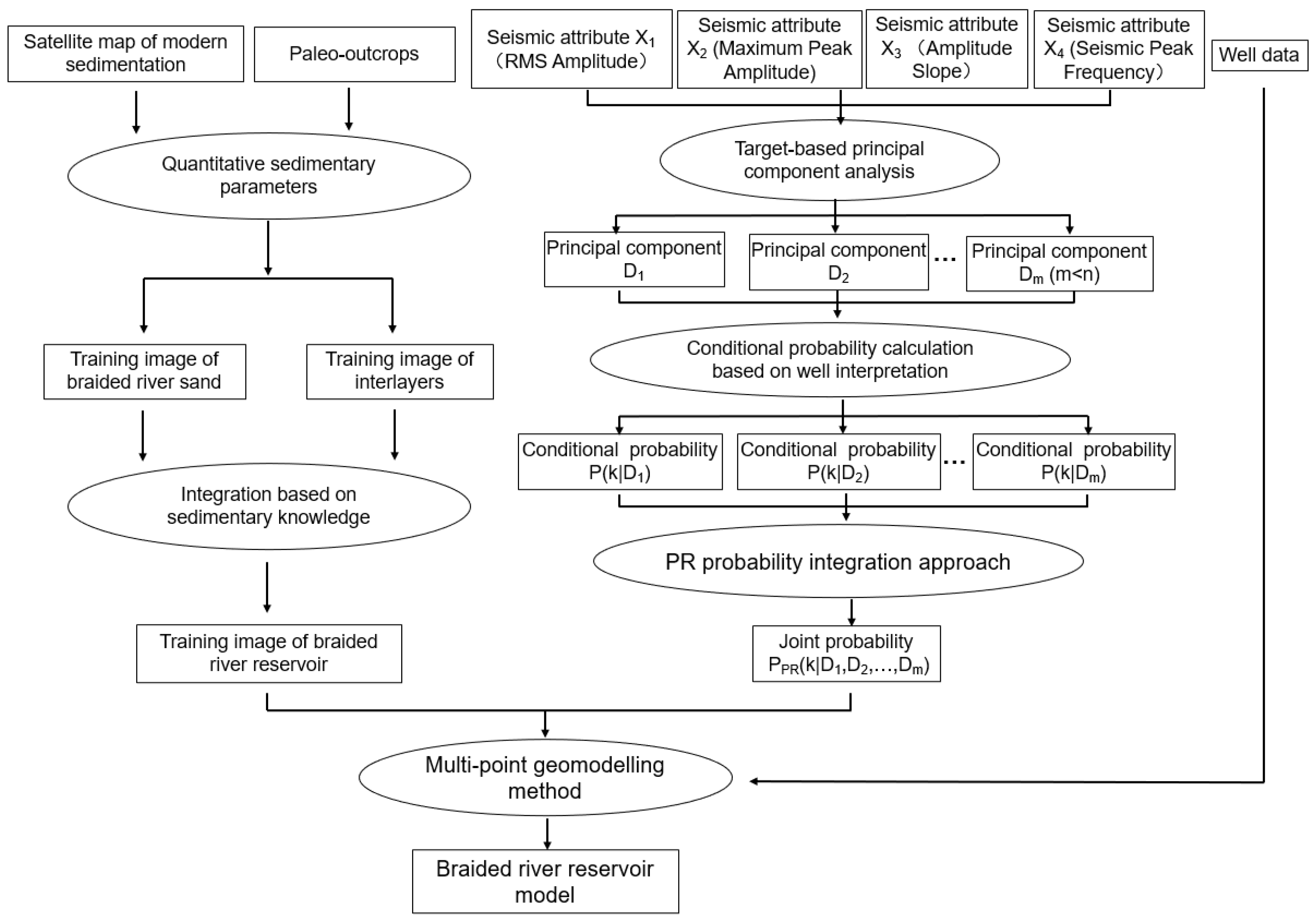Secondly, the PCA method was employed to convert the sensitive seismic attribute data into a group of independent principal components [37,38,39]. In the PCA progress, each seismic attribute was given a weight based on the correlation coefficient between seismic attributes and the sand, and principal components were selected based on the correlation coefficients between their values with the sand thickness and the accumulative contribution rate. Afterward, the elementary conditional probability was obtained by calibrating the correlation between the principal component value and sand development probability on the well. Finally, the PR model was employed to combine several conditional probabilities into one joint probability, and we could establish the spatial distribution model for the braided fluvial facies reservoir by using the joint probability volume and training image under the Sneisim algorithm of multi-point geostatistics.

2. Materials and Methods

2.1. Materials

The dataset that was used to predict the braided fluvial facies reservoir and establish models in this paper includes 46 wells in the Zhaodong Oilfield in the Bohai Bay Basin of China. The target layer in the paper is on the upper Neogene Guantao Formation. Its overall structure is high in the north yet low in the south, with a formation thickness of 250–373 m. The provenance originates from the Chengning Uplift in the south and falls into the category of braided fluvial facies deposits. One well in the study area was cored, most of these wells have abundant well logs, including spontaneous potential (SP), sonic (AC), deep laterolog (Rd), shallow laterolog (Rs), and density (DEN) logs, and all of these wells also have facies interpretations. The Zhaodong Oilfield is covered with a 3D seismic cube, which shows a dominant frequency of 34 Hz and a bandwidth of 21–56 Hz. In addition, 21 typical braided river modern sedimentations and 5 field paleo-outcrops were statistically studied to establish the reservoir prediction model.

2.2. Method

This paper proposed a three-step method for predicting fluvial braided facies reservoirs: (1) construct training images suitable for the target stratum with statistical methods based on measurement data of modern sedimentation and paleo-outcrops; (2) employ the object-oriented PCA to calculate the conditional probability volume for reservoir development based on seismic attributes; (3) combine conditional probabilities with the probability fusion method and construct the reservoir distribution model with multi-point geostatistics. The basic workflows of the proposed method are shown in Figure 1, and relevant details are introduced in the following three sections.

2.2.1. Construction of Training Image

Compared with traditional two-point geostatistics, multi-point geostatistics reappears the object’s geometrical shapes more effectively. Training images considerably affect the final prediction results; in fact, obtaining quality training images is a challenge. Similarly, modern sedimentation displays the plane geometrical shapes of braided fluvial facies reservoirs visually yet represents the interlayers of reservoirs less efficiently. For another, field paleo-outcrops enjoy a huge advantage in depicting the interlayers. For this reason, this paper proposed a method that constructs training images for fluvial facies reservoirs based on combining modern sedimentation and field paleo-outcrops statistics.

Firstly, the reservoir’s dimensions (length and width) and geometrical shapes were collected through modern sedimentation statistics. Details of the measurement method are presented in Figure 2. Meanwhile, relevant measurement data were processed to establish a quantitative relationship with braided fluvial facies reservoirs and construct prototype training images for braided fluvial facies reservoirs.

Secondly, the thickness and width of different interlayers in the paleo-outcrops were measured to establish the relationships between the dimensional parameters of different interlayers. Details of the measurement method are presented in Figure 3. Next, these relationships were employed to construct prototype training images of interlayers in the braided fluvial facies reservoir.

The constructed initial training images for the reservoirs and their internal interlayers were combined and modified to construct final training images under the sedimentation pattern’s constraints.

2.2.2. Construction of Elementary Conditional Probabilities

The probability fusion method effectively combines a variety of seismic attributes and quantitatively predicts the target with probability. Hence, constructing an elementary probability based on seismic attributes lays a foundation for the probability fusion. However, the information redundancy between different seismic attributes fails to meet the applicable conditions of probability fusion. Therefore, it was not viable to obtain elementary conditional probabilities by demarcating seismic attributes. This problem could be effectively solved through the object-based PCA method. Specifically, the seismic attributes sensitive to the reservoir development underwent the PCA to generate a group of independent principal component data that meets the hypothetical conditions for probability fusion. On this basis, the principal components were optimized based on the accumulative contribution rate and correlation coefficients. Lastly, the correlations between the principal component value and the on-well sandbody development probability were demarcated to construct the elementary conditional probability. The specific workflows of this method are listed as follows:

(1)

Optimize seismic attributes sensitive to the reservoir development based on the correlation coefficient;

(2)

Standardize optimized seismic attributes to ensure they meet the distribution with a mean of 0 and variance of 1, which are denoted as vector X_i (i = 1,….n);

(3)

Determine the weight based on the correlation coefficient between each standardized seismic attribute and sand thickness. Work out the weighted data through Equation (1):

$${\mathrm{X}}_{\mathrm{i}}^{*}={\mathsf{\omega }}_{\mathrm{i}}{\mathrm{X}}_{\mathrm{i}}=(1+\frac{\left|{\mathrm{r}}_{\mathrm{i}}\right|-\left|{\mathrm{r}}_{\min }\right|}{\left|{\mathrm{r}}_{\max }\right|-\left|{\mathrm{r}}_{\min }\right|}{)\mathrm{X}}_{\mathrm{i}}$$

(1)

where variable X_i^* represents the weighted data of the ith standardized seismic attribute; X_i is the ith standardized seismic attribute; ω_i is the weighted coefficient of the ith standardized seismic attribute; r_i is the correlation coefficient between the ith standardized seismic attribute and sand thickness; r_min is the minimum correlation coefficients between the standardized seismic attribute and sand thickness; and r_max is the maximum correlation coefficient between the standardized seismic attribute and sand thickness.

(4)

Calculate the covariance matrix and work out the characteristic vector and characteristic value;

(5)

Calculate the correlation coefficient between each principal component and the on-well sand development probability;

(6)

Select a subset of principal components based on correlation coefficients and the cumulative contribution contents;

(7)

Demarcate the principal components optimized based on the on-well sandbody’s development probability and calculate the elementary conditional probability.

2.2.3. Integration of Elementary Conditional Probabilities and Modeling

The elementary conditional probabilities are independent and meet the hypothesis of probability fusion. Hence, the joint probability can be directly calculated through the PR model [28]. The calculation formula is listed as follows:

$${\mathrm{P}}_{\mathrm{PR}}{\left(\mathrm{k}\right|\mathrm{D}}_1{,\dots ,\mathrm{D}}_{\mathrm{n}})=\frac{{(\frac{1-\mathrm{P}\left(\mathrm{k}\right)}{\mathrm{P}\left(\mathrm{k}\right)})}^{\mathrm{n}-1}}{{(\frac{1-\mathrm{P}\left(\mathrm{k}\right)}{\mathrm{P}\left(\mathrm{k}\right)})}^{\mathrm{n}-1}+{{\displaystyle \prod }}_{\mathrm{i}=1}^{\mathrm{n}}(\frac{{1-\mathrm{P}\left(\mathrm{k}\right|\mathrm{D}}_{\mathrm{i}})}{{\mathrm{P}\left(\mathrm{k}\right|\mathrm{D}}_{\mathrm{i}})})}$$

(2)

where P_PR(k|D₁,…D_n) is the joint conditional probability of target k’s development calculated with the PR model under joint constraints of n types of basic data; P(k) is the global proportion of object k to the development of the whole area; P(k|D_i) is the conditional probability of target k’s development under constraints of ith elementary data; n is the total number of basic data.

After obtaining the training image and joint probability, we could construct the 3D reservoir model under the multi-point geostatistics Snesim algorithm.

3. Results

We illustrate the detailed workflow of the new method by applying it to a braided fluvial reservoir modeling case in the Bohai Bay Basin.

Zhaodong Oilfield is located in the Zhaobei step-fault zone in the southeastern margin of Huanghua Depression, Bohai Bay Basin, East China. It faces the Zhaobei Fault in the south, Zhangdong Fault in the north, and Yangsanmu Uplift in the west [32]. Located in the south of the Zhaodong Oilfield, the research area covered 12 km² and had developed 8 faults (Figure 4).

The target stratum had developed the channel bar, braided river channel, and overflow facies. Its lithology contained conglomerate, medium sandstone, fine sandstone, siltstone, and mudstone. The medium and fine sandstones were primary lithological components of the research area, and its profile reflected the typical sedimentary structures of braided rivers, including trough cross-bedding, sphenoid cross-bedding, and parallel bedding. The rock types included debris-arkosic sandstone and feldspar lithic sandstones, as well as a small amount of arkose sandstone with low compositional maturity. The target interval had an average porosity of 30.12% and a permeability of 1696.23 mD. As a quality reservoir, it enjoys a high untapped potential. However, the reservoir was formed based on channel deposits, and frequent riverway swings result in complicated spatial distribution characteristics and a strong heterogeneity. Thus, predicting the spatial distribution of reservoirs is not only the key to exploring and developing such oil deposits, but is also a complicated problem that should be tackled by oilfields urgently.

3.1. The Training Image

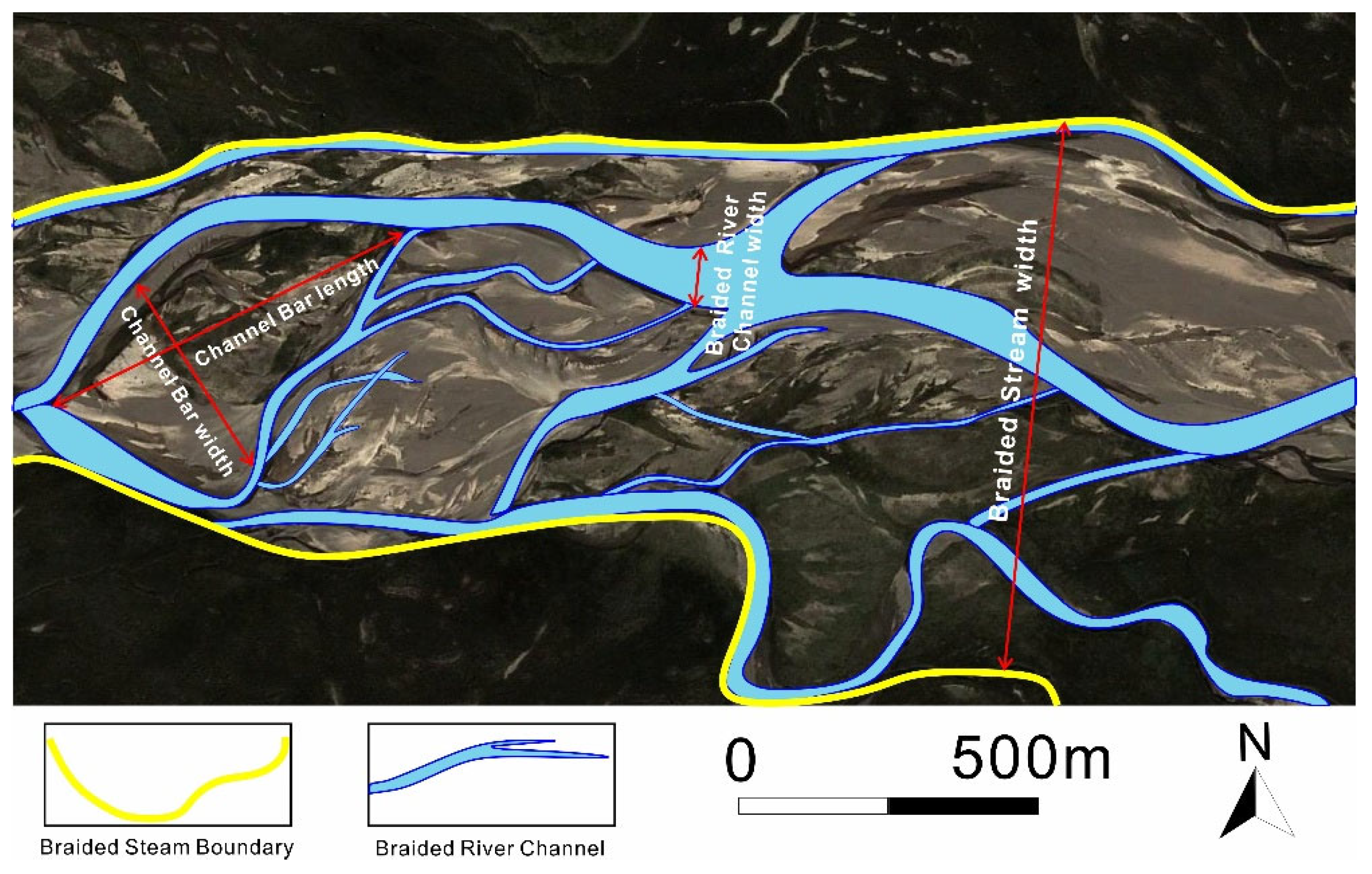
Modern sedimentation is the most effective method for reappearing the sedimentary process in geological history because it vividly displays the plane geometrical forms of braided fluvial deposits. The measurement statistics of modern sedimentation provide a critical basis for quantitively predicting the reservoir scale underground. The target interval studied by the research team consists of sandy braided fluvial facies deposits. Therefore, this paper employed Google Earth to measure the width and length of the channel bar in nine modern sandy braided rivers, including the Yarlung Zangbo River, the Jamuna River, and the Lankaia River in New Zealand, as well as the single riverway width, the braided stream width, the single channel width, and the single channel length. 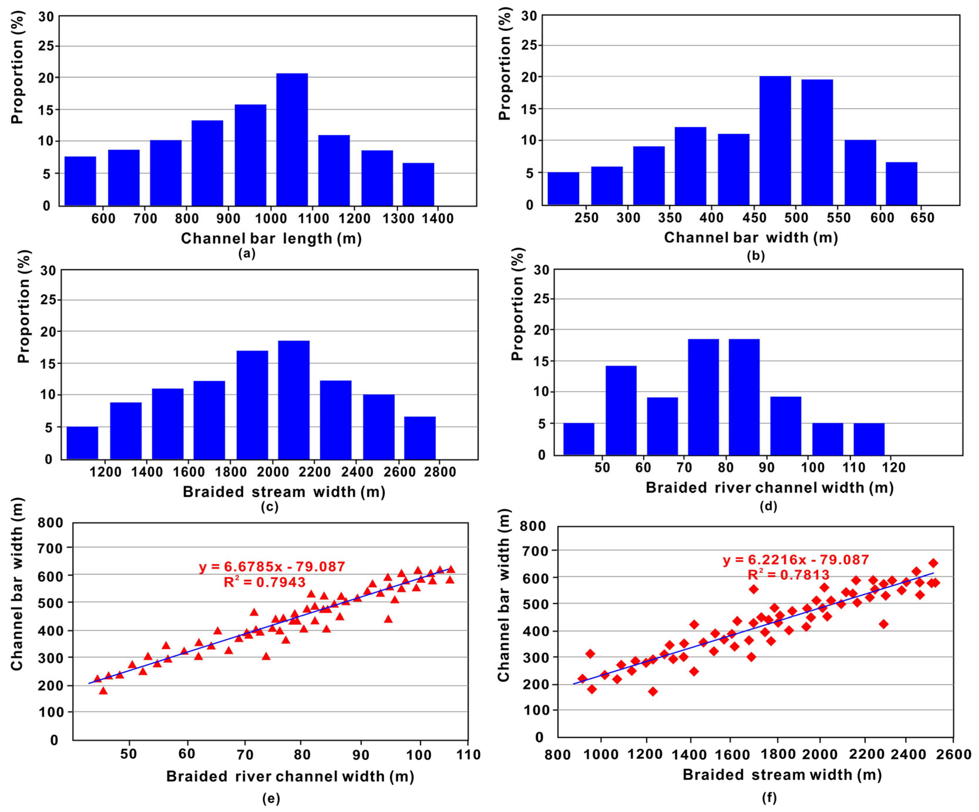Next, these data were processed to establish quantitative relationships between the braided reservoir scales (Figure 5).

The minimum and maximum of the braided stream width were 952 m and 2512 m, with a mean value of 1845 m (Figure 5c). The channel bar’s width was 223–604 m and averaged at 406 m (Figure 5b). The channel bar’s length ranged from 506 m to 1328 m, with an average of 823 m (Figure 5a). The braided river channel width was smaller and ranged from 44.6 m to 103.5 m, with an average of 68 m (Figure 5d). It was found through the statistical fitting between different parameters that the channel bar width was 0.44 times its length, 6.68 times the braided riverway width, and 0.22 times the braided stream width (Figure 5e,f).

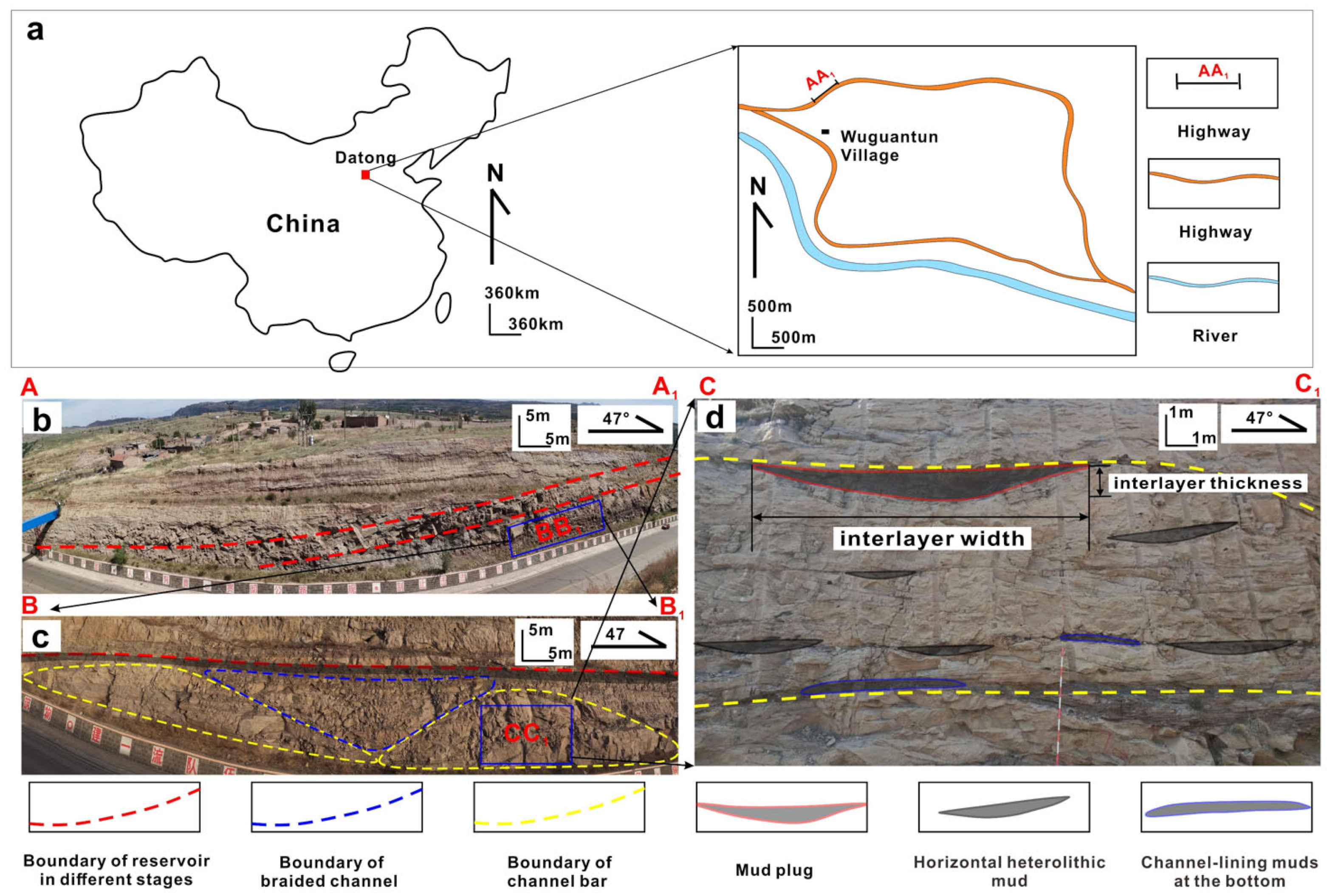
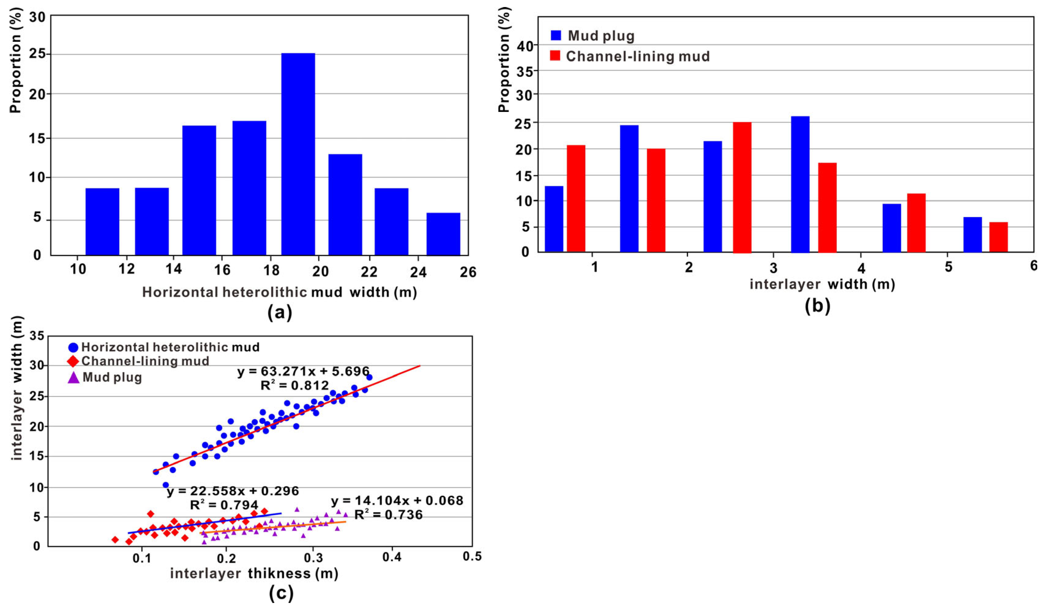
The reservoirs of braided streams are highly heterogeneous, and their interiors consist of mud plugs, horizontal heterolithic mud, and channel-lining muds at the bottom. Different interlayers vary widely in form, scale, and spatial distribution. Although the statistical analysis of modern sedimentation measures the geometrical forms and plane parameters of the channel bar and braided streams visually, it fails to represent interlayers in the reservoirs effectively. On the contrary, the field paleo-outcrop represents the scale and distribution characteristics of interlayers effectively. Therefore, an on-site investigation of sedimentary paleo-outcrops in four typical braided river facies was conducted in Datong, Shanxi, to measure the thickness and width of different interlayers in the reservoirs of braided rivers. Next, the study established correlations between the scale parameters of different interlayers. Specifically, the horizontal heterolithic mud’s width is 63.5 times its thickness; the mud plug’s width is 14 times its thickness; and the channel-lining mud has a width–thickness ratio of 22.6 (Figure 6).

The collected scale parameters of the braided river reservoir body and interior interlayers should be corrected and combined to construct the final training image under the sedimentation pattern. The braided river deposit pattern is an internal factor for controlling the spatial distribution laws of such reservoir bodies and relevant interlayers. The interlayer’s type, scale, and position vary widely with the sedimentation environment and sedimentation dynamics. For instance, discontinuous stripes are found on the plane of the mud plug, and a lentoid flat at the top and convex at the bottom appears on the profile. The horizontal development is mainly found at the top of the channel bar’s sandbody and seldom found near the edge. The tilting angle is generally smaller than 5°. The horizontal heterolithic strata mainly represent horizontal development in the channel bar’s sandbody, with cyclical characteristics vertically. The channel-lining mud consists of sediments retained as the riverway shifts laterally to erode plain mudstone and mainly represents lentoid development in the riverway and the bottom of the channel bar’s sandbody.

3.2. Elementary Conditional Probability Volumes

3.2.1. Optimize Seismic Attributes

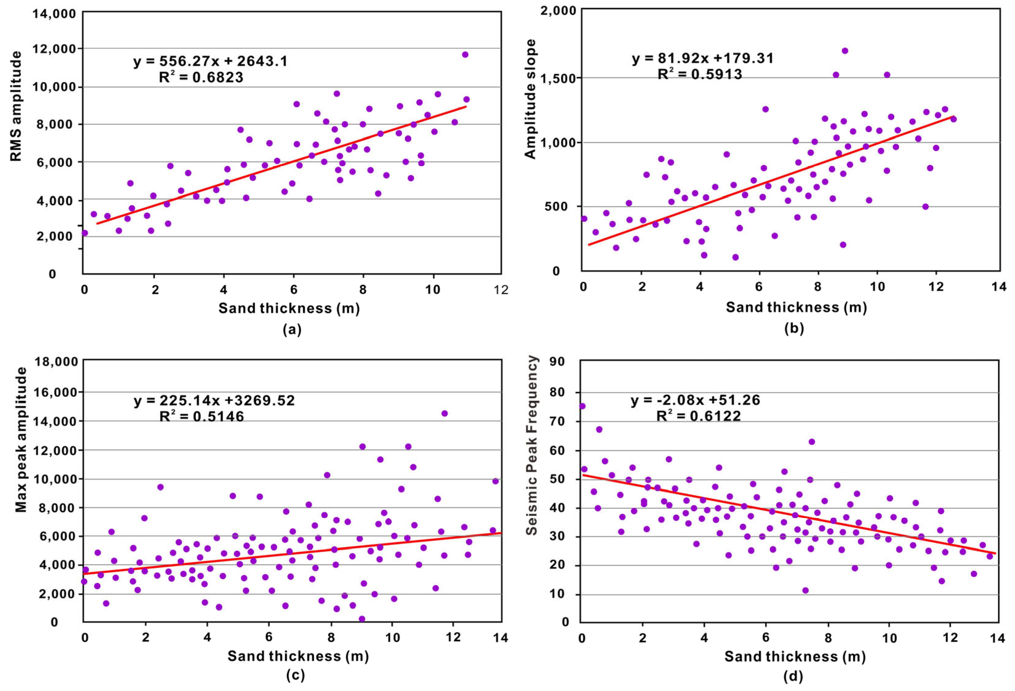
Seismic data are vital for predicting sandbodies and they are characterized by horizontal continuity and a wide coverage. Firstly, the paper extracted 12 seismic attributes that fall into the categories of amplitude, phase, and frequency. Then, correlation coefficients were calculated based on the seismic attributes surrounding the well and sand thickness explained by the log curve. Lastly, the paper selected four optimized seismic attributes sensitive to the sandbody development in the research area based on the values of correlation coefficients, including the RMS amplitude, MPA (maximum peak amplitude), Ampslp (amplitude slope), and SPF (seismic peak frequency). According to relevant findings, positive correlations exist between the RMSAmp, MPA, Ampslp, and sandbody thickness, while negative correlations exist between the SPF and sandbody thickness (Figure 7).

The RMS Amplitude has a minimum value in the mud-rock area. As the sandbody thickness increases, the attribute values grow, and the correlation coefficient is 0.68, suggesting high correlations (Figure 7a). The SPF and MPA are also positively correlated with the sandbody thickness, with the correlation coefficients of 0.59 and 0.56, respectively (Figure 7b,c). Their characteristics are basically consistent with that of the RMS amplitude while the positive correlations are less than the RMS amplitude. The SPF is negatively correlated with the sandbody thickness, with a correlation coefficient of 0.61 (Figure 7d). Other seismic attributes are excluded because their correlation coefficients with sandbody thickness are small.

3.2.2. Optimize Seismic Attributes

In the research area, four seismic attributes were selected based on the correlation coefficients, including RMSAmp, MPA, Ampslp, and SPF. Then, these attributes were processed and analyzed with the PCA method proposed in Chapter 2.2. Firstly, four optimized seismic attributes underwent standardized treatment to meet the distribution with a mean value of 0 and a variance of 1. Next, the weight coefficient of each standardized seismic attribute was determined according to Formula (1), and the calculation results were listed in

Table 1. Computed weights of four selected seismic attributes.

Seismic Attribute	RMS Amplitude	Maximum Peak Amplitude	Amplitude Slope	Seismic Peak Frequency
Weight (ωi)	2.00	1.75	1.54	1.21

.

The weight coefficient of RMSAmp and MPA was 2 and 1.75. RMSAmp and MPA are the most sensitive to sand bodies and had the largest weight coefficients. The AMPslp and seismic peak frequency are less sensitive towards sand bodies and had smaller weight coefficients, including 1.54 and 1.21. Next, each standardized seismic attribute timed its weight coefficient to work out the weighted attribute data. After that, the covariance matrix of the weight attributes mentioned above was calculated. Then, their characteristic vectors and characteristic values were obtained to work out four independent principal components with the PCA method. Each principal component is the linear combination of four weighted attributes and can be expressed as follows:

F₁ = 0.71X₁ + 0.51X₂ + 0.46X₃ − 0.58X₄
F₂ = 0.42X₁ + 0.69X₂ − 0.21X₃ − 0.35X₄
F₃ = 0.46X₁ + 0.28X₂ + 0.67X₃ − 0.24X₄
F₄ = −0.21X₁ + 0.41X₂ + 0.72X₃ + 0.65X₄

(3)

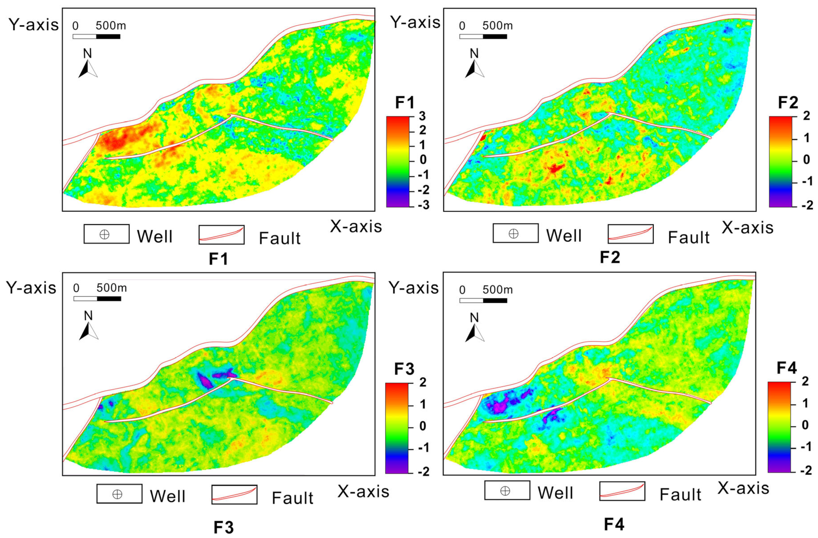
where F₁, F₂, F₃, and F₄ are the values of four principal components, X₁, X₂, X₃, and X₄, respectively, stand for RMSAmp, MPA, Ampslp, and SPF. Then the spatial distribution of four principal components was worked out based on four weighted seismic attributes with the formula above (Figure 8).

To optimize the principal components, the contribution rate and accumulative contribution rate of each principal component and correlation coefficient of the on-well sandbody development probabilities were calculated (

Table 2. Correlation coefficients of four principal components and the sand thickness, energy content, and cumulative energy content.

Principal Component	Correlation Coefficient	Energy Content (%)	Cumulative Energy Content (%)
F1	0.83	70.21	70.21
F3	0.51	9.25	79.46
F2	0.36	13.16	92.62
F4	0.14	7.38	100

).

The on-well sandbody development probability is equal to the ratio of the explained sandbody thickness and stratum thickness in the target stratum. The correlation coefficient between the first principal component and sandbody thickness was 0.83. The correlation coefficient between the third principal component and sandbody thickness was 0.52. Both correlations were significantly higher than those of other principal components. Meanwhile, the accumulative contribution rate of the first and third principal components exceeded 75%, including a majority of information concerning four seismic attributes. The second principal component had a higher contribution rate than the third principal component. However, the correlation coefficient between the second principal component and the sandbody thickness was smaller than that between the third principal component and the sandbody thickness. Thus, the second principal coefficient was excluded. Eventually, the paper selected the first and third principal components for predicting sandbodies.

3.2.3. Construct Elementary Conditional Probability Volumes

After determining the first and third principal components as research objects for the sandbody prediction, the paper demarcated the correlations between the first principal component and sandbody thickness and that of the third principal component to work out the basic conditional probability.

Firstly, the paper resampled the well along the trajectories of four seismic attributes, including RMSAmp, MPA, Ampslp, and SPF, to draw the seismic attribute curve. Then, the seismic attribute curve underwent standardized treatment to calculate weighted coefficients. Eventually, the first principal component curve and the third principal component curve were calculated based on Formula (3) [34].

After obtaining the logging curves of the first and third principal components, the paper divided the first and third principal components into several rows at a fixed interval and calculated the sandstone development probability corresponding to the principal component interval in each line (Histogram in Figure 9). The smooth curve (red line in Figure 9) was predicted based on statistical histograms, and the selected principal component was converted into the reservoir development’s elementary conditional probability. Under constraints of the smooth curve, the paper obtained the reservoir development probability under the conditional constraints of a single principal component.

3.3. Fusion of Elementary Conditional Probability and Modeling

In this section, the PR model was employed to combine two elementary conditional probability volumes in Section 3.2 and constructed a joint reservoir development probability. Then, the reservoir geostatistical modeling was carried out by combining the joint probability with the training images, including the 3D structure and stratum model, the facies model, the property model, and the dynamic numerical simulation model.

3.3.1. Obtain the Joint Probability with PR Model

This section aims to combine the elementary conditional probability volumes of the first and third principal components obtained in the previous section with the PR model, and to work out the joint reservoir development probability volume in the target stratum. Given the independence between the principal components, the PR model was employed to calculate the joint reservoir development probability [35]. Its calculation formula is listed as follows:

$${\mathrm{P}(\mathrm{k}}_{\mathrm{s}}{|\mathrm{F}}_1{,\mathrm{F}}_3)=\frac{\frac{{1-\mathrm{P}(\mathrm{k}}_{\mathrm{s}})}{{\mathrm{P}(\mathrm{k}}_{\mathrm{s}})}}{\frac{{1-\mathrm{P}(\mathrm{k}}_{\mathrm{s}})}{{\mathrm{P}(\mathrm{k}}_{\mathrm{s}})}+\frac{{1-\mathrm{P}(\mathrm{k}}_{\mathrm{f}}{|\mathrm{F}}_1)}{{\mathrm{P}(\mathrm{k}}_{\mathrm{f}}{|\mathrm{F}}_1)}\cdot \frac{{1-\mathrm{P}(\mathrm{k}}_{\mathrm{f}}{|\mathrm{F}}_3)}{{\mathrm{P}(\mathrm{k}}_{\mathrm{f}}{|\mathrm{F}}_3)}}$$

(4)

where Formula (4) is the specific manifestation of the PR model’s computing method (Formula (3)) in the research area; P (k_s|F₁, F₃) is the joint reservoir development probability volume under the common constraints of the first and third principal components; P (k_s) is the development probability of reservoir sandbodies in the research area and equals 0.65 in this case; P (k_s|F₁) and P (k_s|F₃) are the conditional probabilities of reservoir development under constraints of the first and third principal components.

Figure 10 presents the joint reservoir development probability of the target stratum in the research area. As is shown by the figure, the target stratum of the research area includes three stripped high-value areas of sandbody development probabilities with north–south striped distributions. These areas are partitioned by two low-value probability stripes. This characteristic strongly matches the seismic profile. Moreover, the sandstone development probability of every stripe decreases from the south to the north, which is consistent with the geological understanding that previous sediments originated from the Chenning Uplift in the south. Meanwhile, five new wells in the research area were not involved in the sandbody prediction, and the on-well reservoir development probabilities of Well 1, Well 4, and Well 5 were, respectively, 0.84, 0.87, and 0.81. The predicted joint reservoir development probability volume that corresponds to these three wells was greater than 0.8, and the reservoir development probability of Well 2 and Well 3 was 0.65 and 0.52, respectively. The predicted reservoir development probability corresponding to Well 2 was 0.69 and had a small error. The predicted reservoir development probability corresponding to Well 3 was 0.61 and had a high relative error. In conclusion, the reservoir development probabilities of five wells not involved in the PR model’s calculation were highly consistent with the predicted probability values, which proves the accuracy of the joint reservoir development probability.

3.3.2. 3D Structure and Stratigraphical Model

Firstly, a fault model was built based on eight pieces of fault interpretation data provided by oilfield corporations. Next, the on-well stratified data of twenty wells were regarded as hard data, and 3D structure models were built based on taking seismic interpretation data as inter-well trend surfaces. The model’s top-surface structure was high in the north and low in the south. The top surface surrounding the fault was −1320 m deep in the north and −1420 m in the south (Figure 11). The model’s length, width, and height were approximately 2500 m, 4000 m, and 40 m. The grid’s length, width, and height were 10 m, 10 m, and 1 m. The model consisted of 4,000,000 grids in total (250 × 400 × 40).

3.3.3. Facies Model and Property Model

The facies model was built with multi-point geostatistics based on the 3D structural model. Next, the models were built for porosity, permeability, and oil saturation with the Sequential Gauss Stimulation method.

The multi-point geostatistics of Petrel software was employed to construct the facies model. This method focuses on expressing correlations between multiple points by screening training images to reappear the target’s distribution characteristics effectively. Specifically, roughened wellbore facies interpretation data were collected as hard data, and the reservoir development’s joint probability volume was taken as constraint data. Then, this paper built a facies model for the research area by screening the deposit training images collected in Section 3.2. The porosity model was built in the following procedures: first, the on-well porosity curves of 20 wells were roughened and collected as hard data. Next, a variance analysis of the roughened logging curve data was carried out to determine the major and minor ranges’ directions and sizes in the modeling process. Figure 12 presents the major and minor ranges’ directions of the porosity model in the research area, as well as the experimental variance and fitting variance in two directions. The directions of the major and minor ranges are, respectively, 12.5° and 102.5°, and the ranges are 1396 m and 648 m, respectively. Lastly, the Sequential Gauss Simulation method of the Petrel software was employed to build a porosity spatial distribution model under the facies model’s constraints. Meanwhile, a model was built for the permeability and oil saturation through the Sequential Gauss Simulation method. The slight difference was that the facies model and porosity model were common constraint conditions for permeability modeling, while the oil saturation model was modified by the oil–water interface.

Given that random simulation is uncertain, the simulation was carried out 50 times for the facies model, the porosity model, the permeability model, and the oil saturation model. Next, these models were evaluated based on five unmodelled wells’ data to select the model with the highest matching degree. Figure 13 shows the selected facies model, the porosity model, the permeability model, and the oil saturation model.

3.3.4. Numerical Simulation of Oil Deposits

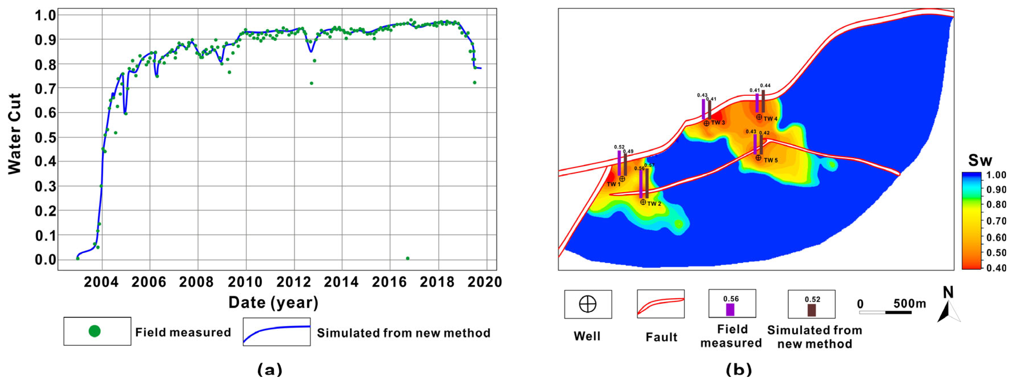
The numerical simulation of the oil reservoir was not the priority of this study. Instead, the paper focused on proving the accuracy of the built models by comparing the predicted water content and actual water content of five verification wells through numerical simulation. Firstly, a numerical simulation for the oil reservoir was carried out for the built models. The comparison showed that the research area’s overall water content had a high fitting, indicating that the built oil reservoir model has high accuracy (Figure 14a). Secondly,

Table 3. Statistical table of water cut change of 5 verification wells in the initial 6 months.

Date(Sw)	1 February 2020	1 March 2020	1 April 2020	1 May 2020	1 June 2020	1 July 2020
Well
TW1	52.16%	54.24%	56.33%	59.21%	61.71%	65.27%
TW2	56.12%	59.32%	62.23%	66.14%	74.16%	77.10%
TW3	42.87%	47.13%	49.33%	55.42%	61.23%	70.12%
TW4	41.25%	43.18%	48.32%	55.16%	57.14%	60.37%
TW5	43.27%	49.16%	55.34%	61.42%	69.10%	76.46%

displays the changes in the water content of five verification wells from the previous six months. As is shown by Figure 14, the water content predicted by the model was highly consistent with the water content and production data of the verification wells, which further proves the accuracy of the constructed facies model and attribute models.

4. Discussion

4.1. Merits of New Deposit Prediction Method

The new reservoir prediction method proposed by this paper obtained the spatial distribution of fluvial reservoirs more clearly. By comparison, the proposed reservoir prediction method is more advantageous than the traditional probability fusion method and the simulation results of single seismic attributes. The RMS amplitude was most sensitive to sandbody development and was thus selected as the object for comparison. Then, the correlations between the seismic profile and plane were analyzed to prove that the proposed method identifies the river-channel sandbodies’ boundaries more effectively. Three river-channel belts could be identified from the seismic profile of the research area. Well 6 and Well 10 are located in two river-channel sandbodies, and the actual production data proved that they were unconnected. The probability plane graph obtained from the RMS amplitude could hardly differentiate between the boundaries of river-channel sandbodies. The probability plane graph obtained by the traditional probability fusion method reflected the sandbody boundaries more effectively than the RMS amplitude, yet it still fell short of the proposed method (Figure 15). The coefficient of correlations between the sandbody probability predicted by the traditional probability fusion method and the actual on-well sandbody’s development probability was 0.726, and the new method’s correlation coefficient was 0.832, proving that the new method’s prediction results were significantly better than those of the traditional probability fusion method.

Error δ₁ was introduced to compare the differences between the proposed new method and the traditional probability fusion method quantitively. The error was defined as the average difference between the predicted probability and the actual on-well probability, and its calculation formula is as follows:

$$\mathsf{\delta }1=\frac{{\sum }_{\mathrm{i}=1}^{\mathrm{n}}{|\mathrm{P}}_{\mathrm{i}}^{\prime }{-\mathrm{P}}_{\mathrm{i}}|}{\mathrm{n}}{,\mathrm{P}}_{\mathrm{i}}=\frac{{\mathrm{h}}_{\mathrm{si}}}{{\mathrm{h}}_{\mathrm{i}}}$$

(5)

Figure 16 presents the error between the sandbody development probability predicted by the two probability fusion methods under different numbers for the seismic attributes and the actual probability. Each seismic attribute was added in the descending order of its correlation coefficient with the sandbody development probability. When only one attribute was selected, two methods had consistent errors. As the number of seismic attributes increased, the new deposit prediction method’s error was significantly smaller than the traditional method, and the difference was widening. When four seismic attributes were selected, the new method reduced errors by 32%.

As more seismic attributes are added, the new method’s prediction error and the range of error variations shrinks. This can be explained by the following fact: with the PCA, each principal component remains independent, has no informational redundancy, and meets the PR model’s hypothetical conditions. Thus, increasing the number of seismic attributes lowers the prediction error. For another, each seismic attribute is given a weight based on the correlation coefficients in the PCA. The seismic attributes sensitive to sandbody development have a high contribution rate and are always selected first. As a result, the range of error variations shrinks as the number of seismic attributes increases. By comparison, the errors of traditional methods first decrease and then increase. There are no significant correlations between the range of error variations and the number of seismic attributes because the traditional methods fail to guarantee independence between the seismic attributes. When the number of seismic attributes increases from 1 to 2, the correlation coefficients between two seismic attributes and the sandbody are high. In addition, the error decreases because the effective information included by the second seismic attribute makes a greater contribution to the accuracy of the sandbody prediction than the loss resulting from informational redundancy between two pieces of seismic information. As the third type of seismic information is added, its contribution to the prediction accuracy equals the loss caused by the information redundancy. Thus, the prediction error does not change significantly. When the fourth type of seismic attribute is added, its sensitivity towards the sandbody is lowered, and its contribution rate is lower than the loss, which increases the prediction error. In conclusion, the new method can effectively increase the accuracy of predicting braided fluvial facies deposits.

4.2. Dynamic Verification

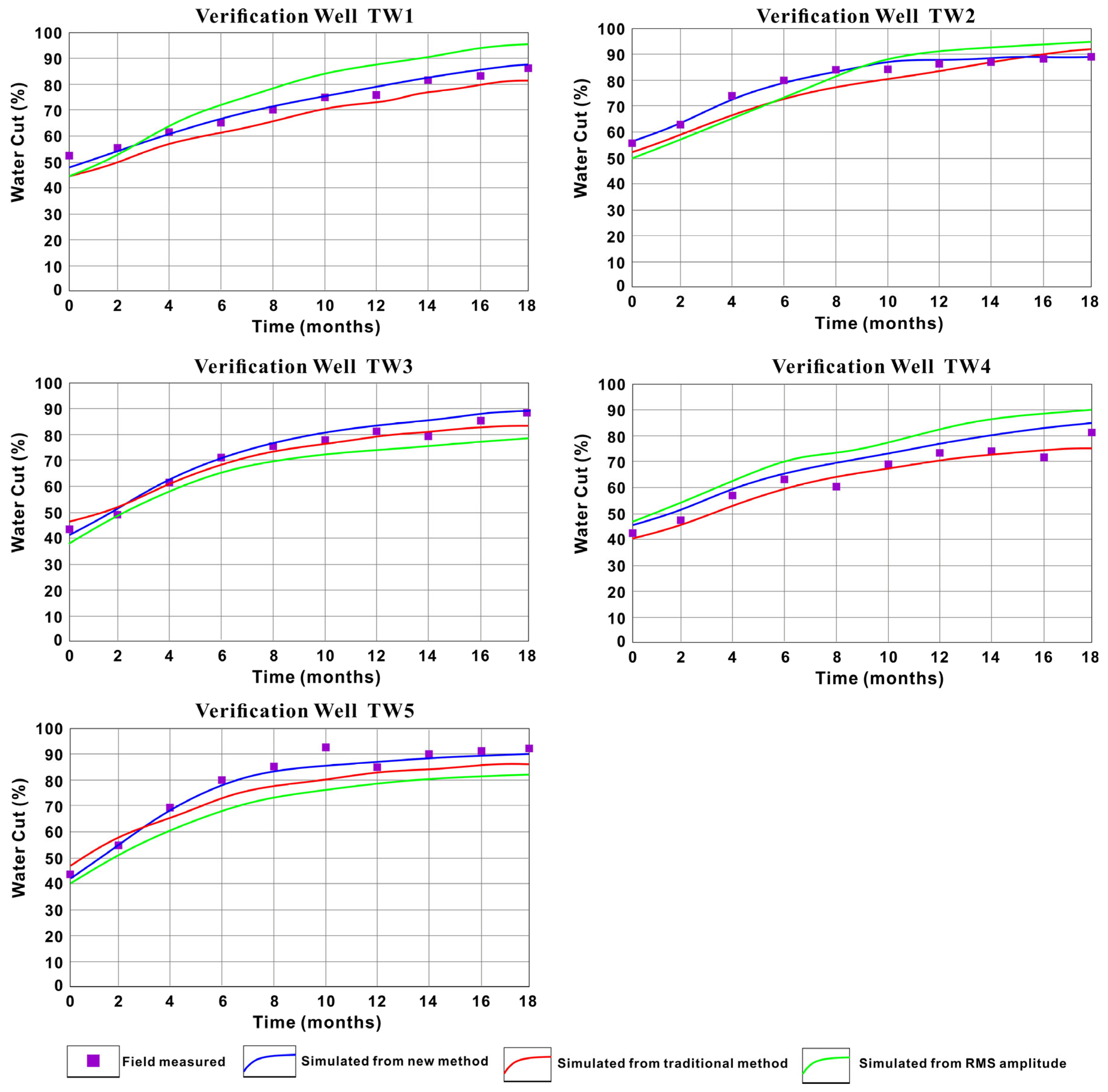
Firstly, models were constructed for the porosity, permeability, oil saturation, and other attributes of the target stratum in the research area. Next, the numerical simulation was carried out in the research area, and five wells uninvolved in the modeling were selected for verification. The errors between the actual on-well water content and predicted water content were evaluated to compare the accuracy of different methods. Figure 17 compares the actual water content of five horizontal wells in the research area and the water content calculated with the traditional probability fusion method, the improved probability fusion method, and the probability volume simulation of RMSAmp. In the simulation, consistent static and dynamic parameters were used, including identical training images, logging curves, fluid properties, and production pressure. As is shown by the figure, the water content predicted with the new method matches best with the actual on-well water content, followed by the water content predicted by the traditional probability fusion method. The water content predicted by the RMSAmp’s probability volume deviates most from the actual water content. To quantify the differences between different prediction methods, error δ₂ was introduced and defined as the average value of the difference between the predicted water content and actual water content. The calculation formula is listed as follows:

$$\mathsf{\delta }2=\frac{{\sum }_{\mathrm{i}=1}^{\mathrm{N}}{|\mathrm{W}}_{\mathrm{i}}^{\prime }{-\mathrm{W}}_{\mathrm{i}}|}{\mathrm{N}}$$

(6)

where W′_i is the predicted water content of the ith month; W_i is the actual water content measured at the oilfield in the ith month; and N is the number of data concerning the production well’s water content.

The errors for the water content calculated with different prediction methods (Figure 17) were compared. The average error of the water content predicted with the new method was 4.76%; the average error calculated by the traditional probability fusion method was 7.5%. The water content calculated by the RAMAmp’s probability volume was the lowest and had an error of 12%. Compared with the latter two methods, the new method proposed by this paper increases the prediction accuracy by 36.5% and 60.3%.

As is shown above, the reservoir prediction method proposed by this paper can effectively increase the prediction accuracy. To clarify that this proposed method is based on the contribution rate of training images from modern sedimentation and field paleo-outcrops, this paper designed two scenarios, including modeling with training images and modeling without training images. Then, a numeric simulation was carried out to compare and test the error between the actual water content and the predicted water content. The simulation results eventually proved the advantages of obtaining training images based on modern sedimentation and field paleo-outcrops. The proposed method essentially builds the modeling based on multi-point geostatistics with training images. In another scenario, training images were not involved in the modeling, and the improved probability composite was taken as the constraint condition, then the coordinated sequence instruction simulation of Petrel software was employed to build geological models and carry out the numerical simulation. Both methods employed consistent parameters in the attribute modeling and numeric simulation.

The error between the water content predicted by the reservoir prediction method based on the improved PR model with multi-point geostatistics and the actual water content was significantly smaller than the calculation error calculated by the PR model with two-point geostatistics (

Table 4. Errors of water cut simulated from reservoir models established by the methods with training images or not.

Errorw	TW1	TW2	TW3	TW4	TW5	Average
reservoir model established with training image	3.46%	3.72%	4.58%	6.43%	5.61%	4.76%
reservoir model established without training image	12.38%	11.53%	9.54%	9.16%	12.64%	11.05%

). The average error of the former method and the latter method was 4.76% and 11.05%. The reservoir prediction method based on the improved PR model and multi-point geostatistics increased the prediction accuracy by 56.92%.

At the same time, at present, the method proposed in this paper mainly depends on seismic data, and the application of the logging curve and thin section data is less flat, which is a problem to be improved in the next step.

5. Conclusions

Predicting the spatial distribution of braided fluvial facies reservoirs is a vital step in exploring and developing oil reservoirs. This paper proposes a reservoir prediction method based on the improved probability fusion model and combining it with the multi-point geostatistics. The error between the actual development probability data of on-well sandbodies and the predicted sandbody development probability was compared. It was proved that the new method increased the prediction accuracy by 32% relative to the traditional probability fusion method. Meanwhile, the model constructed with the new method matched with dynamic materials better. According to the matching relations between the actual water content and predicted water content of five verification wells, the new method lowered the prediction error by 60.3% and 36.5% relative to the method based on RMSAmp and the traditional probability fusion method. Meanwhile, the paper demonstrated procedures for predicting the spatial distribution of braided fluvial facies reservoirs and constructing spatial distribution models of reservoirs.