Numerical Analysis of Heat Transfer within a Rotary Multi-Vane Expander

Abstract

In this paper, the results of numerical investigations on heat transfer in a multi-vane expander (MVE) are reported. MVEs are very interesting for various technological applications because of their advantages (such as, for example, low gas flow capacity and a low expansion ratio). According to a literature study, the heat exchange mechanisms occurring in these machines have not yet undergone in-depth analysis. As a result, there have been very few experimental or modeling results connected to these unquestionably significant processes from both a scientific and practical perspective. Despite the fact that several analytical models have been developed for these phenomena, there is no numerical model dedicated to an MVE. This model was developed by the authors and presented in this paper together with modeling results. Numerical simulations were executed in the ANSYS CFX and focused on defining the expander heat transfer coefficients under various flow circumstances. The results showed inside heat transfer processes in MVEs and, moreover, it was discovered that, in the gap between the vane and the cylinder, there are changes in the fluid’s velocity profile.

1. Introduction

Multi-vane machines are positive displacement machines, the operation of which which are based on the rotational movement of the components. These machines are successfully applied as expanders, compressors, liquid pumps, and vacuum pumps in various technical applications. Multi-vane compressors are used in refrigeration, air conditioning, and pneumatic systems. Multi-vane pumps are primarily used in these applications in which the required flow output is low and moderate fluid pressure is needed. Multi-vane expanders (MVEs) are primarily applied as motors in these applications in which a risk of flammable gas explosion occurs, and thus the use of electric tools is limited. Such applications include driving pneumatic tools in mining or mixing machines in the chemical industry. Moreover, multi-vane motors are used in other applications, such as dentistry drills.

MVEs developed for modern domestic organic Rankine cycle (ORC) systems have recently attracted more attention for low or micro power from 1 to 3 kWe. This is mainly due to their simple construction, which has fewer moving parts, makes them easier to manufacture, and has lower production and acquisition costs than, for example, microturbines with equivalent power [1]. Additionally, they have a power range that makes them appropriate for these uses (the power of MVEs is in the range of several hundred watts to ca. 10 kW, while 10 kW is the maximum power of expanders currently produced [2]). In many scientific institutions across the world, since the 1970s, there have been studies on the application of MVEs in ORC systems. These studies were first conducted by NASA as part of research on their possible utilization in space applications. The results of these tests are presented in more detail in [3]. Badr et al. carried out a comprehensive experimental and theoretical analysis of MVEs at Cranfield University in the 1980s [4,5,6,7,8,9,10,11,12,13,14]. In addition to promising experimental results, numerous mathematical models useful for modeling the expander operation, including vane kinematics, friction, and forces in the machine, were presented. In the 1990s, research on the potential application of an MVE in the ORC system was carried out at Wrocaw University of Technology by Prof. E. Kalinowski and his team [15]. As a part of this research, Z. Gnutek defined a new function, i.e., Z(ϕ) application, which enabled easier modeling of the processes occurring in the expanders’ working chambers [16].

The test stands were developed as a part of the aforementioned study, experimental data was gathered, and several mathematical models explaining the operation of the machine were established. These models make it feasible to calculate the volume change of the working chamber calculations, as well as the forces’ variability and friction within the machine. However, the practical applicability of these models is limited as they are complex analytical models. They can be used to conduct detailed, but not entirely accurate, analyses of the machine operation. Currently, it is possible to provide much more accurate simulations of MVE operation and provide guidelines for their optimization using computer simulation tools, such as ANSYS, OpenFOAM, and other software. For instance, some cases were discussed in [17].

As this brief survey of the literature has shown, previous studies [4,5,6,7,8,9,10,11,12,13,14,15,16] have mainly focused on analytic or experimental evaluation of expander operation (i.e., estimation of thermodynamic parameters of the working fluid inside the MVE working chamber, expander power and efficiency, etc.), while the heat exchange mechanisms occurring in these machines have not been thoroughly studied to date. For this reason, heat transfer models are rare in the literature, and there have been no numerical models reported. Only few experimental and modeling findings pertaining to these processes are available (and are detailed in more depth later in this article). Although some analytical models for these phenomena have been developed, a thorough numerical model analysis is required. From a scientific and practical perspective, heat exchange processes within and outside the machine have considerable influence on its performance and efficiency. These phenomena are incredibly challenging because several thermodynamic and hydrodynamic processes, including the circulation of the working fluid within the chamber, the impact of the flow on the surface of the machine parts, or the leakage between adjacent working chambers, simultaneously occur in the MVE working chamber described in Section 2 for the MVE operation (through the gaps between the top of the vanes and the cylinder, and through other leaks). The occurrence of the boundary layer being scraped by a vane has a substantial impact on the process of heat transfer in a multi-vane machine. As a result, the fluid velocity profile in the gap between the vane and the cylinder is subsequently disturbed.

The authors, encouraged by the complexity of these problems, decided to model the heat exchange phenomenon in an MVE using an ANSYS software based on the experience acquired in previous research on the application of MVEs in ORC systems. To the knowledge of the authors, this is the first numerical attempt to model heat transfer in MVE, and this is the state of the art feature of this investigation. The structure of the article is as follows. Firstly, the description and principle of operation of an MVE are introduced. Then, the heat exchange processes occurring in an MVE are described. In the next part of the article, we present the numerical model used in the analysis, the results of the numerical modeling, and the resulting conclusions. The numerical model used in this article was developed on the basis of the geometry of the real MVE, which was used by the authors in previous studies and was described in detail in [18]. The pressure and temperature of the working fluid, the expander shaft’s rotational speed, and other operational parameters of the simulated expander correspond to those of the actual expander utilized in the studies.

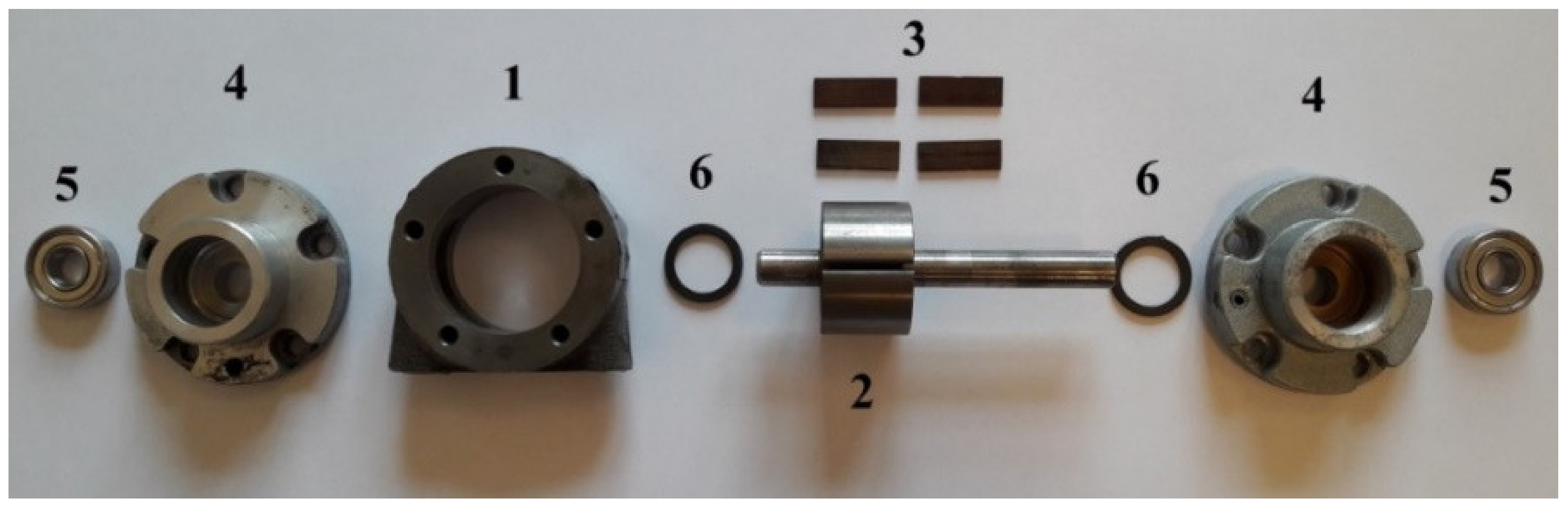
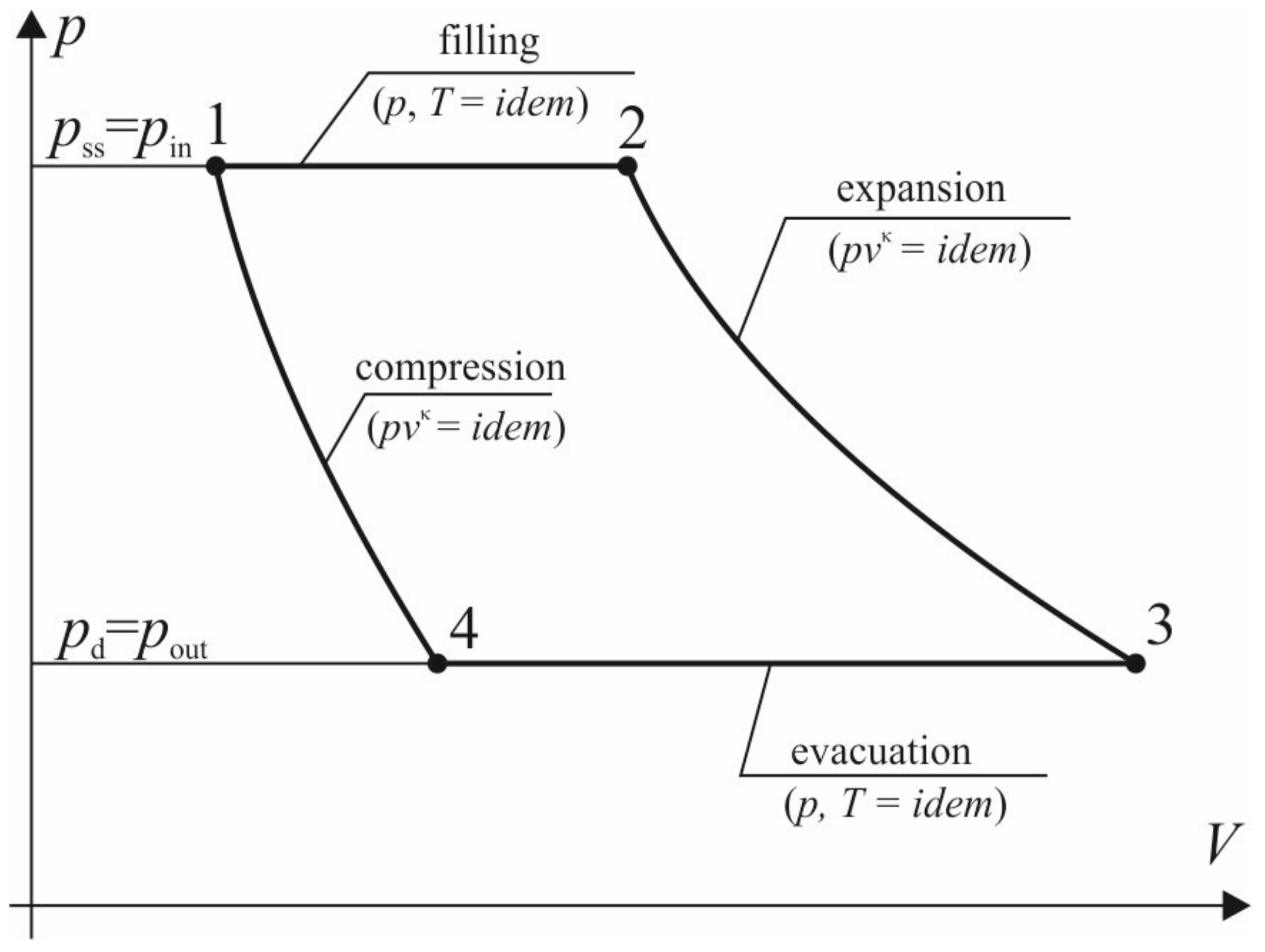
2. Description of the Multi-Vane Expander Assembly and Principle of Operation

The assembly of the MVE can be clearly described on the basis of Figure 1 and Figure 2. In its basic design, an MVE is composed of a cylinder (1), rotor (2), vanes (3), side covers (4), bearings that support the shaft of the rotor (5), and vane guide rings (6). It should be clarified here that the vane guiding ways are different and depend on the expander design. Instead of vane guide rings, some MVEs are equipped with vane springs. The vane guiding by means of centrifugal force is also applied in some of the MVEs.

The rotor (2) of the radius r is eccentrically placed in the cylinder (1) of the radius R (where e is eccentricity). The vanes (3) are placed in the guiding slots milled in the rotor (see item 4 in Figure 2) and pressed against the surface of the cylinder (1) by means of guiding rings (6). During rotational movement of the rotor with angular velocity ω, the vanes move forward and backward in the slots. The cylinder is closed with side covers (4), where the bearings are mounted (5). Depending on the expander design, rolling or sliding bearings are applied.

The eccentric arrangement of the cylinder and the rotor results in working chambers being formed between the surfaces of the cylinder, the rotor, and two nearby vanes. Throughout the rotational movement of the rotor, the working chamber’s volume is continually changing. The working fluid is fed under high pressure to the expander inlet port through an inlet connection which is usually located on the bottom or side of the cylinder. The gas pressure exerted on the vane puts the rotor in a clockwise rotational movement. During the rotational motion of the rotor, the volume of the working chamber rises. Therefore, the working fluid that is enclosed in the chamber expands. The expansion is accompanied by a gas pressure and a temperature drop. After a certain part of the rotor revolution, the working chamber is opened to the discharge region and the working fluid is evacuated from the chamber. The edges of the inlet and outlet ports of the MVE act as a camshaft in piston machines, therefore, they are referred to as control edges. Their proper arrangement is important and influences the operating conditions of the machine. This issue is discussed in more detail in [18]. The MVE operating cycle consists of successive processes of filling, expansion, evacuation, and compression of residual working fluid. For an ideal expander cycle, one assumes that the filling and evacuation processes are isobaric and that the expansion of the working fluid and compression of the residual working fluid occur according to adiabatic processes. This ideal expander cycle is usually used as a refence cycle, thanks to which it is possible to assess the energy losses and efficiency of the real MVE. This cycle is depicted in Figure 3 in a p-V diagram.

The cycle of the real MVE differs from the ideal one due to the energy losses occurring in the real machine. These energy losses are associated with flow throttling during filling and evacuation of the working fluid, internal and external leakages, friction, and heat transfer. Therefore, in the real cycle, the residual fluid expansion and compression processes are usually treated as polytropic.

During the expansion of the working fluid in the expander, the gas pressure decreases, which leads to a significant decrease in its temperature. This phenomenon also affects the nature of the heat transfer processes in the expander. It should be noted here that the effect of compressing the residual working fluid on the real expander cycle is negligible due to the very small clearance volume, which is practically limited to the volume of the machine inlet port. The indicator diagram of the real MVE was recorded during the experiments, and the results are presented in [5]. This diagram is depicted in Figure 4. The diagram is valid for the eight-vane expander that works with R113. During this experiment, the rotational speed of the expander (n) was 2820 rpm and the working fluid temperature at the inlet of the expander (t_in) was equal to 107 °C. The pressure of the working fluid at the inlet and outlet of the expander (p_in) was equal to 0.51 MPa and 0.14 MPa, respectively.

The following undoubted advantages of MVEs can be listed:

• simple design,
• ease of installation and service,
• a small number of moving parts,
• the ability to work with a small flow of working fluid,
• large pressure drops that are possible to obtain in one stage,
• optimal expansion ratio in the range of 2–4,
• low weight and dimensions in relation to the power output,
• power range suitable for use in domestic micro power plants (the maximum power of currently manufactured expanders is about 10 kW),
• low rotational speed enabling the direct transmission of torque, to the generator as an example,
• lack of valves,
• the possibility of implementing oil-free and hermetic expanders,
• the possibility of using different working fluids, and
• insensitivity to wet gas expansion.

3. Heat Exchange Processes Occurring in a Multi-Vane Expander

The working chambers of an MVE are concurrently experiencing a variety of physical phenomena. The most significant phenomena are the following:

• flow of working fluid through the working chambers,
• circulation of working fluid within working chambers and how its impact on machine parts,
• external and internal leakages of the working fluid,
• friction,
• temperature of the working fluid changes during processes (depending on the character of the machine operation, i.e., temperature drop when using cooled compressors and expanders to expand hot gasses, or temperature rise when using cold gas expanders, which expansion causes a further significant drop in gas temperature which can lead to, for example, the formation of hydrates [19]), and
• cooling (or heating) fluid to cool (or heat) the machine.

The conditions of heat transfer in the machine are affected by these operations. In consideration of the phenomena just described, the machine’s internal heat transfer rates can be given as follows:

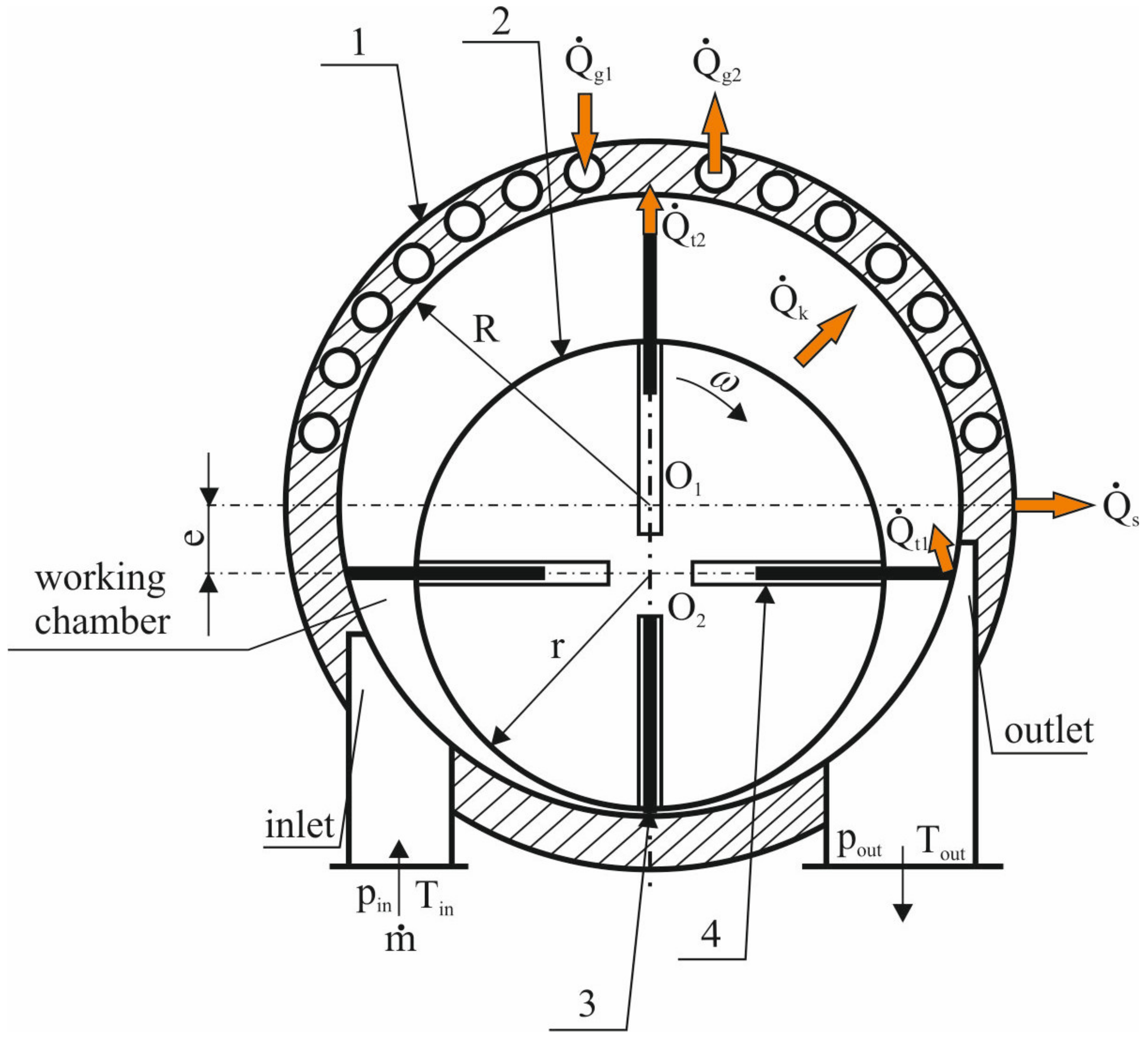
• $\dot{Q}$_g1 is the heat transfer rate at which heat from heated fluid is transferred to the working fluid,
• $\dot{Q}$_g2 is the heat transfer rate at which is taken from the working fluid by the cooling fluid,
• $\dot{Q}$_s is the heat transfer rate at which is dissipated from the surface of the machine to the surroundings,
• $\dot{Q}$_t = $\dot{Q}$_t1 + $\dot{Q}$_t2 describes the heat transfer rate at which is produced as the result of friction,
• $\dot{Q}$_t1 is the heat transfer rate that is generated as a result of friction and transferred to gas;
• $\dot{Q}$_t2 is the heat transfer rate that is generated as a result of friction and transferred to the parts of the machines, and
• $\dot{Q}$_k is the heat transfer rate at which is transferred by convection from (or taken by) gas to the walls of the working chamber.

Figure 5 provides a detailed description of the heat transfer processes that take place in the MVE.

Equation (1) represents the heat transfer rate from (or absorbed by) the machine surface to (from) the environment.

$${\dot{Q}}_s=h_s\left(T_c-T_{air}\right)A$$

(1)

where h_s, A, T_c, and T_air describe surface film conductance from the (to) machine surface to (from) the environment, the heat exchange surface (outer surface of the machine), the temperature of the machine surface, and the temperature of the surroundings, respectively. Equation (2) is used to define the heat transfer rate from the heating fluid to the gas.

$${\dot{Q}}_{g1}={\dot{m}}_1{c}_{p1}\left(T_{1in}-T_{1out}\right)$$

(2)

where: T_1in, T_1out, $\dot{m}$₁, and c_p1 describe the temperature of the heating fluid at the inlet to the machine, the temperature of the heating fluid at the outlet of the machine, the mass flow of the heating fluid, and the heat capacity of the heating fluid, respectively. Equation (3) may be used to calculate the rate at which heat is transferred from the gas to the cooling fluid.

$${\dot{Q}}_{g2}={\dot{m}}_2{c}_{p2}\left(T_{2in}-T_{2out}\right)$$

(3)

where: T_2in, T_2out, $\dot{m}$₂, and c_p2 describe the temperature of the cooling fluid at the inlet to the machine, the temperature of the heating fluid at the outlet of the machine, the mass flow of the cooling fluid, and the heat capacity of the cooling fluid, respectively. Equation (4) describes the heat of friction (expressed in J), as shown in [21],

$$Q_{fe}=\left(1-K_{fe}\right)L_{fe}$$

(4)

where Q_fe, L_fe, and K_fe represent friction heat emitted during the operation of the moving element, the work needed to overcome friction, and the total input of non-thermal components of friction in energy expenditure, respectively. In this case, K_fe = 0.04–0.08 [22]. Equation (5) may be used to express the output of the friction heat source (in W/m²) given the contact surface of the rubbing elements [22],

$${\dot{q}}_{fe}=\left(1-K_{fe}\right)N_{fe}\frac{1}{A_s}$$

(5)

where N_fe and A_s describe the power consumed to overcome the friction of the element and the contact surface of the rubbing elements, respectively.

The phenomena of heat exchange in a rotating working chamber are the most interesting heat exchange phenomena in a multi-vane machine from a scientific perspective. Heat transfer mechanisms in MVE are different than in the case of other volumetric machines and energy devices. The rotating rotor and vanes significantly influence this mechanism. For example, vanes are scraping the boundary layer at the cylinder wall. This phenomenon is similar to the processes that occur, for instance, in scrapped heat exchangers. Therefore, a description of this process has to be included in mathematical and numerical models. According to [21], the relationships between the convective heat transfer applied to the flow around flat surfaces can be used to calculate the heat transfer coefficient h under the assumption that this surface has a length of l equal to the circumference of the working chamber. The speed of the flowing working fluid w is then determined using Equation (6),

$$w=2\omega r$$

(6)

where r represents the radius of a circle, the perimeter of which is the same as the perimeter of the cross section of the working chamber; furthermore, ω describes the angular velocity of the working chamber. With the aforementioned presumptions in mind, the following relation for the Nusselt number Nu for the laminar boundary layer (for Re_l < 10⁵) can be used, which is described in Equation (7). Moreover, Equation (8) can be used for the turbulent boundary layer,

$$Nu=0.66{\mathrm{Re}}_l^{0.5}{\mathrm{Pr}}_p^{0.33}{\epsilon }_r$$

(7)

$$Nu=0.037{\mathrm{Re}}_l^{0.8}{\mathrm{Pr}}_p^{0.43}{\left(\frac{{\mathrm{Pr}}_p}{{\mathrm{Pr}}_s}\right)}^{0.25}$$

(8)

where ${\mathrm{Re}}_l=\frac{\omega l^2}{\nu }$ is the Reynolds number for the flat surface (where ν is a kinematic viscosity and l is the length corresponding to the circumference of the working chamber), ${\mathrm{Pr}}_p=\frac{\eta c_p}{k}$ is the Prandtl number (p stands for the fluid temperature), Pr_s is the Prandtl number (s stands for the wall temperature), where η is dynamic viscosity, cp is specific heat capacity at constant pressure, and k is thermal conductivity of the working fluid. ε_r is a factor depending on changes in the physical properties of the working fluid with a change in temperature.

The average value of the heat transfer coefficient from the working chamber’s walls into the gas may be determined using Equation (9).

$$h_s=Nu\frac{k}{l}$$

(9)

The occurrence of a vane scraping the boundary layer has a significant effect on heat transfer processes in multi-vane machines. Equation (10) may be used to obtain the Nusselt number under this condition [21].

$$N{u}_{\delta }=0.0228{\mathrm{Re}}_{\delta }^{0.75}{\mathrm{Pr}}^{0.33}, \mathrm{where} N{u}_{\delta }=\frac{h\delta }{k_g}$$

(10)

In this case, the Reynolds number can be calculated from Equation (11),

$${\mathrm{Re}}_{\delta }=\frac{w_l\delta {\rho }_g}{\eta }$$

(11)

where w_l and δ describe the linear velocity of the vane face moving along the cylinder and the thickness of the boundary layer for the free flow of the surface considered, respectively.

Scraper heat exchangers are one example of a device in which the phenomenon of the boundary layer being scraped by moveable parts disrupts fluid flow. One of the authors previously conducted a study on similar topics and presented the results in [23,24,25]. Based on the analyses conducted, the author developed the equation in Equation (12), which binds the Nusselt, Reynolds, and Prandtl values for these heat exchange conditions (m index denotes mixing).

$$Nu=1.765{\mathrm{Re}}_m^{0.496}{\mathrm{Pr}}^{0.33}$$

(12)

The authors chose to include this association in the current study due to the similarity of the observed events. There are no known Nusselt correlations in the literature that are applicable only to multi-vane devices. This makes it impossible to directly compare the proposed model to models from the literature. Nevertheless, the authors chose the machine with the most comparable heat transfer circumstances to make some comparison. This machine is a scraped surface heat exchanger [23,24] in which scraping vanes constantly scrape the inner wall of the cylinder to intensify the rate of heat transfer. Similar circumstances apply to MVEs, with the exception that the vanes’ function in these devices is to divide neighboring working chambers rather than to improve heat transmission.

Table 1. Several models of heat transfer [20].

Model	Correlation for the Nu	Notes	Refs.
ZG	$Nu=0.037{\mathrm{Re}}_l^{0.8}{\mathrm{Pr}}_p^{0.43}{\left(\frac{{\mathrm{Pr}}_p}{{\mathrm{Pr}}_s}\right)}^{0.25}$	Rel > 105	[21]
K-K	$Nu=\frac{hD}{k}=\frac{\cancel{k}}{\delta }\frac{D}{\cancel{k}}=\frac{D}{\delta }$	-	[26]
K-L-H	$Nu=\frac{2}{\sqrt{\pi }}\sqrt{n{\mathrm{Re}}_D\mathrm{Pr}}$	${\mathrm{Re}}_D=\frac{n{D}^2\rho }{\eta }$	[27,28,29]
P-B	$Nu=\frac{1}{\frac{\delta }{D}+\frac{1}{\sqrt{\frac{8}{\pi }{\mathrm{Re}}_D\mathrm{Pr}}}}$	-	[30]
P-Bexp	$Nu=1.123{\mathrm{Re}}_m^{0.78}{\mathrm{Pr}}^{0.33}{\left(\frac{{\eta }_b}{{\eta }_w}\right)}^{0.18}$	Rer > 400 ethylene, glycol	[31]
B-P	$Nu=1.765{\mathrm{Re}}_m^{0.496}{\mathrm{Pr}}^{0.33}$	Pr < 1	[24]
E	$Nu=0.11{\mathrm{Pr}}^{0.35}{\left(0.5{\mathrm{Re}}_w^2\right)}^{0.35}$	-	[21]

summarizes the equations employed in the simulations, which were used by the authors in previous studies [20]. D denotes the diameter of the cylinder and n is the rotational speed. Indices b and w refer to the bulk and wall conditions, respectively.

4. Numerical Modeling

4.1. Physical Model

The physical model, which was prepared based on the geometrical dimensions of the real rotary MVE (illustrated in Figure 1), is shown in Figure 6. The expander consists of a stationary cylinder with an inner diameter of 37.5 mm and a rotating rotor with an outer diameter of 34 mm. In the inner cylinder, four grooves are milled in which four vanes can move. Furthermore, the inner cylinder is positioned with an eccentricity of 1.75 mm to allow a change in the height of the vanes, and thus, the volume of the working chamber. Compressed air enters the expander through the inlet port, which has an inner diameter of 8.5 mm, and outflows through the outlet port, which has an inner diameter of 8.5 mm. The expander is placed in calm air at 15 °C. To simplify the calculations, the walls of the expander housing are not included in the model. With the movement of the rotor, the vanes move as well and slide on the inner surface of the cylinder. However, in real constructions of rotary vane expanders, the tips of the vanes do not perfectly contact the cylinder surface and small gaps exist, which are the reason for leakages between consecutive working chambers. Therefore, in the model, a small gap of 40 m in width of 40 µm between the tip of the vane and the inner surface is maintained.

4.2. Governing Equations

The flow in the expander is three-dimensional, transient, and turbulent. To obtain the thermal flow characteristics within the expander, an improved model presented in [18] was developed. The following partial differential equations were solved using ANSYS CFX software [32], where the equations of continuity, momentum, and energy are described in Equations (13), (14), and (15), respectively.

$$\frac{\partial \rho }{\partial t}+\nabla \cdot \left(\rho U\right)=0$$

(13)

$$\frac{\partial \rho U}{\partial \tau }+\nabla \cdot \left(\rho UU\right)=-\nabla p+\nabla \cdot \left[\mu \left(\nabla U+\nabla U^T\right)\right]$$

(14)

$$\frac{\partial \left(\rho h\right)}{\partial t}+\nabla \cdot \left(\rho Uh\right)=\nabla \cdot \left(k\nabla T\right)+\mathsf{\Phi }$$

(15)

where Φ is the dissipation function that takes into account the energy dissipation into heat within the working fluid. It was necessary to include this term because high velocities inside the expander (Ma > 0.3) appeared. Additionally, it turned out that including this term relaxes the temperature field and reduces high peaks in the Nusselt number distribution.

During the calculations, the shapes of the working chambers constantly changed. Therefore, at the beginning of each timestep, new positions of the boundary mesh nodes were calculated on the basis of geometrical changes in the expander boundaries. These equations were implemented in the CEL language [33]. Then, the distribution of internal nodes was obtained by solving the diffusion equation, which is expressed in Equation (16).

$$\nabla \cdot \left({\mathsf{\Gamma }}_{disp}\nabla \delta \right)=0$$

(16)

where δ is the displacement relative to the previous mesh locations and Γ is the mesh stiffness. This method is already implemented in the CFX software and is called the displacement diffusion model [26]. The advantage of this model is that it preserves the relative distribution of the nodes of the initial mesh.

To take into account the phenomenon of turbulence in the expander model, the SST turbulence model was utilized [32].

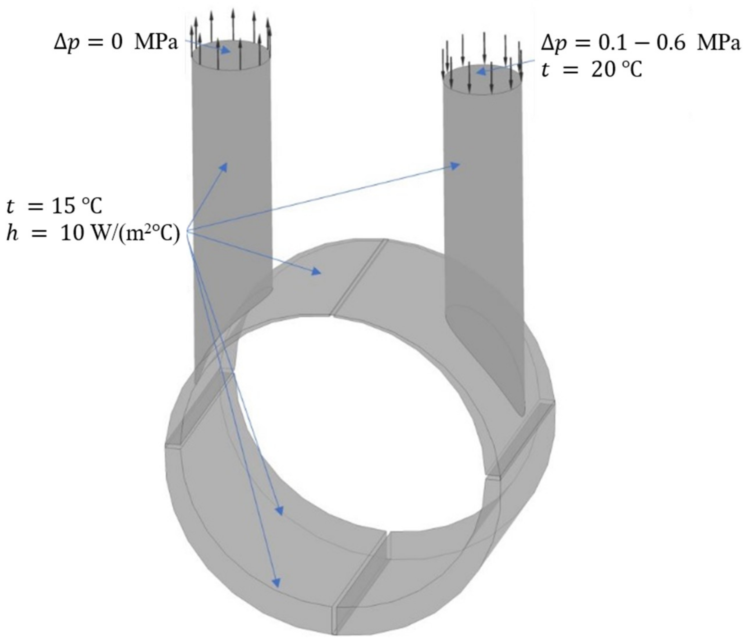
4.3. Boundary Conditions and Simulation Settings

In the initial stage of research, several tests were performed. It was found that a periodic steady state is achieved after one full revolution of the expander vanes. For this reason, it was decided to perform calculations for the time of three full revolutions to minimize computational time. Moreover, to be able to perform a numerical simulation without floating-point conditions, the timestep had to be lowered to the value that corresponds to the time interval needed to rotate the expander vanes by 0.1°.

The walls of the expander were not included in the model. They were modeled using boundary conditions. On the outer, inner, and side surfaces of the expander, the boundary condition of the third type was used with an ambient temperature of 15 °C and a heat transfer coefficient of 10 W/(m²·K). On the other hand, the surfaces of the vanes were assumed to be adiabatic. It is a commonly made assumption and is the result of high gas velocities of gas occurring in an MVE [17,18,20]. The rotational speed of the vanes was the same in all simulations and equal to 3000 rpm. At the inlet, the total gauge pressure was set and varied between 0.1 and 0.6 MPa, while the static temperature was always 20 °C. At the outlet gauge, the pressure was set to 0 MPa. The working fluid was air treated as a compressible ideal gas. The thermal properties of the working fluid are shown in

Table 2. Properties of the working fluid (air) used in the simulations.

Thermal Conductivity [W/(m·K)]	Dynamic Viscosity [Pa·s]	Specific Heat [J/(kg·K)]	Density [kg/m3]
0.0261	0.00001831	1004.4	Ideal gas law

. In addition, the boundary conditions and the model are summarized in

Table 3. Boundary conditions and settings for the model.

Parameter	Value	Remarks
Inlet temperature	20 °C	static temperature
Inlet relative total pressure	0.1–0.6 MPa	with a step of 0.1 MPa
Outlet relative pressure	0 MPa	-
Operating absolute pressure	0.1 MPa	-
Ambient temperature	15 °C	-
Heat transfer coefficient	10 W/(m2·K)	at the outer wall surface
Time duration	0.06 s	3 full revolutions
Time step	5.55 × 10−6 s	0.1° of revolution
Rotational speed	3000 rpm	-
Turbulence model	SST	standard model
Turbulence intensity	5%	at the inlet
Vane-to-wall clearance	40 μm	constant

.

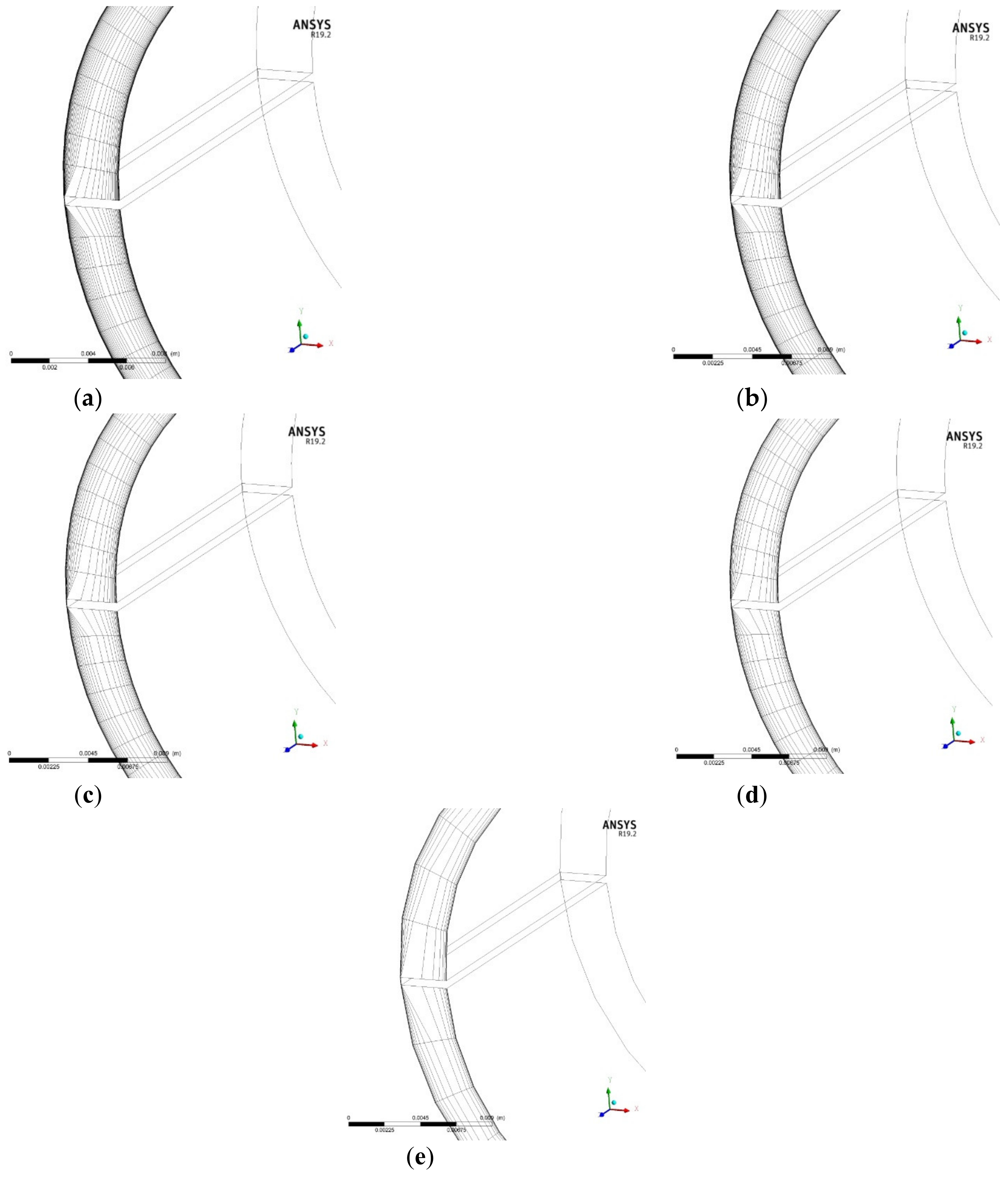
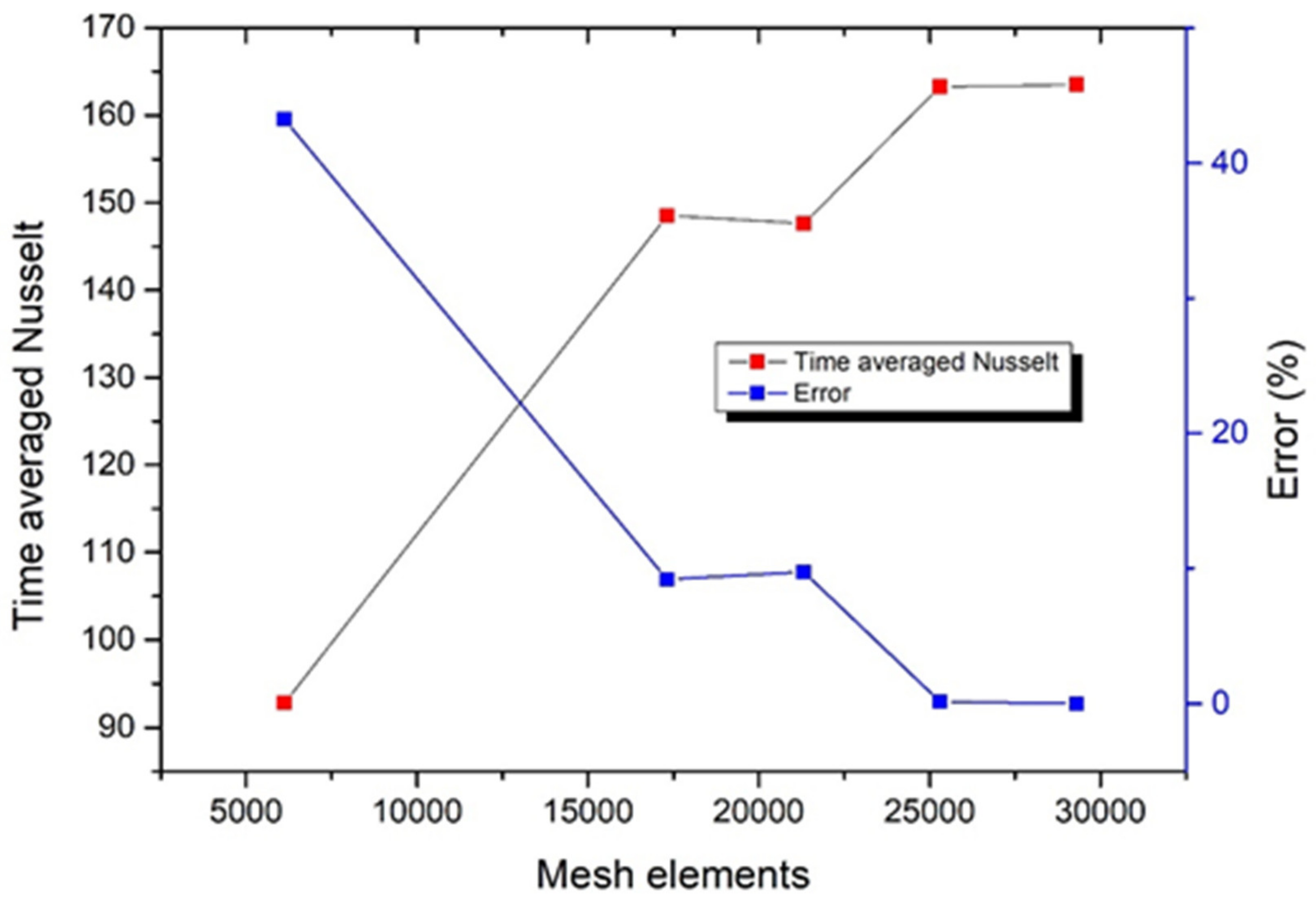
4.4. Numerical Detail

Special attention was paid to the generation of an appropriate numerical mesh that could be used in calculations. Three key objectives were established: high numerical mesh quality, accurate boundary layer resolution, and independence of mesh resolution from outcomes. Due to the complicated shape of the expander working chambers, it was not possible to achieve the high quality of all mesh cells (near 1.0). However, most of the mesh elements had a quality close to 1.0. The lowest numerical cell quality was 0.4 and was assigned to elements near the gap and vanes. To fulfil the second goal of high accuracy, very fine mesh had to be used near the walls surfaces. To achieve this, a non-uniform hexahedral mesh with the bigeometric law of node distribution was used [33]. Furthermore, to achieve the lowest value of y+ as possible, the distance of the first node from the wall was set at 2.5 µm. It allowed obtaining mean values of y+ close to 1 (listed in

Table 4. Properties of the working fluid (air) used in the simulations.

Mesh No.	Inlet Pressure (MPa) 1	y+ Mean (−)	y+ Max (−)
0	0.6	1.382	1.679
1	0.6	1.386	1.690
	0.5	1.224	1.467
	0.4	1.024	1.237
	0.3	0.827	1.004
	0.2	0.613	0.749
	0.1	0.383	0.466
2	0.6	1.411	1.701
3	0.6	1.400	1.695
4	0.6	1.112	1.300

¹ Gauge pressure.

). To obtain lower values of y+, the distance of the first node from the wall should be further lowered. However, for the mesh presented, it was not possible because it resulted in negative cell volumes during the mesh deformation.

In order to provide the mesh independence from the results, several simulations were performed on five meshes that differed in the number of cells. The selected meshes are shown in Figure 7, and the details of the distribution of the elements are collected in

Table 5. Properties of the working fluid (air) used in the simulations.

Mesh No.	Number of Elements
	Axially	Circumferentially	Gap	Vane	Total
0	9	76	22	22	29,304
1	9	76	19	19	25,308
2	9	76	16	16	21,312
3	9	76	13	13	17,316
4	9	44	10	10	6120

. To evaluate the numerical mesh, the most numerically unstable case was selected; that is, when the inlet pressure is the highest (0.6 MPa gauge pressure). Figure 8 shows the results of the mesh independence study for the mean Nusselt number on the inner cylinder wall. The Nusselt number was calculated according to Equation (17).

$$Nu=\frac{hD}{k\hspace{0.17em}}$$

(17)

where h, D, and k are the heat transfer coefficient at the inner cylinder wall, the inner diameter of the cylinder, and the thermal conductivity of the working fluid, respectively. The heat transfer coefficient was calculated according to Equation (18).

$$h=\left|\frac{q^{″}}{\Delta T}\right|$$

(18)

where q″ is the rate of heat transfer to the inner wall of the cylinder, and ΔT is the temperature difference formulated as Equation (19).

$$\Delta T={\overline{T}}_g-T_w$$

(19)

where ${\overline{T}}_g$ and $T_w$ are the average gas temperature inside the cylinder and the inner wall temperature of the cylinder, respectively. When the local Nusselt number was reached, the average value of the area was calculated using Equation (20).

$$N{u}_{av}=\frac{1}{A_{cyl}}{\displaystyle \underset{0}{\overset{A_{cyl}}{\int }}Nu\hspace{0.33em}\mathrm{d}A}$$

(20)

where A_cyl is the surface area of the inner cylinder wall. With the increase in mesh elements, the differences in the area-averaged Nusselt number in prescribed timesteps decrease. Regarding mesh no. 0 as exact, the results obtained for mesh no. 1 do not exceed 1%, while, for other meshes, they are much higher. For this reason, for further analyses, mesh no. 1 is considered to give accurate results in a reasonable time of calculation.

For the discretization of the advection terms, a High-Resolution scheme was used [32]. Transient terms were discretized with the use of the Second Order Backward Euler scheme. The residual target for all variables was set to 10⁻⁸ with the restriction of a maximum of 50 iterations per time step.

5. Results

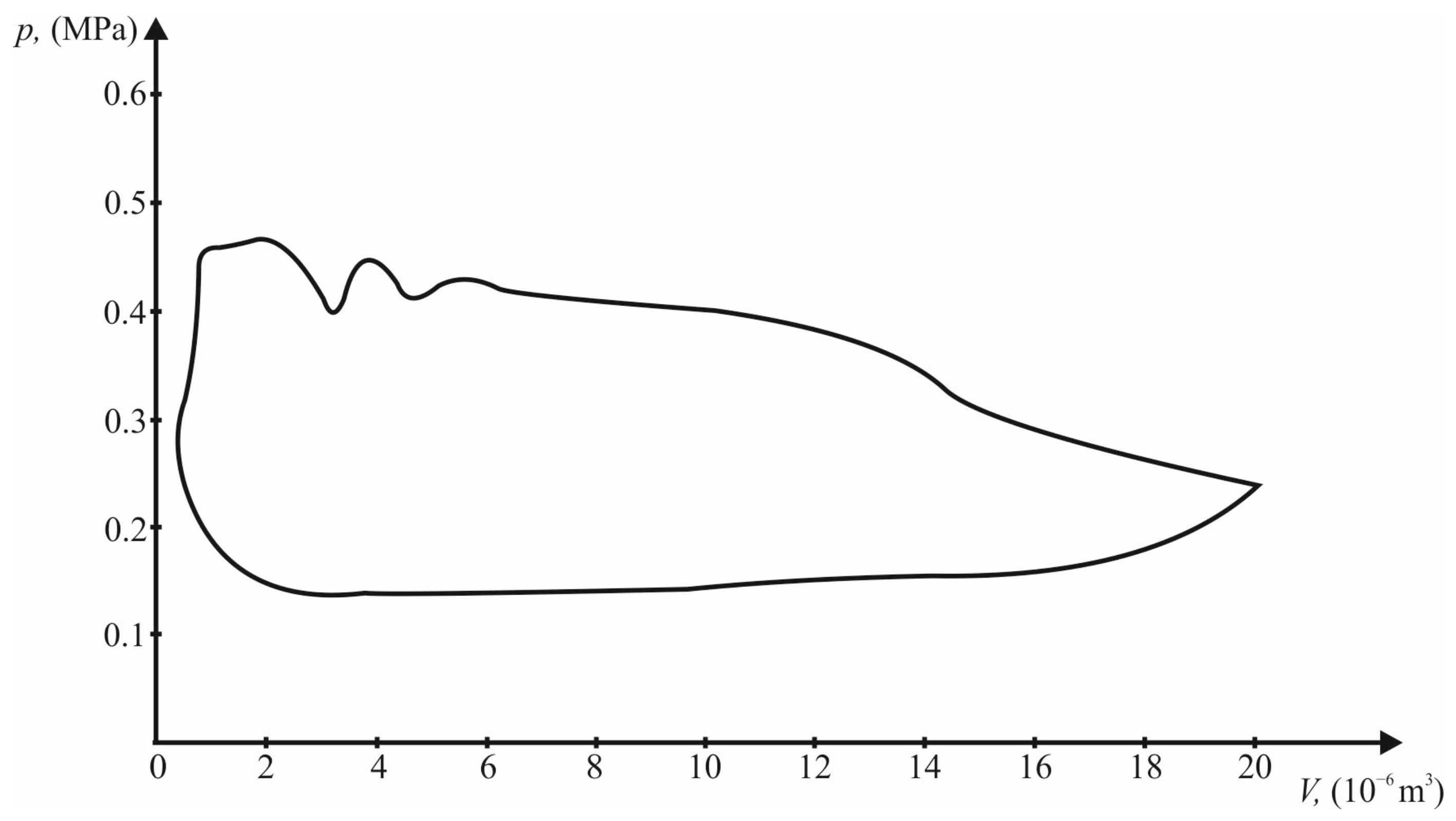
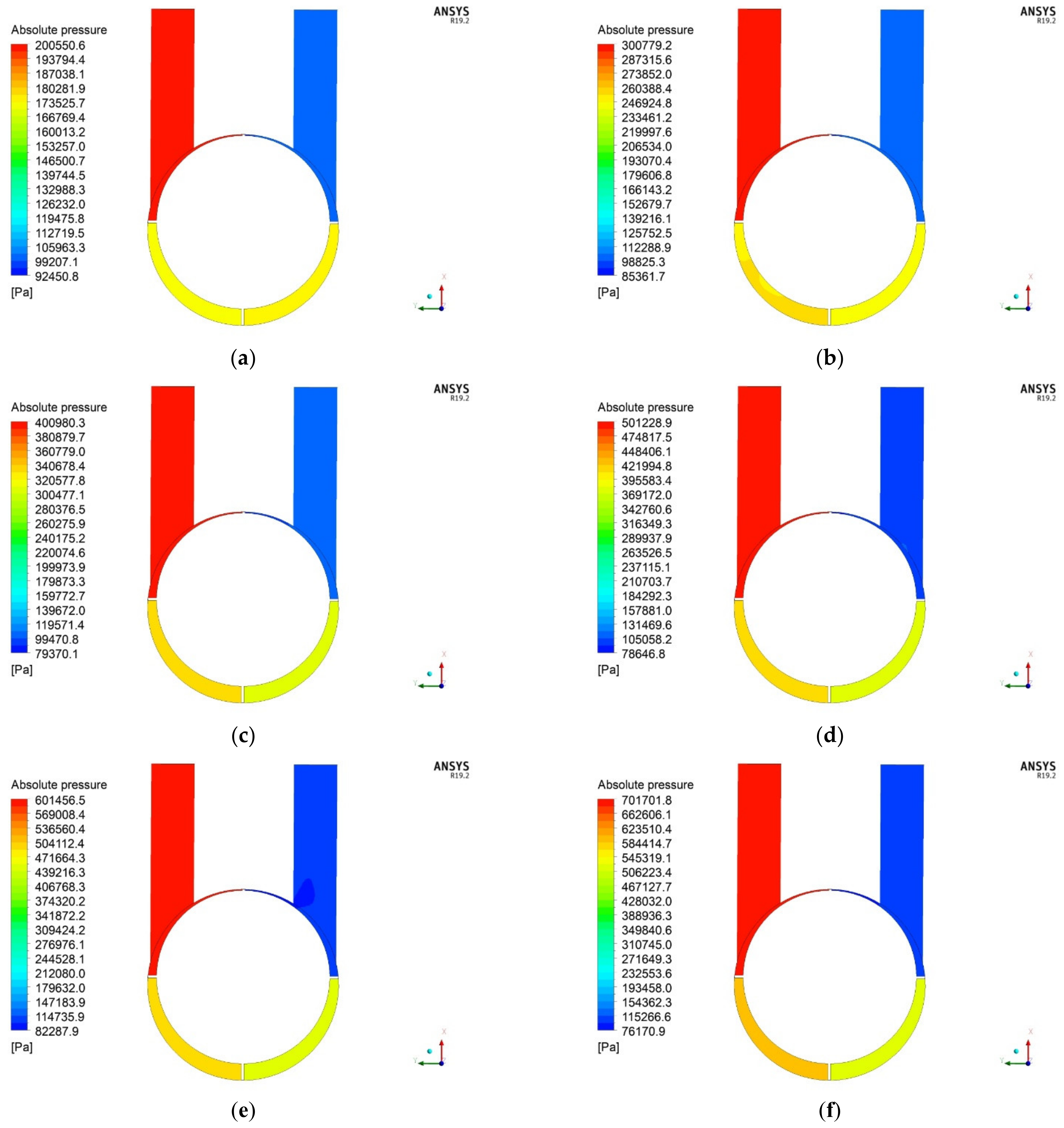
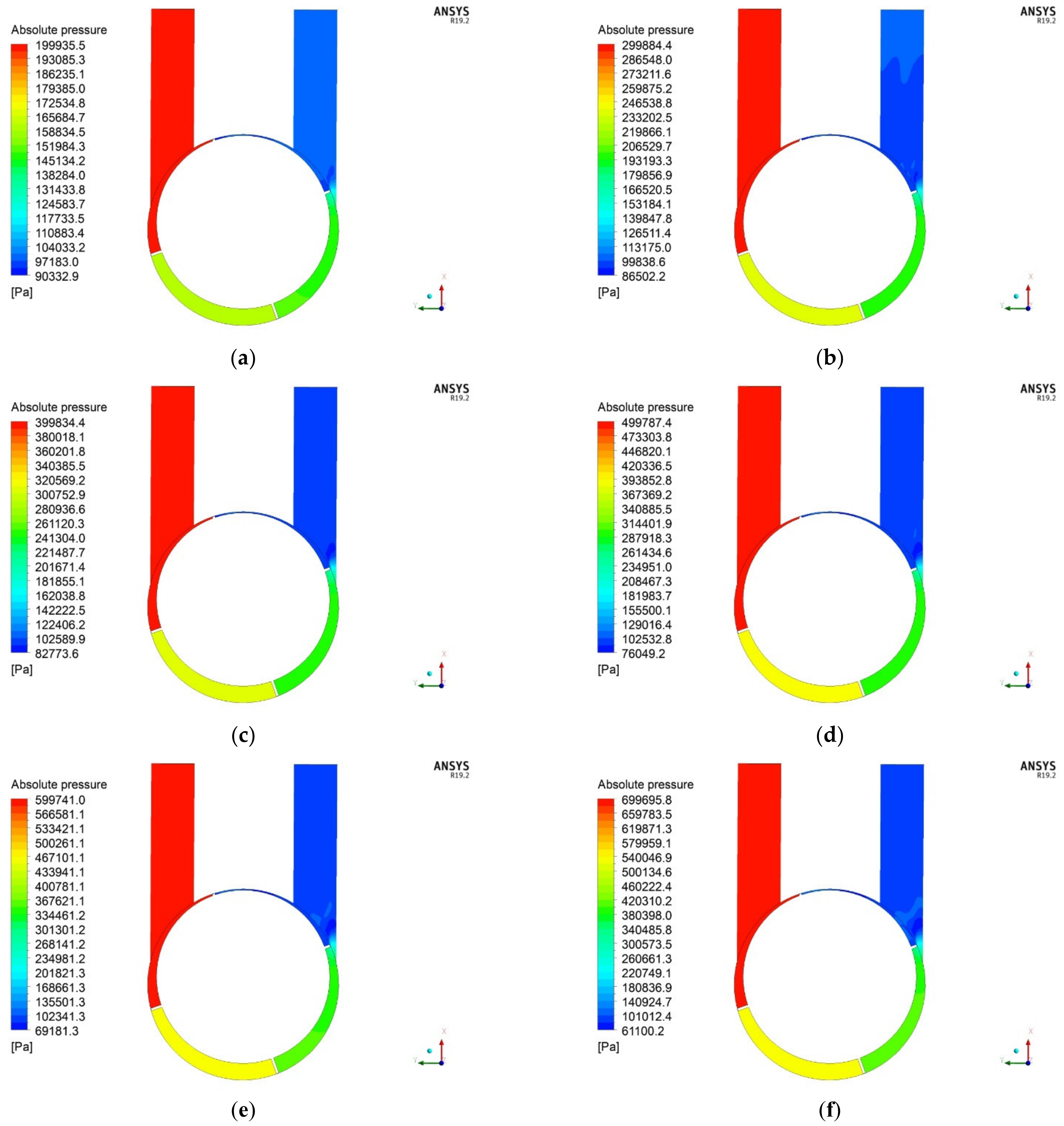
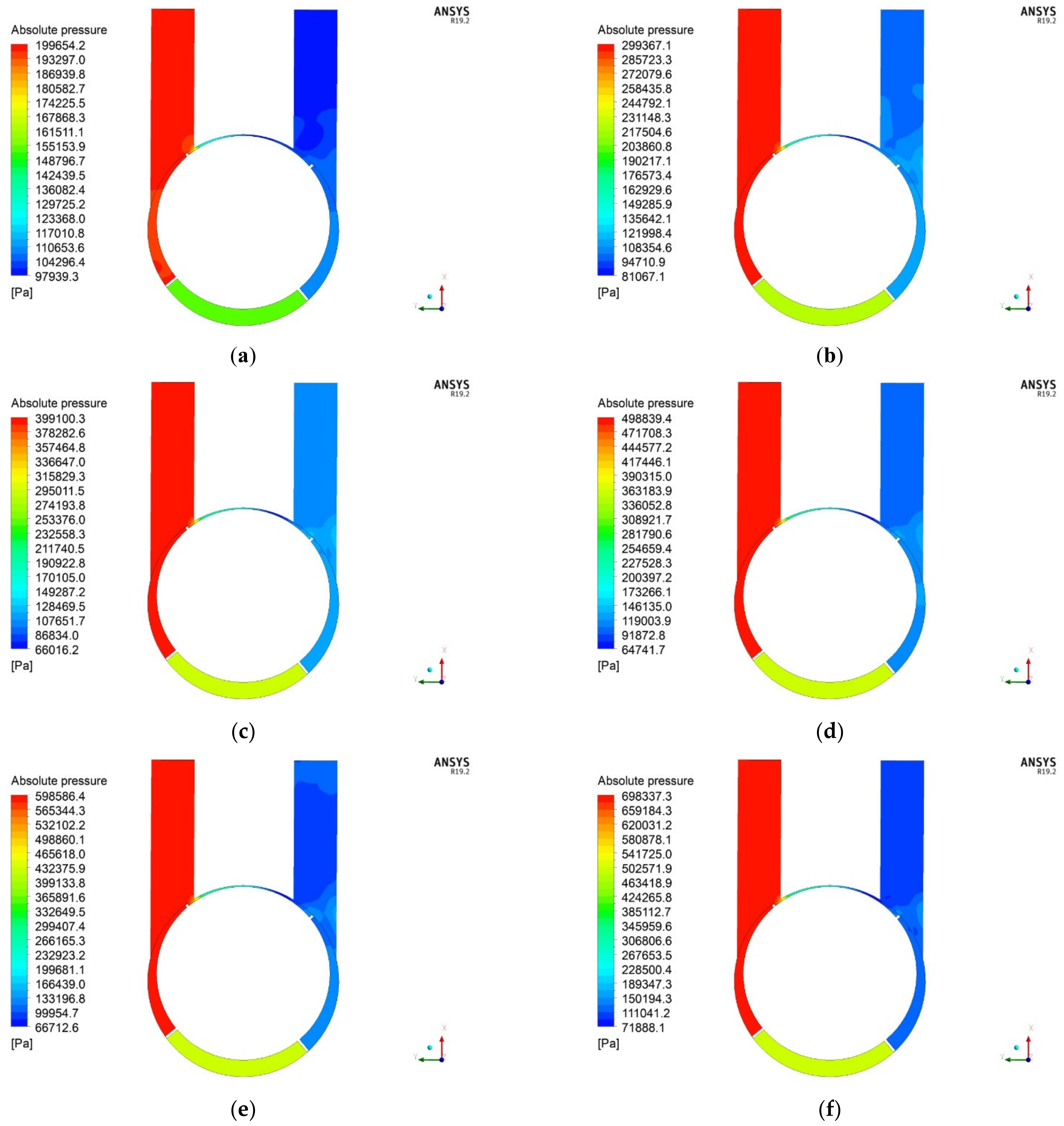
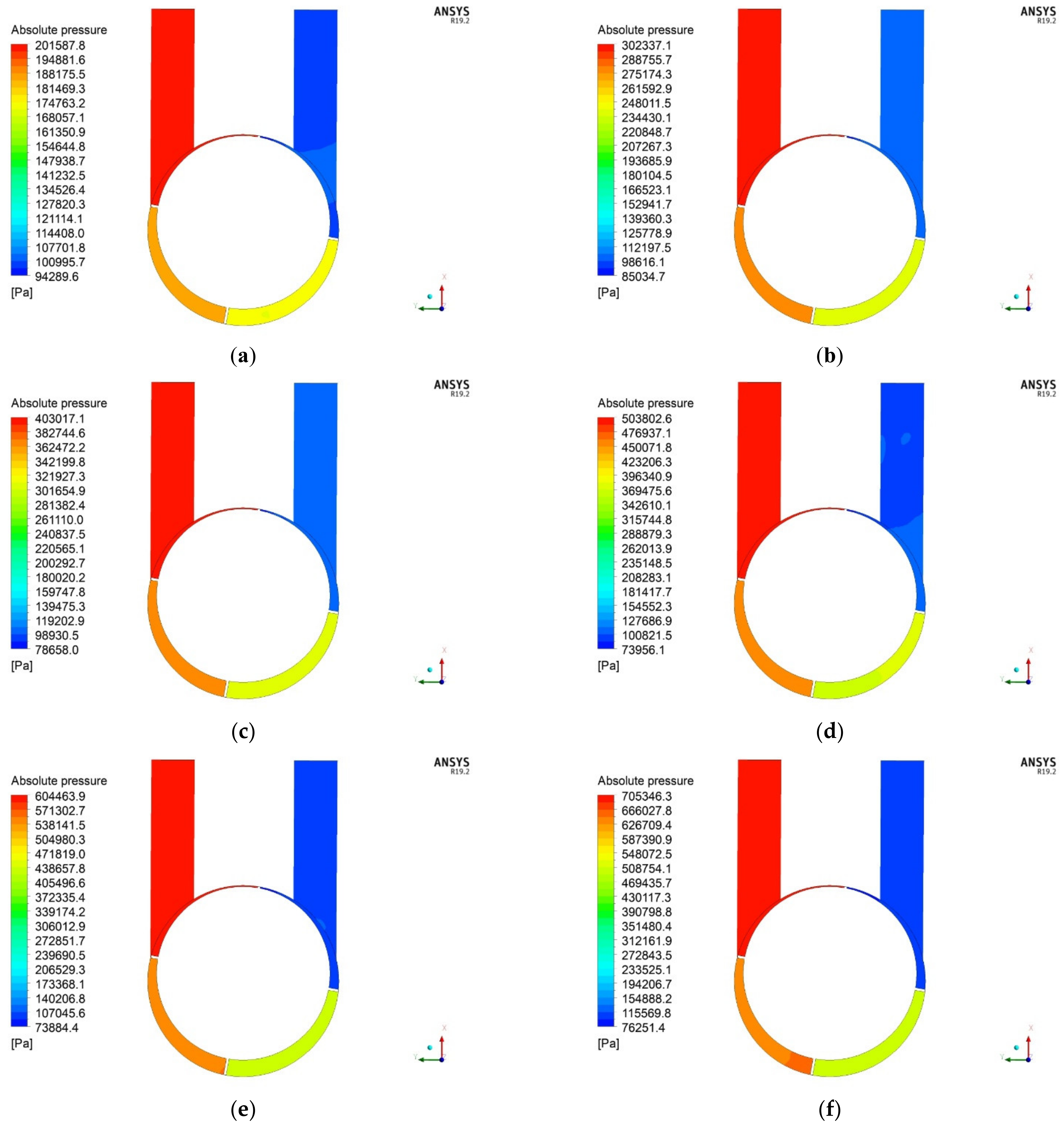
5.1. Distributions of Pressure

Figure 9, Figure 10, Figure 11, Figure 12 and Figure 13 show the absolute pressure distributions inside the expander for different total gauge pressures at the inlet and rotor rotation angles of the rotor in the range of 0° to 80°. The first thing to observe is that, despite the 40 µm gap between the cylinder wall and the tip of the vane, the working chambers are clearly separated. In each working chamber, the pressure is uniformly distributed, and it decreases with increasing rotor rotation angle. When the vanes move near to the slots of the inlet and outlet ports, the areas of high and low pressures are immediately connected (depicted in Figure 10 and Figure 11). This results in high perturbations and disruptions in the pressure field in these areas. This phenomenon is especially adverse near the 40° rotor rotation angle (see Figure 11) because the inlet and outlet ports are instantaneously connected, which declines the efficiency of the expander.

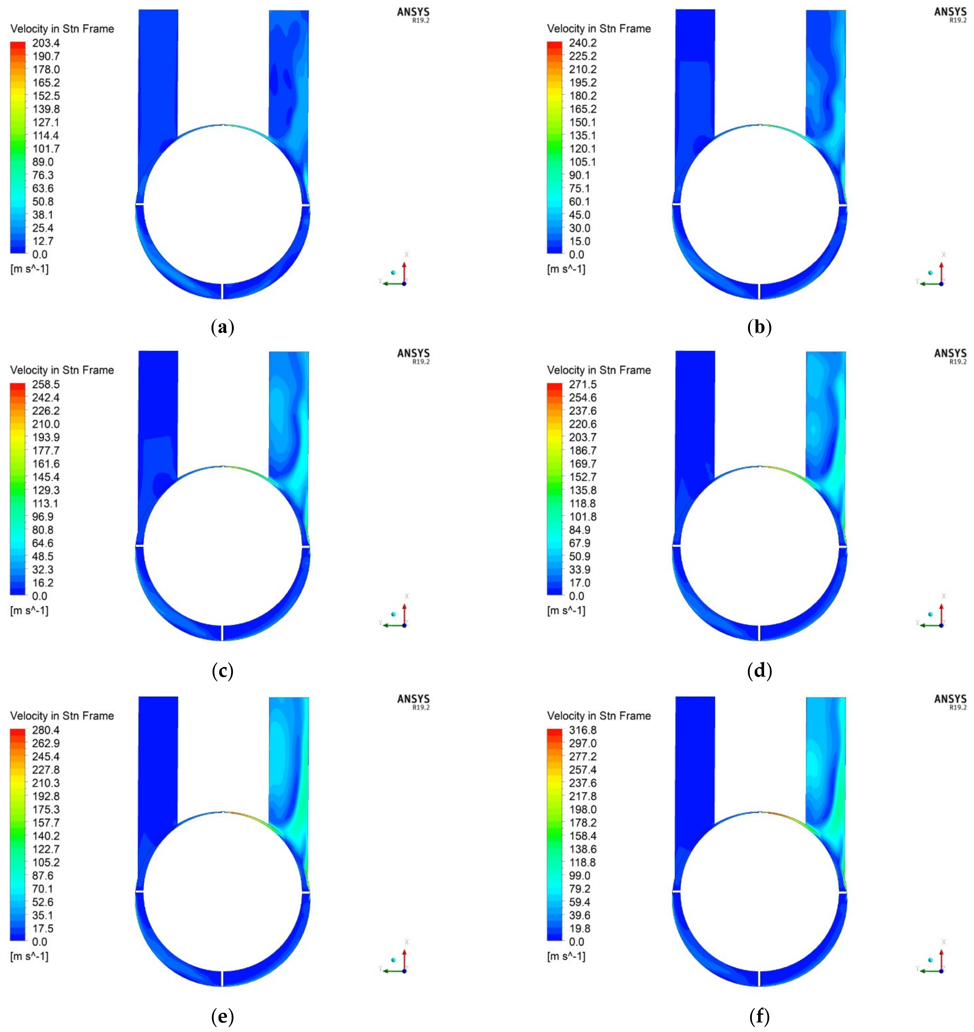
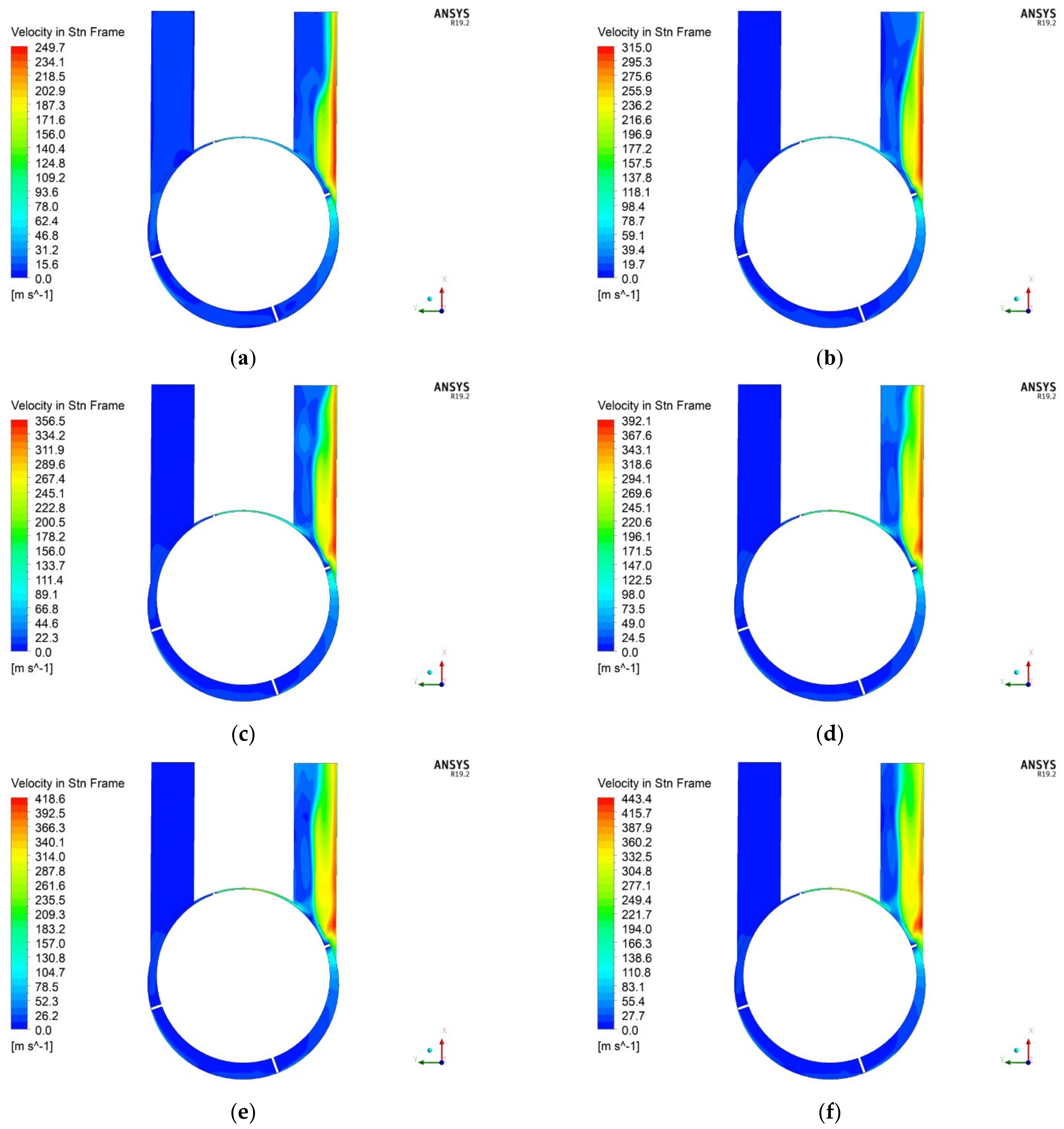
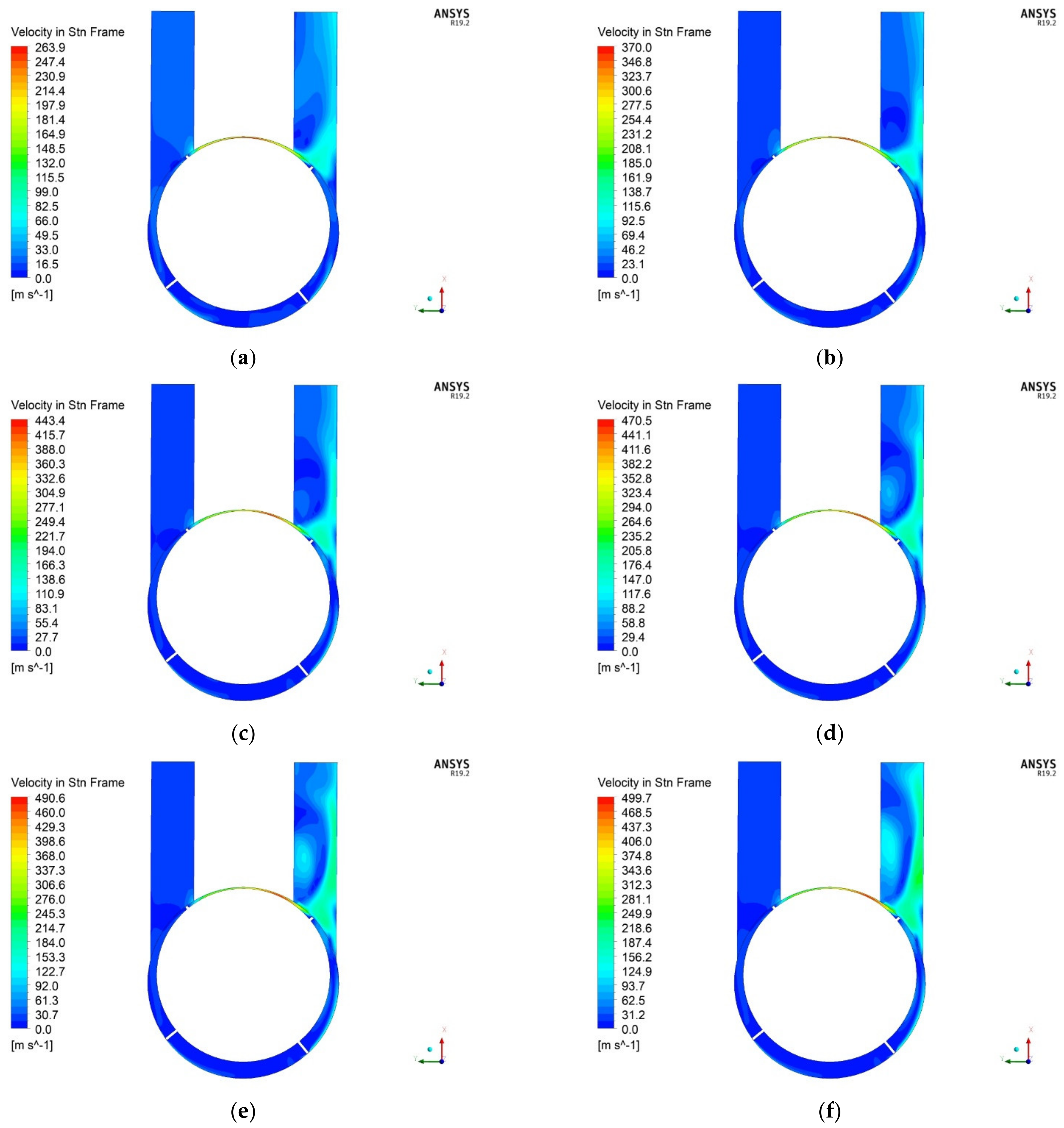
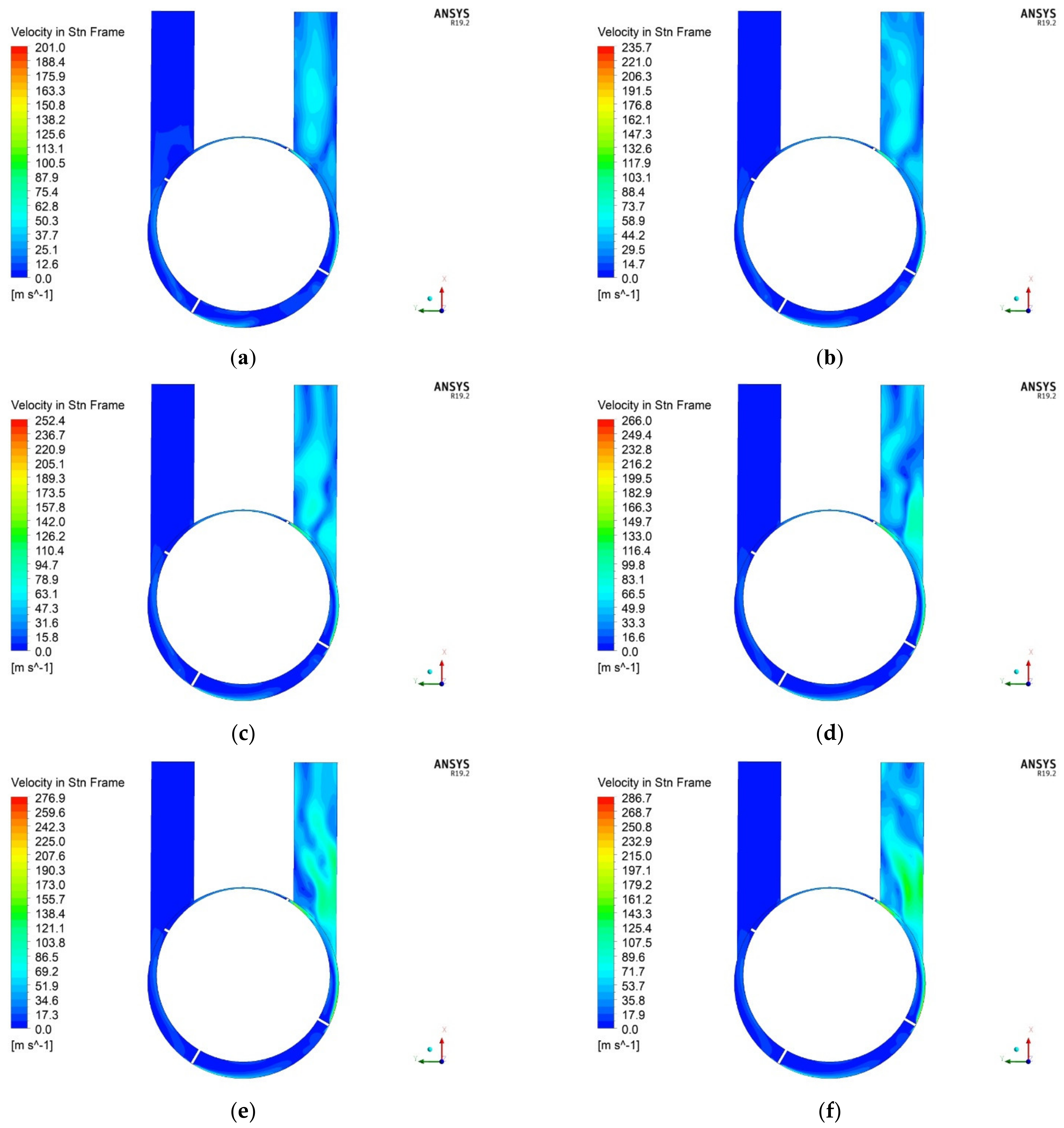
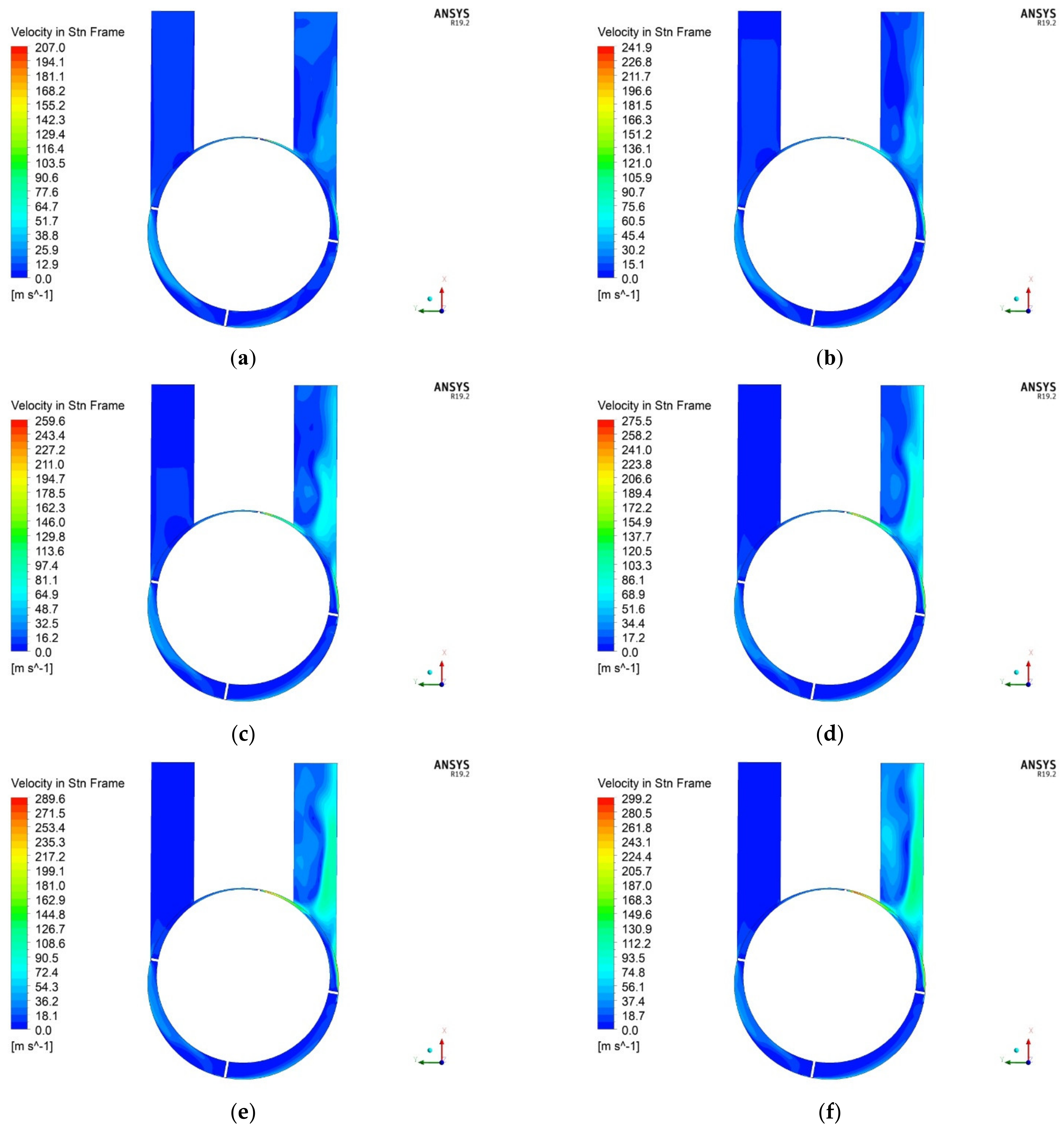
5.2. Distributions of Velocity

Figure 14, Figure 15, Figure 16, Figure 17 and Figure 18 present velocity distributions in stationary reference frames for different inlet total gauge pressures and rotor rotation angles varying in the range of 0–80°. In the case of a 0° rotor rotation angle, the velocity distribution is almost uniform in most working chambers. The exception is the last working chamber and the outlet port, where the lowest pressure prevails, as shown in Section 5.1. However, it can be seen that in the second working chamber, slight velocity variations are present. They are caused by the leakage between the first and the second working chamber triggered by large pressure differences (see Figure 9). Additionally, due to high pressure differences between the working chambers, especially between the first and fourth, leakages of the working fluid appear through the gap between the cylinder wall and the tip of the vane. This phenomenon greatly influences the velocity distribution, resulting in a drastic increase in velocities, notably near the tip of the vane in the last working chamber. Correspondingly, in the outlet port, a complex flow field develops with a recirculation zone. The maximum velocities emerge at the top of the expander near the vane that separates the first and fourth working chambers because the pressure difference is the highest there. This difference increases with increasing inlet pressure, and, for the limiting case of 0.6 MPa, the velocity approaches over 300 m/s.

The velocity also increases when the vanes move forward. A change in rotor rotation angle by 20° (see Figure 15) results in an enlarging of the area of high velocities in the outlet port. The velocity approaches even more than 400 m/s, but now, the maximum occurs on the right side of the outlet port wall, where most of the working fluid is impinged from the large hole opened by the moving vane. It can be seen that an increase in pressure from 0.1 to 0.6 MPa results in a rise of maximum velocity from 250 to 440 m/s. In the case of the 40° of rotation angle, the inlet and outlet ports are connected (illustrated in Figure 16), and the velocity rises further and reaches maximum values of almost 500 m/s in the case of the highest inlet pressure. It is also visible that, with increasing velocity, the vortex structure develos in the outlet port tube. It results in a nonuniform velocity field in this area that can cause a drop in efficiency [17,18]. With further movement of the vanes (see Figure 17), the velocity declines because the inlet and outlet ports are no longer connected and the working fluid can only flow through the vane tip-to-wall gap. Higher velocities are also observed near the gap between the second and third working chambers. Due to the connection of the inlet port and the second working chamber at this stage, a lower and uniformly distributed velocity field is formed there. Finally, at the end of this cycle (depicted in Figure 18) a slight increase in maximum velocities is observed behind the vane that separates the first and last working chamber. In this position, a high pressure difference between these chambers appears and results in leakage driven by large velocities.

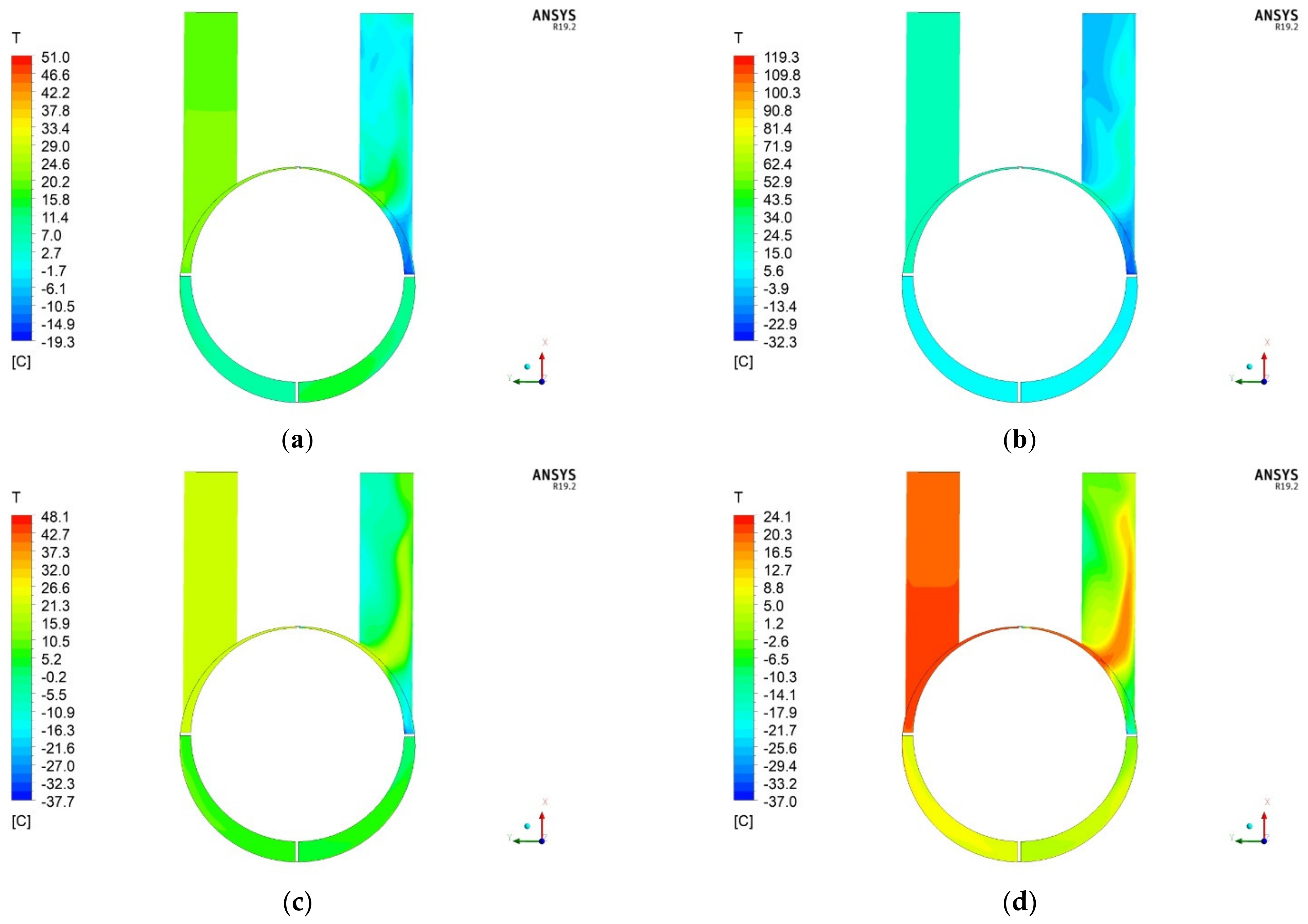
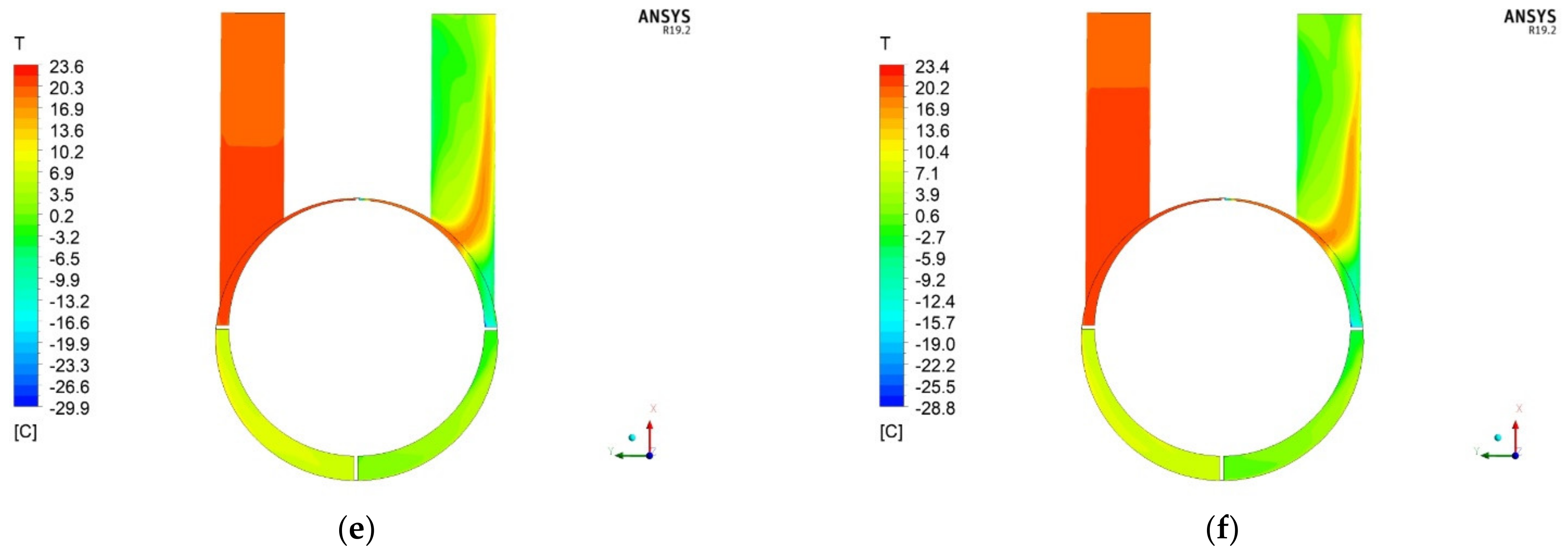
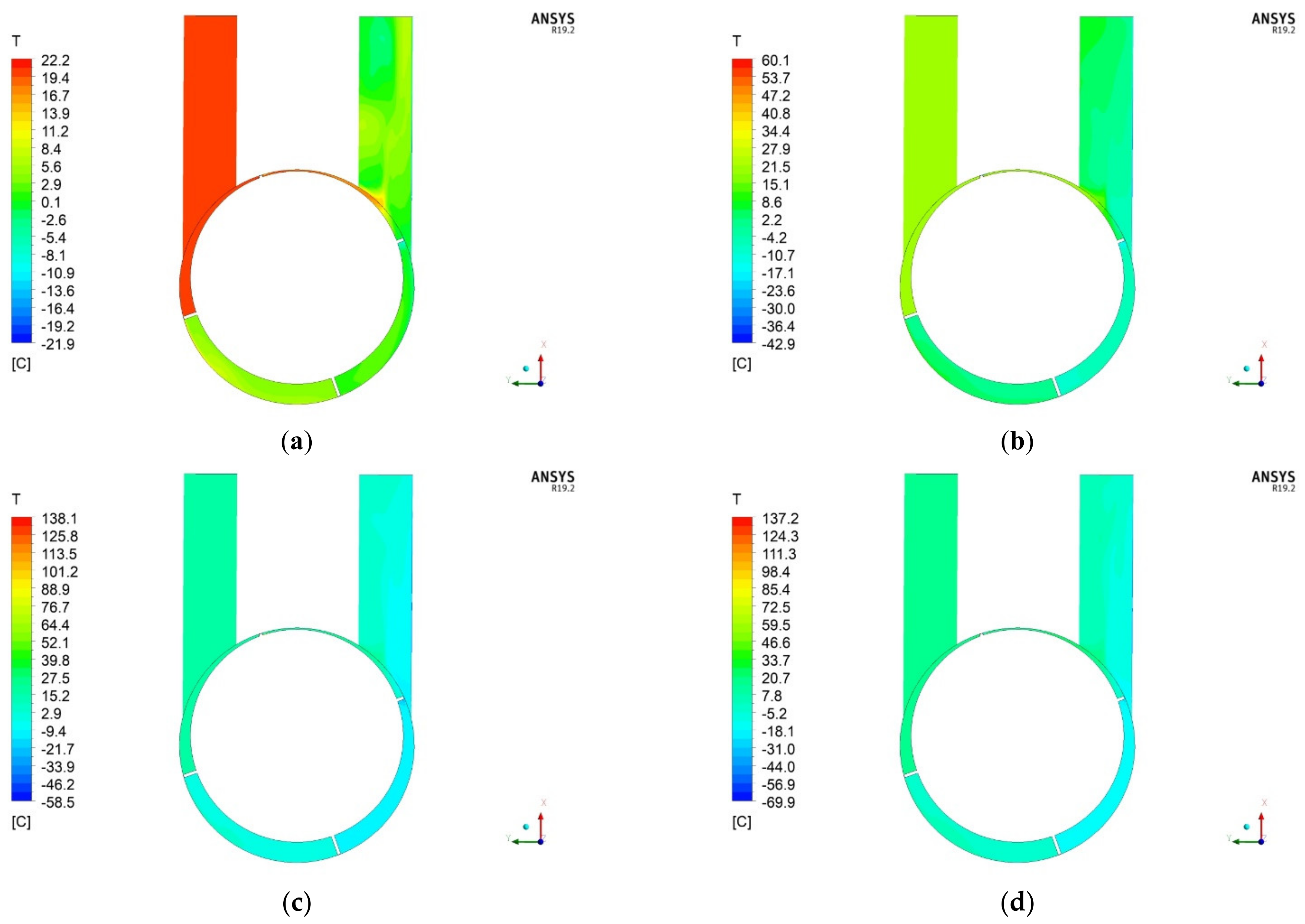
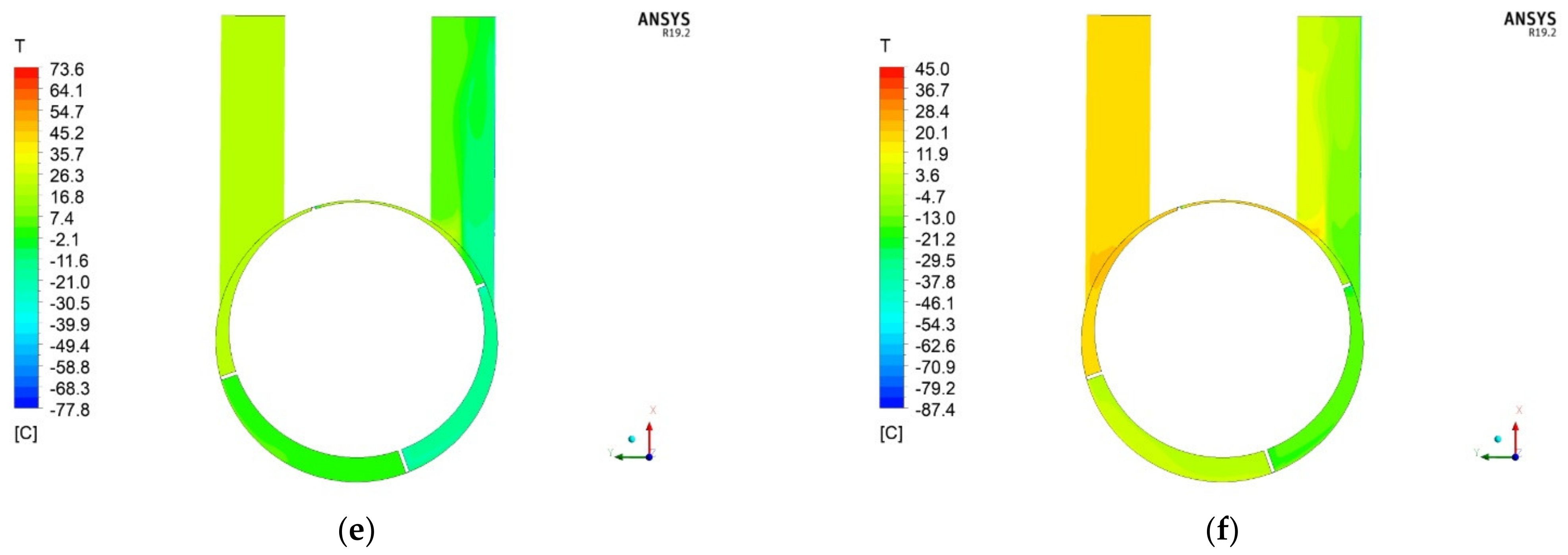
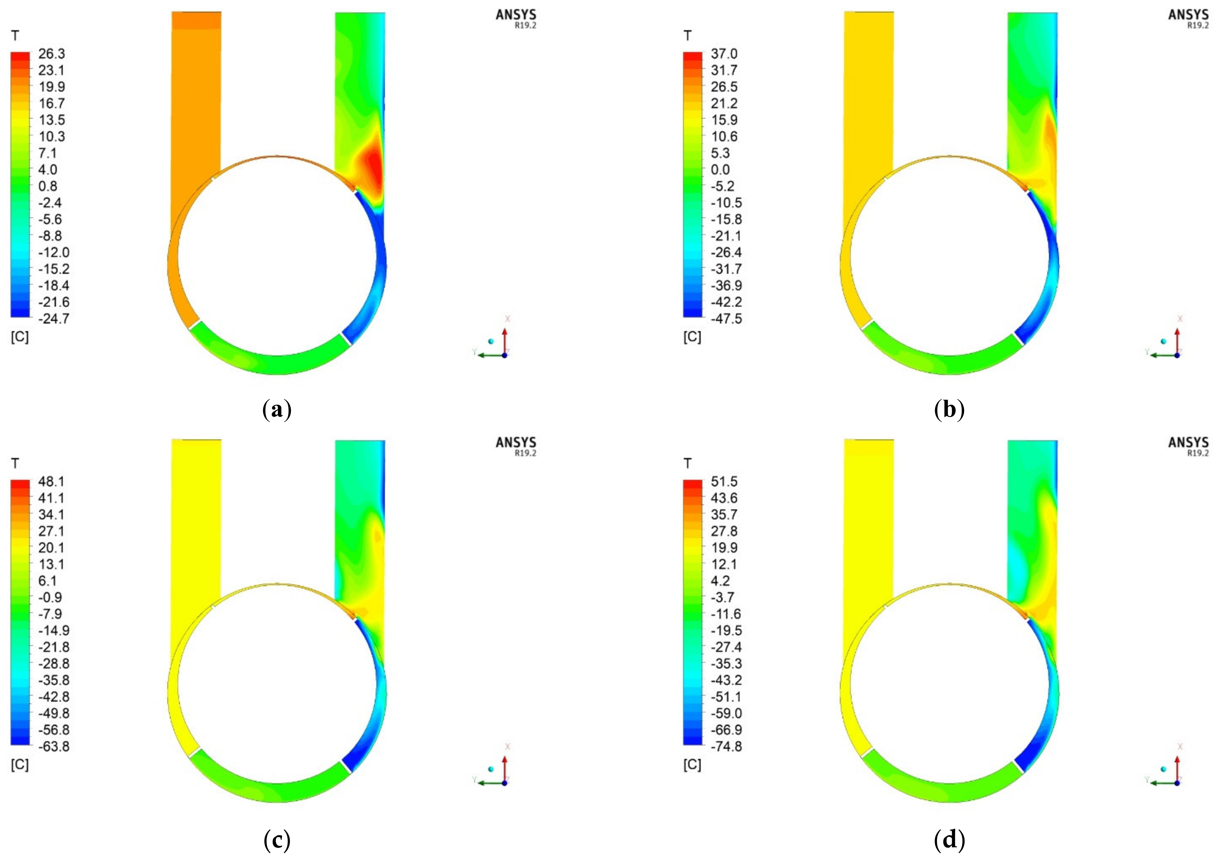
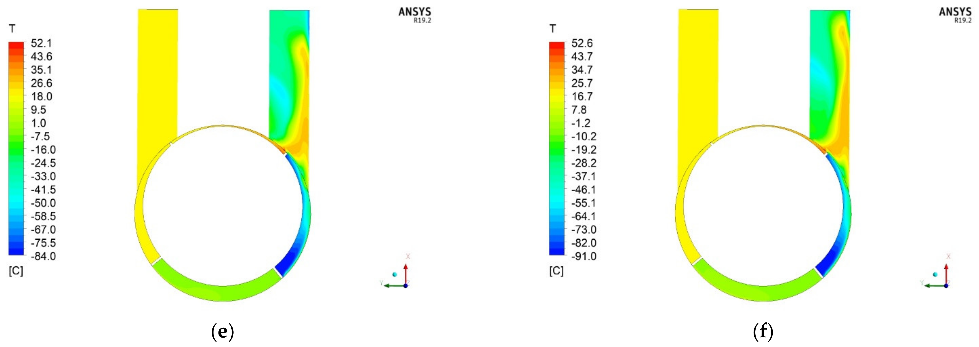
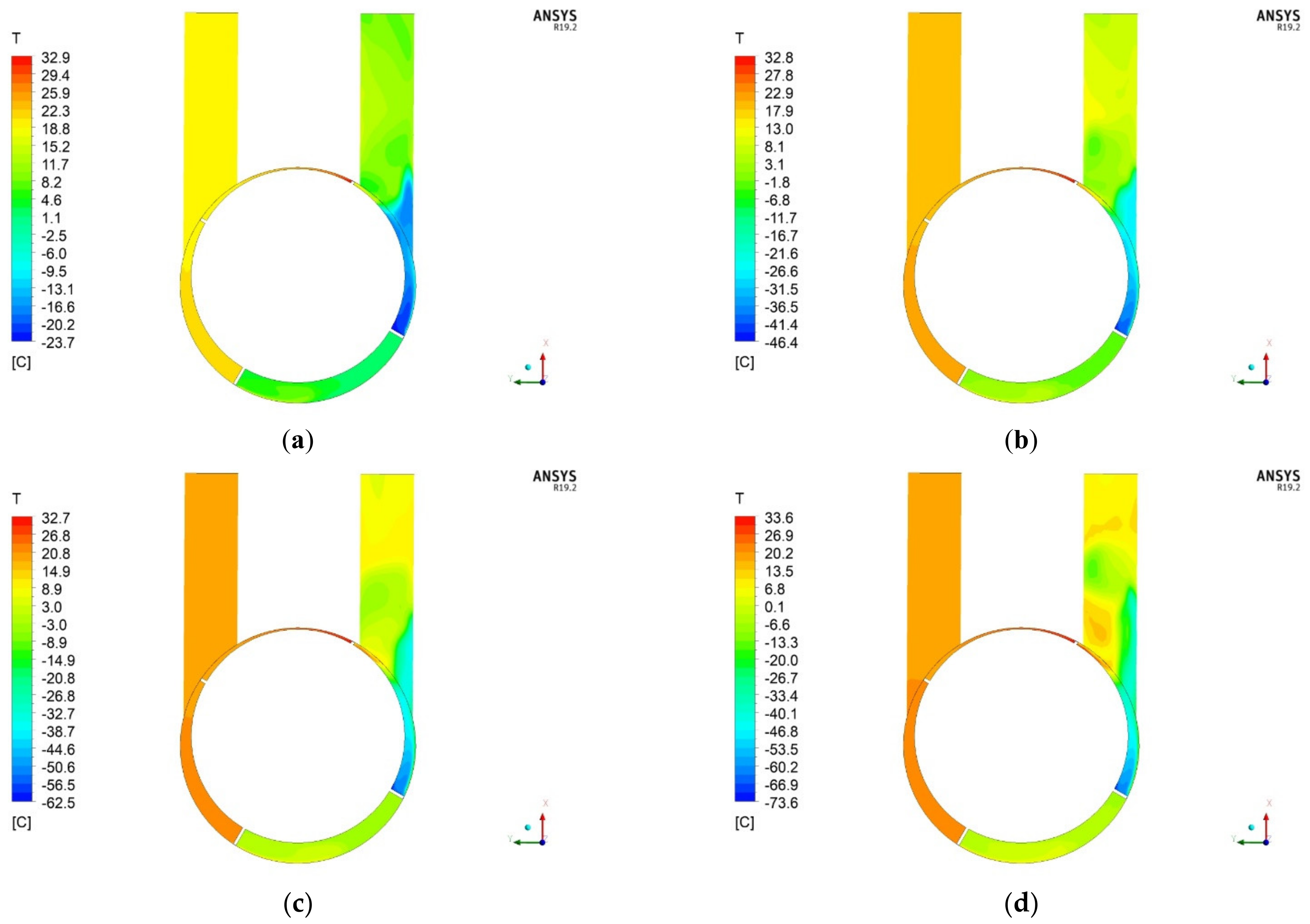
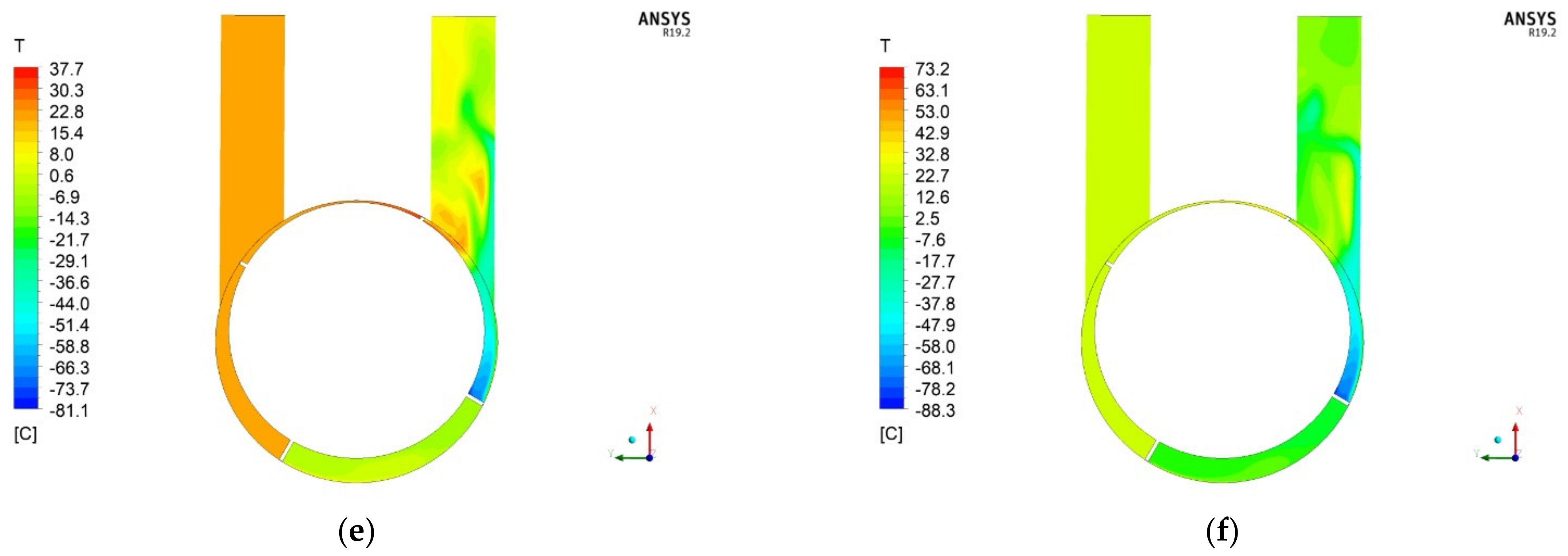
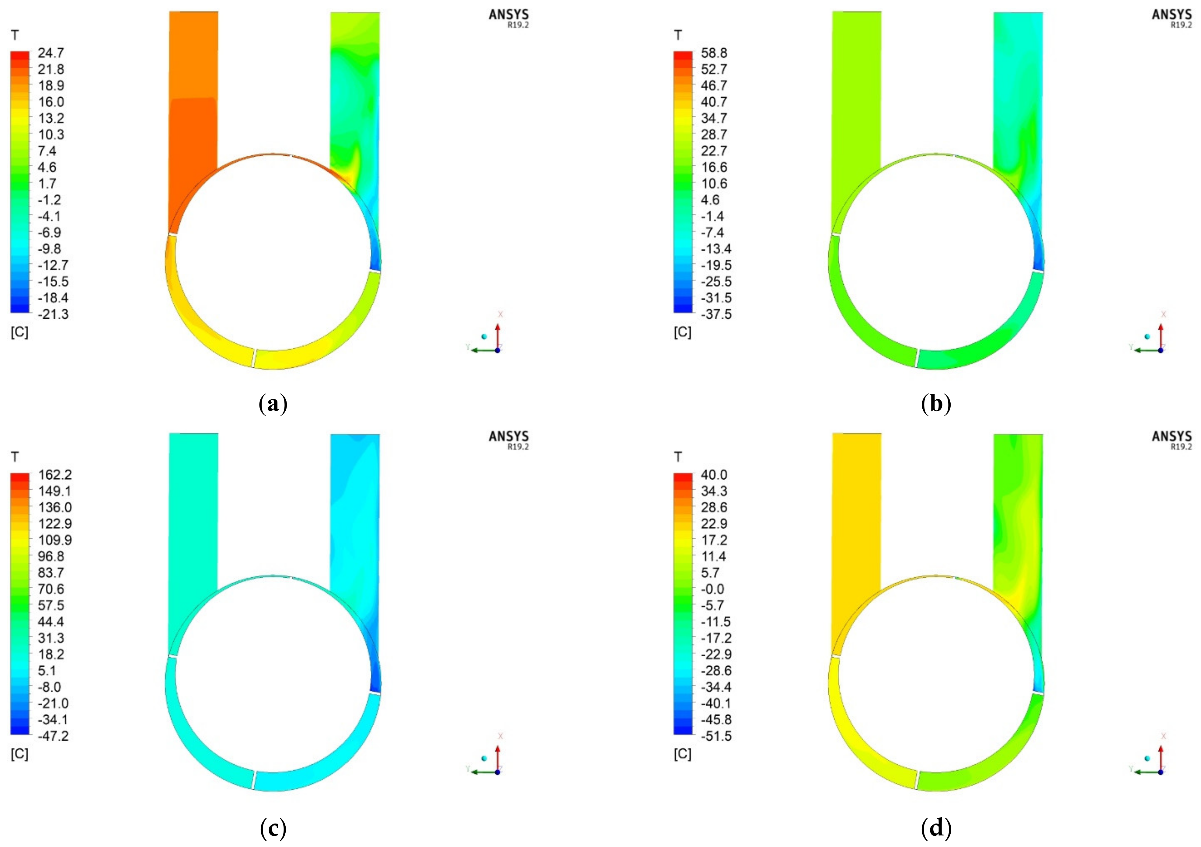
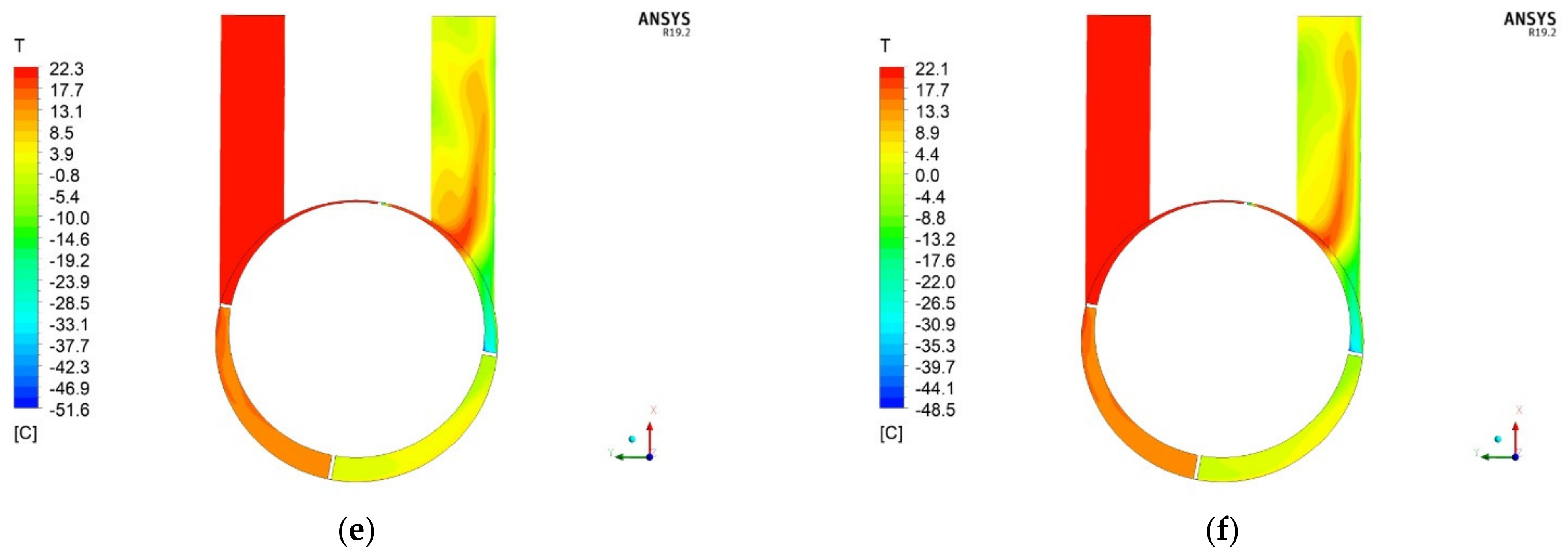
5.3. Distributions of Temperature

The variations in the velocity field presented in Section 5.2 have a direct reflection on the temperature field. Figure 19, Figure 20, Figure 21, Figure 22 and Figure 23 show temperature distributions in the expander for different inlet pressures and rotor rotation angles changed from 0° to 80°. The working fluid expands in the working chambers and its temperature decreases downward. Similar to the velocity field, the temperature field is almost uniformly distributed in the working chambers, except for the last one. Leakages cause the mixing of hot air from the working chambers with high pressures, and thus temperatures with colder air in the last working chamber. It strongly disrupts the temperature distribution in this area.

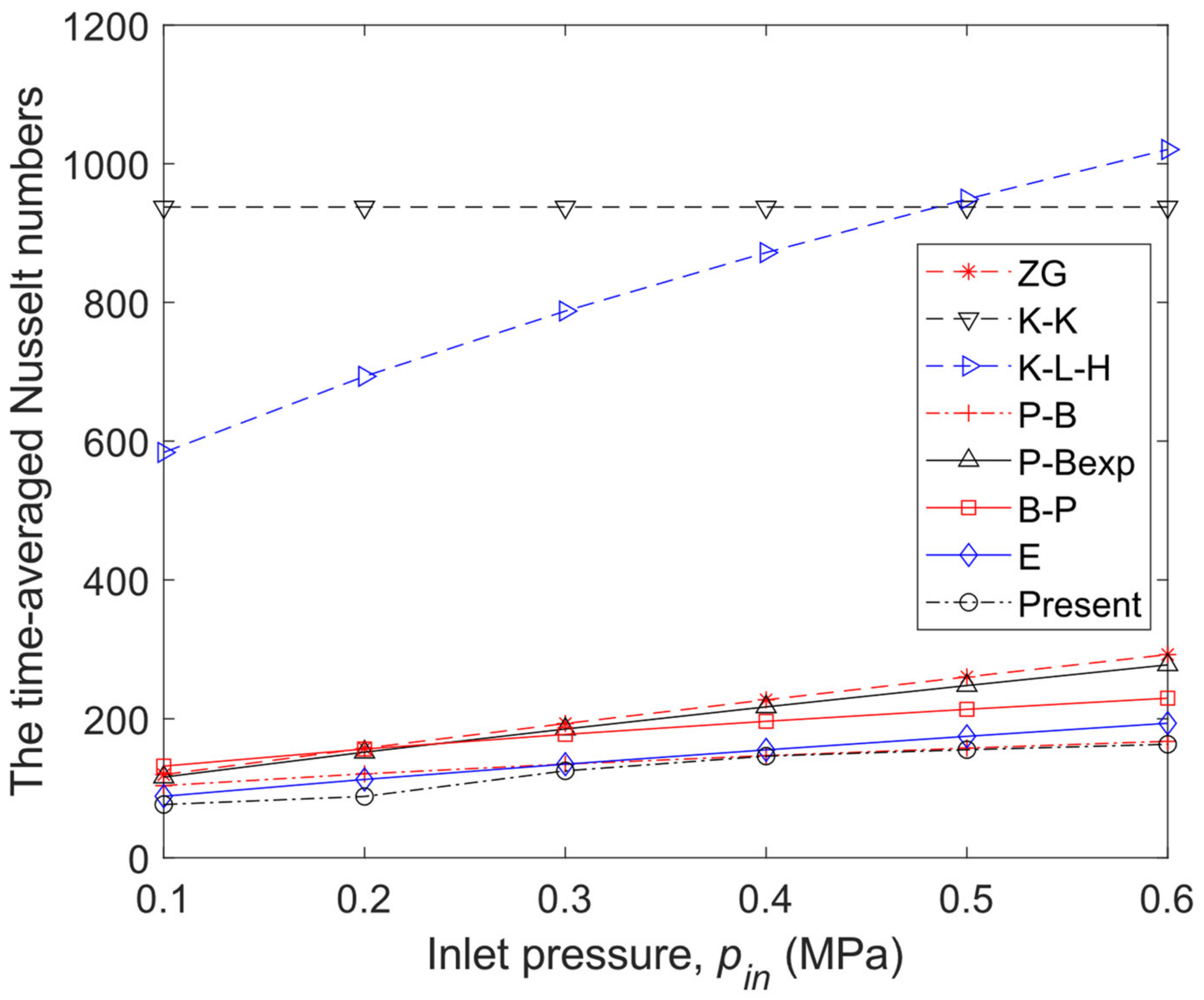
5.4. Comparison of the Nusselt Number with Available Correlations

In order to compare the numerically obtained Nusselt numbers with existing correlations from the literature, the time-averaged Nusselt number was calculated. The results of the comparison are shown in

Table 6. Comparison of the time-averaged Nusselt numbers obtained from the present model and selected correlations.

Model
Inlet Pressure (MPa)	ZG [20]	K-K [20]	K-L-H [20]	P-B [20]	P-Bexp [20]	B-P [20]	E [20]	Present
0.1	119.6	937.5	583.6	103.8	116.1	131.9	88.5	76.6
0.2	157.6	937.5	693.4	120.8	152.0	156.5	112.7	88.2
0.3	193.2	937.5	787.5	134.8	185.3	177.6	134.7	125.1
0.4	227.3	937.5	871.8	147.0	217.2	196.4	155.3	146.3
0.5	260.4	937.5	948.9	157.8	247.9	213.7	174.8	155.5
0.6	292.5	937.5	1020.5	167.6	277.7	229.7	193.6	163.3

and illustrated in Figure 24. Furthermore, the calculated value of the mean absolute percentage error (MAPE) is listed in

Table 7. Comparison of the time-averaged Nusselt numbers with regard to the presented study.

Parameter	ZG	K-K	K-L-H	P-B	P-Bexp	B-P	E
MAPE	65%	709%	568%	14%	58%	51%	15%

to represent the statistical analysis of each model with respect to the presented study. The K-K and K-L-H models give higher values of the Nusselt number compared to other models, and, in this case, the K-K and L-H models present the bigger MAPE (see Figure 24 and Table 7). Despite the fact that the ZG, P-B, P-B_exp, B-P, and E models give almost similar results, it appears that the model of ZG, P-B, and P-B_exp still obtains a relatively higher error (MAPE of more than 50%). Moreover, all of the results from the literature are close to the present results. The results obtained are more comparable to the results modeled using E and PB models that are presented in Table 7 by MAPE of 15% and 14%, respectively (especially for an inlet pressure greater than 0.2 MPa). It suggests that the heat transfer mechanism is different in MVEs than in the case of other machines and devices with rotating vanes, and further work on this topic should be focused on experimental analyses of the heat exchange in these machines.

6. Conclusions

In the present article, an improved numerical model of heat transfer and fluid flow inside an MVE was shown. The principle of operation of the MVE was first stated. Then, a detailed analysis of heat transfer that occurs in such a machine was given. In the work, special attention was paid to improving previous models of the authors to accurately model heat transfer phenomena inside the MVE. To the knowledge of the authors, this is the first numerical attempt to model heat transfer in MVE, and this is the state of the art feature of this investigation. The numerical mesh was also thoroughly improved, providing mesh independence and y+ values close to 1. The simulations covered the total relative inlet pressures in a range of 0.1–0.6 MPa. The results were presented as pressure, velocity, and temperature distributions in terms of inlet pressure and rotor rotation angle. Moreover, the average Nusselt number on the inner cylinder wall that is scraped by rotating vanes was calculated. The main findings can be drawn as follows:

• The transient results of the Nusselt number showed a periodic maximum that occurs near 30° of rotor rotation.
• The time-averaged Nusselt number was compared with available correlations from the literature, and the results were most comparable to the results modeled using E and P-B models (especially for inlet pressure higher than 0.2 MPa), that the MAPE of E and P-B models, with regard to the presented study, indicate 15% and 14%, respectively.
• A comparison of the modeling results suggested that the applicability of models which are available in the literature and are applied for modeling the heat transfer in other machines and devices with rotating vanes (e.g., scraped surface heat exchangers) is limited in the case of estimating the heat transfer processes in a multi-vane machine. This can be caused by the different intensities of the thermal and flow processes that occur during the expansion of gas in the expander working chambers and the higher rotational speeds of the shaft.
• The numerical results indicated that the flow is characterized by high velocities and intensive mixing of the working fluid.
• Leakages of the working fluid between adjacent working chambers influence the flow of the working fluid and, therefore, the heat transfer conditions.

In summary, further works should focus on experimental research on heat transfer conditions in these types of machines and develop Nusselt number correlations, which are specifically valid for MVEs.

References

1. Gnutek, Z.; Kolasiński, P. The Application of Rotary Vane Expanders in Organic Rankine Cycle Systems—Thermodynamic Description and Experimental Results. J. Eng. Gas Turbines Power 2013, 135, 061901. [Google Scholar] [CrossRef]
2. Kolasinski, P. Application of the Multi-Vane Expanders in Orc Systems—A Review on the Experimental and Modeling Research Activities. Energies 2019, 12, 2975. [Google Scholar] [CrossRef] [Green Version]
3. Hanson, K. Prototype Solar Heating and Combined Heating and Cooling Systems (Quarterly Report No. 3); DTIE (Divison of Technical Information Extension, US Atomic Energy Commission): Washington, DC, USA, 1977. [Google Scholar] [CrossRef] [Green Version]
4. Badr, O.; O’Callaghan, P.W.; Hussein, M.; Probert, S.D. Multi-Vane Expanders as Prime Movers for Low-Grade Energy Organic Rankine-Cycle Engines. Appl. Energy 1984, 16, 129–146. [Google Scholar] [CrossRef]
5. Badr, O.; Probert, S.D.; O’Callaghan, P. Performances of Multi-Vane Expanders. Appl. Energy 1985, 20, 207–234. [Google Scholar] [CrossRef]
6. Badr, O.; O’Callaghan, P.W.; Probert, S.D. Rankine-Cycle Systems for Harnessing Power from Low-Grade Energy Sources. Appl. Energy 1990, 36, 263–292. [Google Scholar] [CrossRef]
7. Badr, O.; Probert, S.D.; O’Callaghan, P.W. Selecting a Working Fluid for a Rankine-Cycle Engine. Appl. Energy 1985, 21, 1–42. [Google Scholar] [CrossRef]
8. Badr, O.; O’Callaghan, P.W.; Probert, S.D. Thermodynamic and Thermophysical Properties of Organic Working Fluids for Rankine-Cycle Engines. Appl. Energy 1985, 19, 1–40. [Google Scholar] [CrossRef]
9. Badr, O.; Hussein, M.; Probert, S.D.; O’Callaghan, P.W. Thermal Stabilities of Mixtures of Trichlorofluoroethane and Lubricating Fluids Contained in Copper Sealed Tubes. Appl. Energy 1984, 16, 41–52. [Google Scholar] [CrossRef]
10. Badr, O.; O’Callaghan, P.W.; Probert, S.D. Performances of Rankine-Cycle Engines as Functions of Their Expanders’ Efficiencies. Appl. Energy 1984, 18, 15–27. [Google Scholar] [CrossRef]
11. Badr, O.; Probert, S.D.; O’Callaghan, P. Multi-Vane Expanders: Vane Dynamics and Friction Losses. Appl. Energy 1985, 20, 253–285. [Google Scholar] [CrossRef]
12. Badr, O.; Probert, S.D.; O’Callaghan, P.W. Multi-Vane Expanders: Internal-Leakage Losses. Appl. Energy 1985, 20, 1–46. [Google Scholar] [CrossRef]
13. Badr, O.; O’Callaghan, P.W.; Probert, S.D. Multi-Vane Expander Performance: Breathing Characteristics. Appl. Energy 1985, 19, 241–271. [Google Scholar] [CrossRef]
14. Badr, O.; O’Callaghan, P.W.; Probert, S.D. Multi-Vane Expanders: Geometry and Vane Kinematics. Appl. Energy 1985, 19, 159–182. [Google Scholar] [CrossRef]
15. Gnutek, Z.; Kalinowski, E. Application of Rotary Vane Expanders in Systems Utilizing the Waste Heat. In Proceedings of the International Compressor Engineering Conference, Purdue University, West Lafayette, IN, USA, 19–22 July 1994. [Google Scholar]
16. Gnutek, Z. Sliding-Vane Rotary Machinery. Developing Selected Issues of One-Dimensional Theory; Wrocław University of Technology Publishers: Wrocław, Poland, 1997. [Google Scholar]
17. Rak, J.; Błasiak, P.; Kolasiński, P. Influence of the Applied Working Fluid and the Arrangement of the Steering Edges on Multi-Vane Expander Performance in Micro ORC System. Energies 2018, 11, 892. [Google Scholar] [CrossRef] [Green Version]
18. Kolasiński, P.; Błasiak, P.; Rak, J. Experimental and Numerical Analyses on the Rotary Vane Expander Operating Conditions in a Micro Organic Rankine Cycle System. Energies 2016, 9, 606. [Google Scholar] [CrossRef] [Green Version]
19. Kolasiński, P.; Pomorski, M.; Błasiak, P.; Rak, J. Use of Rolling Piston Expanders for Energy Regeneration in Natural Gas Pressure Reduction Stations—Selected Thermodynamic Issues. Appl. Sci. 2017, 7, 535. [Google Scholar] [CrossRef]
20. Błasiak, P.; Kolasiński, P.; Daniarta, S. Analysis of Heat Transfer within Rotary Vane Expander. In Proceedings of the 6th International Seminar on ORC Power Systems, Munich, Germany, 11–13 October 2021. [Google Scholar] [CrossRef]
21. Gnutek, Z. Gazowe Objętościowe Maszyny Energetyczne—Podstawy; Wrocław University of Science and Technology Publishing: Wrocław, Poland, 2004. [Google Scholar]
22. Mamontow, M. Voprosy Termodynamiki Tiela Pieremiennoj Massy; Obrongiz: Moscow, Russia, 1961. [Google Scholar]
23. Błasiak, P.; Pietrowicz, S. Towards a Better Understanding of 2D Thermal-Flow Processes in a Scraped Surface Heat Exchanger. Int. J. Heat Mass Transf. 2016, 98, 240–256. [Google Scholar] [CrossRef]
24. Błasiak, P.; Pietrowicz, S. An Experimental Study on the Heat Transfer Performance in a Batch Scraped Surface Heat Exchanger under a Turbulent Flow Regime. Int. J. Heat Mass Transf. 2017, 107, 379–390. [Google Scholar] [CrossRef]
25. Błasiak, P. Wpływ Zmiennych Warunków Ruchu Płynu w Pobliżu Ścianki Na Wymianę Ciepła. Ph.D. Thesis, Wrocław University of Science and Technology, Wrocław, Poland, 2015. [Google Scholar]
26. Kern, D.Q.; Karakas, H.J. Mechanically Aided Heat Transfer; Chemical Automatics Design Bureau: Voronezh, Russia, 1958. [Google Scholar]
27. Kool, J. Heat Transfer in Scraped Vessels and Pipes Handing Viscous Materials. Trans. Inst. Chem. Engrs. 1958, 36, 259. [Google Scholar]
28. Skelland, A.H. Discussion of the Paper “Correlation of Scraped Film Heat Transfer in the Votator”. Chem. Eng. Sci. 1959, 9, 263–266. [Google Scholar] [CrossRef]
29. Harriott, P. Heat Transfer in Scraped-Surface Heat Exchangers. In Chemical Engineering Progress Symposium Series; American Institute of Chemical Engineers: New York, NY, USA, 1959; Volume 55, p. 137. [Google Scholar]
30. Penney, W.R.; Bell, K.J. Close-Clearance Agitators—Part 2. Heat Transfer Coefficients. Ind. Eng. Chem. 1967, 59, 47–54. [Google Scholar] [CrossRef]
31. Penney, W.R.; Bell, K.J. Heat Transfer in a Thermal Processor Agitated with a Fixed Clearance Thin Flat Blade. In Chemical Engineering Progress Symposium Series; American Institute of Chemical Engineers: New York, NY, USA, 1969; Volume 65, pp. 1–11. [Google Scholar]
32. ANSYS Ansys®. CFX-Solver Theory Guide, Version 14.5.; ANSYS: Canonsburg, PA, USA, 2014.
33. ANSYS Ansys®. ICEM CFD, Help System, V14.5.; ANSYS: Canonsburg, PA, USA, 2014.
Figure 1. A general view of the dismantled multi-vane expander showing: 1—cylinder, 2—rotor, 3—vanes, 4—side covers, 5—bearings, 6—vane guiding rings [17].
Energies 16 02794 g001
Figure 2. The cross-section of the multi-vane expander showing: 1—cylinder, 2—rotor, 3—vane, and 4—vane slot.
Energies 16 02794 g002
Figure 3. The ideal cycle operating processes of the multi-vane expander in p-V diagram [1].
Energies 16 02794 g003
Figure 4. The real operating processes of a multi-vane expander in p-V diagram [2].
Energies 16 02794 g004
Figure 5. Main heat transfer rates in the multi-vane expander [20]. 1—cylinder, 2—rotor, 3—vane, 4—vane slot.
Energies 16 02794 g005
Figure 6. The physical model of the analyzed rotary multi-vane expander.
Energies 16 02794 g006
Figure 7. View of the meshes used during the mesh independence study, where (a) mesh no. 0, (b) mesh no. 1, (c) mesh no. 2, (d) mesh no. 3, and (e) mesh no. 4.
Energies 16 02794 g007
Figure 8. The results of the mesh independence study for the time-averaged Nusselt number on the inner surface of the cylinder.
Energies 16 02794 g008
Figure 9. Quasi-steady state absolute pressure distributions for different inlet pressures at a rotor rotation angle of 0°, where (a) 0.1 MPa, (b) 0.2 MPa, (c) 0.3 MPa, (d) 0.4 MPa, (e) 0.5 MPa, and (f) 0.6 MPa.
Energies 16 02794 g009
Figure 10. Quasi-steady state absolute pressure distributions for different inlet pressures at a rotor rotation angle of 20°, where (a) 0.1 MPa, (b) 0.2 MPa, (c) 0.3 MPa, (d) 0.4 MPa, (e) 0.5 MPa, and (f) 0.6 MPa.
Energies 16 02794 g010
Figure 11. Quasi-steady state absolute pressure distributions for different inlet pressures at a rotor rotation angle of 40°, where (a) 0.1 MPa, (b) 0.2 MPa, (c) 0.3 MPa, (d) 0.4 MPa, (e) 0.5 MPa, and (f) 0.6 MPa.
Energies 16 02794 g011
Figure 12. Quasi-steady state absolute pressure distributions for different inlet pressures at a rotor rotation angle of 60°, where (a) 0.1 MPa, (b) 0.2 MPa, (c) 0.3 MPa, (d) 0.4 MPa, (e) 0.5 MPa, and (f) 0.6 MPa.
Energies 16 02794 g012
Figure 13. Quasi-steady state absolute pressure distributions for different inlet pressures at a rotor rotation angle of 80°, where (a) 0.1 MPa, (b) 0.2 MPa, (c) 0.3 MPa, (d) 0.4 MPa, (e) 0.5 MPa, and (f) 0.6 MPa.
Energies 16 02794 g013
Figure 14. Quasi-steady state distributions of velocity in stationary reference frame for different inlet pressures at a rotor rotation angle of 0°, where (a) 0.1 MPa, (b) 0.2 MPa, (c) 0.3 MPa, (d) 0.4 MPa, (e) 0.5 MPa, and (f) 0.6 MPa.
Energies 16 02794 g014
Figure 15. Quasi-steady state distributions of velocity in stationary reference frame for different inlet pressures at a rotor rotation angle of 20°, where (a) 0.1 MPa, (b) 0.2 MPa, (c) 0.3 MPa, (d) 0.4 MPa, (e) 0.5 MPa, and (f) 0.6 MPa.
Energies 16 02794 g015
Figure 16. Quasi-steady state distributions of velocity in stationary reference frame for different inlet pressures at a rotor rotation angle of 40°, where (a) 0.1 MPa, (b) 0.2 MPa, (c) 0.3 MPa, (d) 0.4 MPa, (e) 0.5 MPa, and (f) 0.6 MPa.
Energies 16 02794 g016
Figure 17. Quasi-steady state distributions of velocity in stationary reference frame for different inlet pressures at a rotor rotation angle of 60°, where (a) 0.1 MPa, (b) 0.2 MPa, (c) 0.3 MPa, (d) 0.4 MPa, (e) 0.5 MPa, and (f) 0.6 MPa.
Energies 16 02794 g017
Figure 18. Quasi-steady state distributions of velocity in stationary reference frame for different inlet pressures at a rotor rotation angle of 80°, where (a) 0.1 MPa, (b) 0.2 MPa, (c) 0.3 MPa, (d) 0.4 MPa, (e) 0.5 MPa, and (f) 0.6 MPa.
Energies 16 02794 g018
Figure 19. Quasi-steady state temperature distributions for different inlet pressures at a rotor rotation angle of 0°, where (a) 0.1 MPa, (b) 0.2 MPa, (c) 0.3 MPa, (d) 0.4 MPa, (e) 0.5 MPa, and (f) 0.6 MPa.
Energies 16 02794 g019aEnergies 16 02794 g019b
Figure 20. Quasi-steady state temperature distributions for different inlet pressures at a rotor rotation angle of 20°, where (a) 0.1 MPa, (b) 0.2 MPa, (c) 0.3 MPa, (d) 0.4 MPa, (e) 0.5 MPa, and (f) 0.6 MPa.
Energies 16 02794 g020aEnergies 16 02794 g020b
Figure 21. Quasi-steady state temperature distributions for different inlet pressures at a rotor rotation angle of 40°, where (a) 0.1 MPa, (b) 0.2 MPa, (c) 0.3 MPa, (d) 0.4 MPa, (e) 0.5 MPa, and (f) 0.6 MPa.
Energies 16 02794 g021aEnergies 16 02794 g021b
Figure 22. Quasi-steady state temperature distributions for different inlet pressures at a rotor rotation angle of 60°, where (a) 0.1 MPa, (b) 0.2 MPa, (c) 0.3 MPa, (d) 0.4 MPa, (e) 0.5 MPa, and (f) 0.6 MPa.
Energies 16 02794 g022aEnergies 16 02794 g022b
Figure 23. Quasi-steady state temperature distributions for different inlet pressures at a rotor rotation angle of 80°, where (a) 0.1 MPa, (b) 0.2 MPa, (c) 0.3 MPa, (d) 0.4 MPa, (e) 0.5 MPa, and (f) 0.6 MPa.
Energies 16 02794 g023aEnergies 16 02794 g023b
Figure 24. Comparison of the time-averaged Nusselt numbers.
Energies 16 02794 g024