1. Introduction
With technology and lifestyle changing over the last few decades, electrical vehicles (EVs) containing lithium-ion batteries are becoming more popular as compared to internal combustion engines. This is an advantage due to it being economical, environmentally friendly, and cost-effective. Among many batteries in the market, lithium-ion batteries can be preferable for EVs since they have the highest power densities, a high voltage, light mass, low rate of self-discharge, and a long life cycle [
1].
Figure 1 shows the comparison between different lithium-ion chemistries, highlighting the advantages and disadvantages of these batteries [
1]. For an EV to run effectively, the battery must have safety features, high power density, and high life expectancy.
Along with advantages, there are some compromised operative protocols which then bring some drawbacks that lower its life expectancy. One of the operative protocols requires the safety of the li-ion battery so that it prevents it from having short circuits, overcharging, deep discharging, and overheating. For these factors, it is important to operate the li-ion battery within the safe operating range which includes it running within a certain range of current (I), voltage (V), and temperature (T). If a li-ion battery is overcharged and discharged below a certain voltage limit, then it can be easily damaged in terms of lower life expectancy. Furthermore, the batteries can also be affected by different ranges of ambient temperatures. The battery can experience a thermal runaway by allowing it to work at a temperature that exceeds its safe limit. Specifically, for every 10 °C rise in ambient temperature, the reaction rate doubles [
2]. To overcome these issues, battery management systems (BMS) are designed and used to protect and monitor batteries, estimate battery states, and optimize battery performance.
For vehicle-based applications, along with other states, it is important to know the actual state of the battery and the residual capacity of the battery. The SOC indicates the actual amount of charge that is present at a specific period. The battery then supplies for a finite time to load; therefore, it is important to know the actual state of the battery and how much time the battery has to supply to the load at a specific discharge rate. The BMS of the vehicle ensures that the battery remains in a safe operating range for all conditions while it is supplying the load. The temperature factor is also important for the aging of the battery and the BMS must ensure that at a specific discharge rate, the temperature remains within an acceptable limit.
The limits of the charging current are an important factor and should be considered optimally by considering the SOC and aging of the battery. Model predictive control-based charging techniques are considered for optimal charging while considering aging. The limiting factor of this approach is the non-linear SOC and open circuit voltage relation so the filtering approach will be considered appropriate. This approach is discussed and implemented in the literature [
3,
4].
Since the BMS is an integral part to control the battery, the major focus of this research is to compare the algorithms and how they are applied to provide an estimate of SOC based on computational complexity and accuracy.
2. Problem Formulation
The probabilistic filter algorithms are used for state estimation of batteries and the Kalman filter is among the popular approach. However, for a BMS, these filters have not been used in terms of computational complexity and robustness for EVs. The EKF is the most popular approach among others but has a drawback that it is difficult to implement and tune. The first-order term is insufficiently accurate to estimate the nonlinearities. This method uses Taylor series expansion to linearize the nonlinear system which generates an error of approximation. This further leads to a filter accuracy problem. To overcome this issue, the UKF and CDKF have been suggested in the literature. However, few researchers have focused on online estimation in terms of computational complexity and accuracy for SOC estimation for EVs.
Among different approaches, the major task is to select the optimal approach which will be the best that would be computationally less expensive to run on a low-cost microcontroller. Therefore, in this thesis work, research is carried out on these methods to find the best possible solution for online state estimation in electric vehicles among different Kalman filtering algorithms.
3. SOC Determination Methods
Large lithium batteries are seen as one of the most chemically reactive batteries. For this reason, they require a BMS so that they operate within the safe operating range parameters and have a long-lasting life cycle. One of the major functions of a BMS is to control the SOC, especially in automobile functions in which accurate control of the SOC is essential for energy flow to be managed safely and effectively. The SOC has also been required for the functions of EV and hybrid electric vehicle (HEV) applications for the automobile to run efficiently.
Various methods are used to provide an estimate of the state of charge which is used in a particular battery. A few of the common approaches are [
5,
6,
7].
3.1. Coulomb Counting Method
The electric charge that is stored within a battery is measured in terms of coulombs. This is equal to the integration of the current with respect to time. The charge that is going in and out of the battery is collected through the gathering of the current drain with respect to time. In this particular method, the calibration reference point will be a battery that is fully charged and is not empty whatsoever. The SOC is then collected by subtracting the net charge flow in a fully charged battery. This particular technique, the Coulomb counting, is seen as providing a more accurate SOC measure as compared to other SOC measurements. This method depends on the current that is flowing from the battery to the load and it does not consider the self-discharge. The SOC is estimated by using the Coulomb counting method through the equation:
Q = charging capacity of the battery
SOC(t − 1) = SOC at the previous time step
t − 1 = previous time step
t = current time step
This method is accurate but the disadvantage is that it does not consider temperature, discharge rate, or aging of the battery.
3.2. Direct Measurement
In ideal conditions, it would be easy to measure if a battery can be discharged at a continuous rate. However, such is not the case as there are two main issues associated with this. In most batteries, the discharge current does not stay constant but instead tends to get weaker once the battery becomes discharged. For this reason, any device that is used to measure the current must have a way of integrating current over time. Furthermore, the direct measurement method also relies on a discharged battery to have an idea about how much current it had beforehand.
3.3. Artificial Intelligence and Neural Network
An artificial intelligence-based neural network is a very powerful method for the estimation of the state of the battery. The neural network works like the human brain in two ways. Firstly, it gains knowledge through a learning process, and secondly, that knowledge is then stored within the interconnection neuron. The ANN-based model is very useful for accurately estimating parameters for non-linear systems having uncertainty. The variation of the temperature increases the internal chemical process resulting in an increase in resistance and a decrease in the capacity of the battery. These uncertain conditions could be accurately estimated by using the ANN method. The limitation of this approach is that the approach is complex and difficult to implement in online real-time systems, specifically in vehicles. In the literature, many researchers have proposed this approach for SOC estimation.
3.4. Fuzzy Logic Method
Fuzzy logic is a type of technique to use when in need of a well-defined conclusion from unclear information. Since the behavior of the battery is non-linear, this particular approach is ideal for the estimation of the states of the battery. However, the disadvantage of such an approach is that a complete understanding of internal chemical phenomena must be known.
In the literature, many researchers have implemented fuzzy logic-based methods for state estimation by compromising accuracy and computational complexity [
7].
3.5. Kalman Filtering Method
In many conditions, while trying to gather the best estimate for the state of the system, imprecise data still come up. The reason for this is that the battery SOC is affected by various factors and can shift because of the user’s driving pattern. These factors include temperature, charging and discharging rate, internal resistance, capacity, etc. For these factors, the Kalman filter is used to filter out inaccurate data. The process involves calculating the new state and any uncertainties associated with it. It then replaces it with a new measurement. This method is useful for systems that contain multiple inputs. Since the battery has multiple input data in which decisions need to be made, this could be a possible method suitable for the BMS of EVs and HEVs [
8].
The general state space model for KF can be represented by:
The behavior of the batteries is the non-linear and non-linear version of the Kalman filter, e.g., the EFK and SPKF have been used by various estimation-based applications for battery states. Many researchers have implemented an EKF-based approach for SOC estimation of li-ion batteries [
9]. This approach is not specifically for li-ion but could also be used for other chemistries. The EFK has a disadvantage during linearization causing them to become unstable if conditions are violated. To overcome this issue, other counterparts of the KF could be used, e.g., the SPKF and particle filters having higher accuracy compared to the EKF.
In [
9,
10] the author has implemented the CDKF UKF for SOC estimation for li-ion batteries.
4. Battery Models
To investigate the internal process of the battery and its chemical processes during its operative condition, a mathematical model of the specific chemistry is required. The mathematical model replicates the physical behavior of the battery in terms of simulations. The mathematical equation must replicate the actual process inside of a battery for all the operative conditions. If we include all the processes within the battery, then the mathematical equation tends to get complex. On the other hand, if some processes are neglected, then there needs to be some compromise on the accuracy of the data.
To model the battery, there are various methods used. Specifically, the three methods described below are often used to replicate the process.
4.1. Electrochemical Model
The first model is the electrochemistry model containing a partial differential equation, which provides details of the diffusion, reaction kinetics, migration, and other chemical processes found inside the battery. In this particular model, the battery consists of three areas: negative and positive electrodes and a separator. The electrochemical model, if replicated correctly, can result in many state equations which then makes it complex [
11]. Due to this implementation on a real-time onboard system, the process for online estimation becomes challenging in terms of cost and computational complexity.
4.2. Empirical/Semi-Empirical Model
These models are based on empirical observations rather than describing the mathematical relationship of the system to be modeled. For the modeling of the battery through the empirical or semi-empirical model, complete knowledge of the battery from the beginning of its life till the end of its life is known. To know the complete state of the battery, an accelerated testing process is required which is time and cost intensive. Based on the testing data, the model will be selected by having a best-fit equation. These models could be empirical or semi-empirical by following some rules, e.g., Arrhenius law.
The disadvantage of this approach is that the method is time and cost intensive and the model will only be valid for that specific chemistry. However, once the model equation is formed, it is less complex and will be easily implemented on a real-time micro-controller of an EV [
12].
4.3. Equivalent Circuit-Based Model
Another modeling approach is the equivalent circuit model, seen as the most common model used in the BMS and has also been mentioned in many works of literature [
13]. This model is created by a voltage source with multiple electrical elements, i.e., it consists of series-parallel combinations of resistors and capacitors resulting in the electrical behavior of the battery. These kinds of models are easy to implement and can computationally be efficient while compromising on accuracy. The compromise is because not all processes are considered and for this reason, recalibration of the model is required. These models are often employed in online battery management systems. The model parameters are varying according to the operating conditions, i.e., SOC and other parameters.
5. Analysis of Kalman Filter
The Kalman filter is a powerful state estimator which estimates the present, past, and future states of the system. The Kalman filter is a linear estimator; however, the majority of real systems are non-linear in nature which limits the use of a standard Kalman filter for the use of battery state estimation.
Since the nature of batteries is highly non-linear and the extended Kalman filter (EFK), which is a non-linear counterpart of the Kalman filter, is the technique that is the most widely used. However, the EKF also has some limitations as far as accuracy is concerned [
14]. To overcome the issue of the accuracy of the EKF, another approach called the sigma point Kalman filter (SPKF) has been proposed to overcome the estimation issue of non-linear systems. The SPKF is further categorized as an unscented Kalman filter (UKF) and a central difference Kalman filter (CDFK).
In this research, the main focus will be on the implementation of the EFK, SPKF, and subcategories UKF and CDSKF and their square root versions. The analysis enables us to select the best algorithm based on accuracy and computational complexity in order for a system to be implemented for a real-time onboard BMS. A few of the general non-linear model approaches are discussed in a further section.
5.1. Extended Kalman Filter
The EKF is the non-linear counterpart of the Kalman filter, which further linearizes an estimate of the current mean and covariance. The state transition and observation models are the differentiable functions:
In the above equations, the function f can be used to compute the predicted state values and function h can further be used to compute the predicted values. The functions f and h mentioned in the equations cannot be applied directly to the covariance; however, partial derivatives are evaluated. At each step, the derivative is evaluated with the current predicted values and further can be used in Kalman filter equations while linearizing the non-linear function around the current estimate. Similar to the KF, the EKF is generally not an optimal estimator. If the measurement and state transition is linear then EKF exhibits optimal behavior only. However, if the modeling process is not accurate then the initial estimate of the state is wrongly estimated. Another issue with the EKF is that the covariance matrix tends to underestimate the actual covariance matrix, which increases the risk of becoming inconsistent [
14,
15].
5.2. Unscented Kalman Filter (UKF)
The UKF will be evaluated due to the limitations of the EKF. This approach uses a sampling technique called unscented transformation (UT) to choose a sample point around the mean called sigma points. The UKF is an alternate approach for the state transition of non-linear systems. The UKF approach is an extension of UT. The sigma points are generated and passed to the function to calculate the resultant sigma points. The mean and covariance are further calculated by assigning the weights to the sigma points. These sigma points and weights are calculated as follows [
15].
The complete UKF algorithm can be summarized as [
15]:
Select the value of α and the value must be small as it controls the size of the sigma point distribution.
Select the value of β ≥ 0 which is used for including prior knowledge of the distribution.
Choose k ≥ 0.
Calculate 2N + 1 sigma points by setting λ = α 2 (N + K) − N.
Propagate the sigma points through the nonlinear transformation function as yk = f(xk) k = 0 … 2N.
Calculate and Py with the weights wk (m) and wk (c).
5.3. Central Difference Kalman Filter (CDKF)
The CDKF is a type of sigma point filter that deals with non-linearity. It first sets the points around the forecast of the state and the distribution of these points depends on the variance of the forecast of the state. To approximate the non-linear function
f(
x), Sterling’s interpolation method is used over the interval h. The value of h is the selected internal length and the optimal value of h is √3. The complete algorithm is mentioned in the reference [
15]. At this stage, we will only discuss the formation of the sigma point generation and weighted terms.
The sigma points are calculated as [
16,
17]:
The weights are calculated as [
16,
17]:
5.4. Square Root Forms of UKF and CDKF
To generate an updated set of sigma points in the UKF, the square root of the covariance is calculated at each time step using Cholesky factorization, which is cost and time intensive. In order to have more numerical stability, the square root forms of the CDKF and UKF have been proposed in [
18]. For the implementation of square root forms of the UKF and CDKF, factorization, Cholesky factor update, and least squares are used. As compared to the standard forms, the square root forms have the benefits of more numerical stability and having equal estimation accuracy. The state covariance matrix is recursively updated in the standard KF, while in the UKF and CDKF it is directly propagated while avoiding the need for refactorization at each step. For state estimation, the square root form is still computationally complex but has the advantage of numerical stability.
5.5. Computational Complexity between EKF, UKF, and CDKF
In both of the filters, 2N + 1 sigma points are generated and the first sigma point is the mean and the other sigma point is symmetrically distributed around the mean. Both filters are the same as far as the implementation point of view is concerned.
In the UKF, the sigma points are distributed away from the mean. If the state dimension increases, then the sigma points are generated away from the mean. In order to overcome the issue of sigma points generation away from mean, the scaling factor is thus tuned. To further increase the accuracy of tuning the scaling factor, the parameters α and k are further tuned.
In the CDKF, for the tuning of sigma points, the parameter h has to be worked on and the other difference is in the weighting terms. The CDKF is comparatively easy because of having only one parameter or tuning, while in the UKF the three parameters α, β, and k need to be tuned.
From the implementation point of view, computational complexity is a very important factor. The main focus of this work is based on simulation on MATLAB and not the implementation of hardware. Since the hardware of a BMS has limitations, the approach must be less complex to be implementable on a microcontroller of a BMS without further investing in the RAM and EEPROM. In the EKF, to calculate the prior mean in the time update, only one calculation is required. While on the other hand, in the CDKF and UKF, 2N + 1 points are used, which increases computational complexity. The sigma points are dependent on the dimension of state N, and as the state dimension increases more sigma points are generated which requires more time to compute the prior mean. While the EKF uses only one point irrespective of the dimension, it also requires calculating the derivatives for the covariance calculation.
From the above discussion, it is clear that the EKF is efficient in terms of computational complexity compared to the UKF and CDKF. The CDKF is less computationally expensive compared to the UKF. Further comparison will be discussed in the results section.
Both approaches are the same in the calculation of the mean if we compare the UKF and CDKF with the square root versions. In the square root version of both approaches, 2
N + 1 sigma points are generated so their complexity in the mean calculation is the same and the Cholesky update step is applied in every step to calculate the posterior update. The comparison based on the UKF, CDKF, and their square root versions is shown in
Figure 2. Because of the extra Cholesky update step, the square root versions will become more time intensive. From the figure, it can be seen that the SRCDKF is less computationally expensive compared to the SRUKF, and by comparing the UKF and CDKF with the square root version, the UKF and CDKF are less computationally expensive.
6. Model Selection
In the previous section, we discussed different possibilities of model batteries. Each model has some pros and cons and the selection of a model for a specific application is important. The model should be precise enough to accurately replicate the behaviors of the battery at all operating conditions. In this research, the circuit-based model is implemented and evaluated. Model selection through system identification is also an approach which requires extensive accelerated aging testing of the battery from the beginning of its life till the end of its life and further parameterization will be carried out based on the test data. This modeling method has previously been implemented and tested in our published work [
19].
Electrochemical impedance spectroscopy is a powerful tool for the analysis of the parameters of an electrical circuit model. In an ideal scenario, the circuits exhibit complex behavior. The ideal resistor is independent of the frequency, but the impedance is not limited by these properties. A small excitation signal is applied, and current and voltage response is measured through it in order to measure electrochemical impedance. A small excitation signal is applied to have a pseudo-linear response. The concept of pseudo-linearity can be seen in
Figure 3 [
19].
The right part of
Figure 4 represents the bode plot and the left side of the figure represents the Nyquist plot. From the Nyquist plot, the frequency cannot be observed and the frequency of the selected data points should be indicated. In the bode plot, magnitude and phase as a function of frequency can be observed.
Based on the previous discussion and in order to select models, we first have to analyze the general behavior of output voltage during charge and discharge as can be seen from the literature [
20,
21,
22,
23].
The process of charging and discharging is not simple and there are many factors that are associated with it. Based on the analysis of the battery output, voltage and internal phenomena will affect the selection of the model. We can analyze the behavior of the battery from the manufacturer’s data. The reaction voltage, IR drop during discharging, and diffusion voltage when the discharging turns off are the factors that need to be considered while selecting the appropriate circuit-based model of the battery.
6.1. RC Model
In the literature, a simple RC model is used, as can be seen in
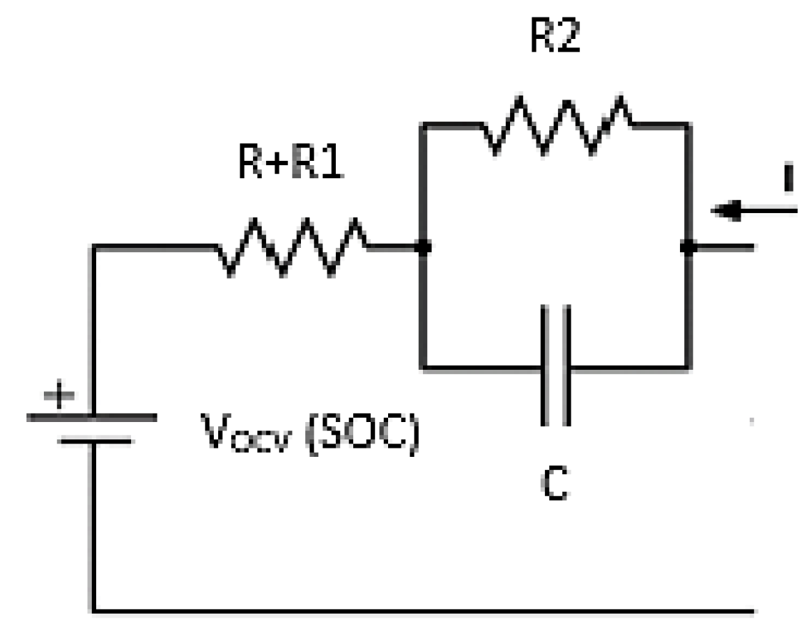
Figure 5, but in this research, a modified model is used, as can be seen in
Figure 6. Refer to
Figure 5 for a simple RC model, but this model does not replicate the actual transient behaviors of the battery and cannot accurately estimate the SOC during dynamic conditions. In order to incorporate major internal phenomena happening inside the battery during all operating conditions while keeping the circuit simple, another RC network is added. The two RC branch model simulates both the charge transfer and diffusion phenomena.
In the modified model, a parallel RC network is added to estimate the actual SOC describing the transient response of the battery during the charging and discharging phase. By the analysis of the fast Fourier transform (FFT) of the driving profile, it can be seen that most of the signal information is in the lower frequency range, and from the analysis, it can be noted that the charge transfer phenomena occur at medium frequencies [
24,
25]. The addition of the network simulates the charge transfer behaviors. Referring to
Figure 6, the resistance R1 is the charge transfer resistance and the capacitance C1 is the double layer capacitance, which will replicate the behavior during the short time constant of step response and time behavior of the terminal voltage at the depth of discharge (DOD).
From the simulation point of view, we will only consider model 2. The behavior of models 1 and 2, respectively, is different during the simulation as we have added charge transfer resistance. Model 1 simulates the ohmic and charge transfer phenomena while model 2 simulates the ohmic and diffusion phenomena. The simple RC model represents battery behavior while ignoring some parameters. Many researchers have implemented simple and modified models while varying the Warburg element [
26,
27] and can easily be found in the literature. The impedance spectra of model 1 and 2 can be seen from
Figure 7. In the next section, both of these models are validated and compared.
6.2. Validation of the Model
The model of the battery must be accurate enough to replicate the actual behavior during all operating conditions. For the verification of the battery model, validation of the model is essential. For the validation, data fitting is performed through the curve-fitting tool of MATLAB and compared with the fitted output voltage and measured voltage. Here, only the best-fit results are shown for model 1 and model 2.
Model 1: R = 0.000498, R1 = 0.000501, C1 = 171
Model 2: R + R1 = 0.000897, R2 = 0.001152, C2 = 4823561
Figure 8 in the next section shows the fitted voltage plotted with the measured voltage from the test data for models 1 and 2.
In order to check the performance of these models, the mean square error (MSE) is calculated. The MSE of model 1 is 1.15 × 10⁻², while for model 2 it is 3.02 × 10⁻³. Model 2 has less error compared to model 1 having better performance.
Figure 8 shows the fitted voltage plotted with measured voltage from the test data for models 1 and 2.
6.3. State Space Model
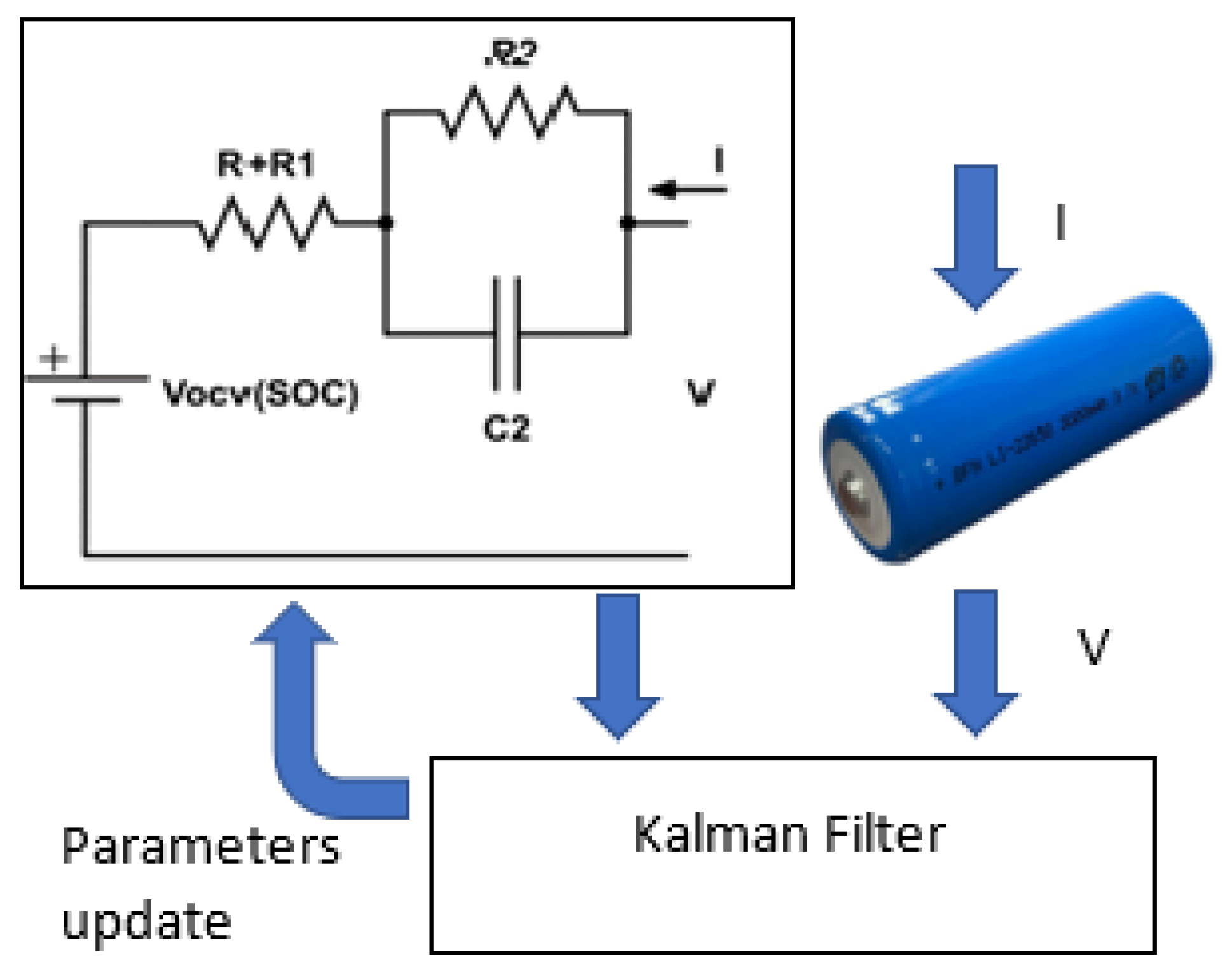
For the implementation of the Kalman filter, the state space model is developed. The general scheme for the estimation with the Kalman filter is shown in
Figure 9.
The SOC and V
R1C1 are the states to be estimated while I is the input current and V is the terminal voltage. The state vector of the system is represented as:
Assume that the cell is fully charged at time
t = 0 and the charge extracted from the cell can be defined as:
The behavior of the model in discrete time can be expressed as:
The order of the state space model is 2, so the model can be expressed in a discrete-time form using Equations (10) and (11):
and the output equation is:
where
Δt is the interval of the sample
η is the Coulombs efficiency
V_R1C1 is the voltage across the RC network
Noise is the zero mean Gaussian
For the estimation of the SOC, many authors have used the standard equation of SOC [
28,
29]. The state space representation is not unique because the authors are using different battery models or different voltage representations compared to what we are using in this paper.
The state and parameters are estimated collectively by using joint estimation while combining them to make an augmented matrix. The augmented state vector can be defined as:
where
θ is the parameter vector
Xh is the state vector
The parameters
R,
R1, and
C1 are to be estimated for model 1 and
R +
R1,
R2, and
C2 for model 2, respectively.
The state vector can be re-written as:
For joint estimation of model 1, the state space discrete form can be expressed as:
and the output equation is:
In the same way, the state space model can be developed for model 2 where the SOC, VR1 C1(k), and R, R1, R2, and C2 are the parameters to be estimated. The open circuit voltage VOCV will be found from the open circuit voltage test and simulated from a lookup table.
7. Battery Testing
For the validation of battery models, the testing of the battery is important. The SOC of the battery is related to the open circuit voltage (OCV) and by the variation in SOC; the OCV also varies but is not applicable for all lithium chemistries. The OCV of the battery cannot be measured during operation in dynamic scenarios and resting of the battery is important. For the simulation of the OCV at different SOC, a lookup table has been utilized.
7.1. Open Circuit Voltage (OCV) Testing
For the testing of the OCV, the cell was exposed at a fixed temperature of 20 °C at different SOC through the temperature chamber. A 40 Ah Kokam LiNMC cell was used for testing. For the OCV measurement, the cell was fully charged initially at 100% SOC, which further discharged at a C-rate of 0.5 to almost 0% of SOC. The discharging of the cell was stopped after every 10% of SOC, having a rest period of almost 3 h.
The same procedure was applied for the charging of the cell from 0% to 100% of the SOC with the same step and delay.
From
Figure 10, we can see voltage, current, and SOC conditions for OCV testing. During the charging and discharging, the cell remains at rest period for a sufficient amount of time so that the cells achieve equilibrium voltage. During charging and discharging phenomena, the OCV may differ because of the hysteresis effect, which is more evident in LiFeP0
4 cells and negligible in NMC lithium cells. The OCV values with respect to the SOC are mentioned in
Table 1.
7.2. Capacity Testing
To find the initial capacity of the cell, capacity testing was performed. The cell was first discharged to 0% SOC and then charged again at the same C-rate. The test was performed for three full charges and discharges and the values of capacity were noted, as can be seen from
Figure 11.
8. Simulation Results
The battery model developed in the previous section will be implemented using MATLAB. For the validation of results, a real driving profile for a 40 Ah battery having a terminal voltage of 4.2 V is utilized. The battery is fully charged to 100% of SOC initially and discharged to about 34% and then again charged to 100% of the SOC. The current and voltage profiles of the real driving profiles are shown in
Figure 12.
From the figure, we can see that the battery is discharged from 100 to almost 66% of SOC. In order to replicate the actual scenario, a rest period of about 5 h is provided. During the rest period, the battery gains capacity as the reversible resistance decreases. The battery is again discharged from 66% to 36% and charged again to 100% of SOC. A real scenario that the battery faced during operation will be depicted.
During the rest period, the irreversible resistance decreases as the temperature of the battery reduces, which is called the recuperation phenomenon. During the operating scenario, a battery may face charging, discharging, and a rest period so the real driving profile depicts this scenario.
The driving profile test was performed at the Institute of Electronics and Electrical Drives (ISEA), RWTH Aachen University, Germany. We are comparing different battery models and Kalman filters with the real driving profile in order to have a comparison about accuracy and robustness.
Model 1 and model 2 are simulated for all filters in order to compare and check the performance of different Kalman filters. The initial values of all the filters are the same. The initial state, covariance, process, and observation noise of both model 1 and 2 for the EKF and SPKF is mentioned in
Table 2 and
Table 3.
Figure 13 shows the comparison results of the SOC estimation of different Kalman filters for model 2. We have simulated both models, but the detailed result of model 2 is shown here. For model 1, only the mean square of the SOC and voltage is shown in
Table 4.
From
Figure 13, we can see that all the filters converge to the actual SOC except the EKF.
Figure 12 shows the results of the SOC estimation along with the terminal voltage plotted against the actual and estimated values. Along with the consideration of the mean square error, we are also considering another important factor which is computational complexity.
Table 5 summarizes the computational complexity along with the MSE for our main model 2. For the evaluation of the filter’s performance, we will only consider and discuss model 2.
The UKF and square root version (SRUKF) has 96.46% of SOC error improvements from the EKF. The CDKF and square root version (SRCDKF) has 96.44% error improvements. By comparing the UKF with the square root version and the CDKF with square root version, we can see that the UKF along with square root version has less estimation error, but difference is negligible. By considering computational complexity, we can see that the EFK is computationally better than the sigma point version. On the other hand, the UKF is computationally better than its square root version. In the square root version of the UKF, the Cholesky factors needs to update in the posterior. Similarly, the same will be applicable to the square root version of the CDKF.
By summarizing the above discussion, the CDKF along with the square root version is computationally less expensive compared to the UKF and square root version and the reason is because of the difference in the approximation of the posterior covariance terms. On the other hand, the CDKF and square root version uses the propagated sigma points instead of the posterior mean approximation. By comparing all the filters, we can see that the CDKF along with the square root version is the optimal choice in terms of computational complexity compared to the UKF and square root version with the same accuracy.
Figure 14 represents the comparison of the SOC estimated error for all evaluated filters. A tolerance band of 1.5% error is highlighted in the figure. We can see from
Figure 14 and
Table 2 that the EKF has more % error compared to other filters while having less computational complexity.
9. Conclusions
The EKF and UKF are derived and applied to estimate the SOC along with two different battery models (standard model as model 1 and modified model as model 2) and the results are verified with different versions of Kalman filters. We have concluded that model 2 has a better state and output compared to model 1. The possibility of joint estimation could improve the results of estimation but the accuracy of the parameters is not guaranteed because in this scenario no physical model existed.
For the verification of models and to check the performance of the filters, we compared all the filters with the MSE and computational complexity time. From the discussion in
Section 8, we concluded that the CDKF along with the square root version is better compared to the other Kalman filter versions because of having less computational complexity and the same accuracy as the UKF and square root versions. Summarizing the above discussion, the CDKF is the better choice among all other KF versions.
Author Contributions
Conceptualization, A.K. and S.A.R.K.; methodology, A.K. and M.A.; software, A.K.; validation, A.K.; formal analysis, A.K. and S.A.R.K.; investigation, A.K.; resources, M.A.; data curation, M.A.; writing—original draft preparation, A.K.; writing—review and editing, M.A.S. and N.U.A.; visualization, M.A.S. and N.U.A.; supervision, S.A.R.K.; project administration, S.A.R.K., M.A.S., J.E.M.C., J.C.V., J.M.G. and B.K. All authors have read and agreed to the published version of the manuscript.
Funding
This research received no external funding.
Data Availability Statement
The dataset used for the validation is the property of Electrochemical Energy Conversion and Storage Systems (ISEA), RWTH University Aachen, Germany.
Acknowledgments
I would like to thank Dirk Uwe Sauer, ISEA, RWTH University Aachen, Germany, of the “Electrochemical Energy Conversion and Storage Systems” (ISEA), RWTH University Aachen, Germany, for allowing the use of their research lab facilities and providing datasets for further analysis.
Conflicts of Interest
The authors declare no conflict of interest.
References
- El Kharbachi, A.; Zavorotynska, O.; Latroche, M.; Cuevas, F.; Yartys, V.; Fichtner, M. Exploits, Advances and Challenges Benefiting beyond Li-Ion Battery Technologies. J. Alloys Compd. 2020, 817, 153261. [Google Scholar] [CrossRef]
- Khalid, A.; Kashif, S.A.R.; Ain, N.U.; Nasir, A. State of Health Estimation of LiFePO4 Batteries for Battery Management systems. Comput. Mater. Contin. 2022, 73, 3149–3164. [Google Scholar] [CrossRef]
- Atalay, S.; Sheikh, M.; Mariani, A.; Merla, Y.; Bower, E.; Widanage, W.D. Theory of Battery Ageing in a Lithium-Ion Battery: Capacity Fade, Nonlinear Ageing and Lifetime Prediction. J. Power Sources 2020, 478, 229026. [Google Scholar] [CrossRef]
- Meng, J.; Yue, M.; Diallo, D. Nonlinear Extension of Battery Constrained Predictive Charging Control with Transmission of Jacobian Matrix. Int. J. Electr. Power Energy Syst. 2023, 146, 108762. [Google Scholar] [CrossRef]
- How, D.N.T.; Hannan, M.A.; Hossain Lipu, M.S.; Ker, P.J. State of Charge Estimation for Lithium-Ion Batteries Using Model-Based and Data-Driven Methods: A Review. IEEE Access 2019, 7, 136116–136136. [Google Scholar] [CrossRef]
- Kuchly, J.; Goussian, A.; Merveillaut, M.; Baghdadi, I.; Franger, S.; Nelson-Gruel, D.; Nouillant, C.; Chamaillard, Y. Li-Ion Battery SOC Estimation Method Using a Neural Network Trained with Data Generated by a P2D Model. IFAC-PapersOnLine 2021, 54, 336–343. [Google Scholar] [CrossRef]
- Zheng, W.; Xia, B.; Wang, W.; Lai, Y.; Wang, M.; Wang, H. State of Charge Estimation for Power Lithium-Ion Battery Using a Fuzzy Logic Sliding Mode Observer. Energies 2019, 12, 2491. [Google Scholar] [CrossRef]
- Zhang, Z.; Zhang, X.; He, Z.; Zhu, C.; Song, W.; Gao, M.; Song, Y. State of Charge Estimation for Lithium-Ion Batteries Using Simple Recurrent Units and Unscented Kalman Filter. Front. Energy Res. 2022, 10. [Google Scholar] [CrossRef]
- Cui, Z.; Hu, W.; Zhang, G.; Zhang, Z.; Chen, Z. An Extended Kalman Filter Based SOC Estimation Method for Li-Ion Battery. Energy Rep. 2022, 8, 81–87. [Google Scholar] [CrossRef]
- Lv, J.; Jiang, B.; Wang, X.; Liu, Y.; Fu, Y. Estimation of the State of Charge of Lithium Batteries Based on Adaptive Unscented Kalman Filter Algorithm. Electronics 2020, 9, 1425. [Google Scholar] [CrossRef]
- Zhang, Q.; Wang, D.; Yang, B.; Cui, X.; Li, X. Electrochemical Model of Lithium-Ion Battery for Wide Frequency Range Applications. Electrochim. Acta 2020, 343, 136094. [Google Scholar] [CrossRef]
- Singh, P.; Chen, C.; Tan, C.M.; Huang, S.-C. Semi-Empirical Capacity Fading Model for SOH Estimation of Li-Ion Batteries. Appl. Sci. 2019, 9, 3012. [Google Scholar] [CrossRef]
- Tran, M.-K.; Mathew, M.; Janhunen, S.; Panchal, S.; Raahemifar, K.; Fraser, R.; Fowler, M. A Comprehensive Equivalent Circuit Model for Lithium-Ion Batteries, Incorporating the Effects of State of Health, State of Charge, and Temperature on Model Parameters. J. Energy Storage 2021, 43, 103252. [Google Scholar] [CrossRef]
- Yang, S.; Zhou, S.; Hua, Y.; Zhou, X.; Liu, X.; Pan, Y.; Ling, H.; Wu, B. A Parameter Adaptive Method for State of Charge Estimation of Lithium-Ion Batteries with an Improved Extended Kalman Filter. Sci. Rep. 2021, 11, 5805. [Google Scholar] [CrossRef]
- Cui, Z.; Kang, L.; Li, L.; Wang, L.; Wang, K. A Combined State-of-Charge Estimation Method for Lithium-Ion Battery Using an Improved BGRU Network and UKF. Energy 2022, 259, 124933. [Google Scholar] [CrossRef]
- Lei, Y.; Li, R.; Yu, J.; Liu, J.; Zhang, Y.; Liu, F. Research of CDKF Based on Spectral Decomposition of Symmetric Matrix in SOC Estimation of Lithium-Ion Cell. In Proceedings of the 2021 3rd Asia Energy and Electrical Engineering Symposium (AEEES), Chengdu, China, 26–29 March 2021. [Google Scholar] [CrossRef]
- He, L.; Wang, Y.; Wei, Y.; Wang, M.; Hu, X.; Shi, Q. An Adaptive Central Difference Kalman Filter Approach for State of Charge Estimation by Fractional Order Model of Lithium-Ion Battery. Energy 2022, 244, 122627. [Google Scholar] [CrossRef]
- Ouyang, Q.; Ma, R.; Wu, Z.; Xu, G.; Wang, Z. Adaptive Square-Root Unscented Kalman Filter-Based State-of-Charge Estimation for Lithium-Ion Batteries with Model Parameter Online Identification. Energies 2020, 13, 4968. [Google Scholar] [CrossRef]
- Electrochemical Impedance Spectroscopy for Fuel Cell Research. Available online: http://www.scribner.com/wp-content/uploads/2017/06/Scribner-Associates-Electrochemical-Impedance-Spectroscopy-for-Fuel-Cell-Research.pdf (accessed on 18 December 2022).
- Rahmoun, A.; Biechl, H.; Rosin, A. SOC Estimation for Li-Ion Batteries Based on Equivalent Circuit Diagrams and the Application of a Kalman Filter. In Proceedings of the 2012 Electric Power Quality and Supply Reliability, Tartu, Estonia, 11–13 June 2012. [Google Scholar] [CrossRef]
- Tran, M.-K.; DaCosta, A.; Mevawalla, A.; Panchal, S.; Fowler, M. Comparative Study of Equivalent Circuit Models Performance in Four Common Lithium-Ion Batteries: LFP, NMC, LMO, NCA. Batteries 2021, 7, 51. [Google Scholar] [CrossRef]
- Kurzweil, P.; Scheuerpflug, W. State-of-Charge Monitoring and Battery Diagnosis of Different Lithium Ion Chemistries Using Impedance Spectroscopy. Batteries 2021, 7, 17. [Google Scholar] [CrossRef]
- Hu, L.; Hu, R.; Ma, Z.; Jiang, W. State of Charge Estimation and Evaluation of Lithium Battery Using Kalman Filter Algorithms. Materials 2022, 15, 8744. [Google Scholar] [CrossRef]
- Xu, C.; Zhang, E.; Jiang, K.; Wang, K. Dual Fuzzy-Based Adaptive Extended Kalman Filter for State of Charge Estimation of Liquid Metal Battery. Appl. Energy 2022, 327, 120091. [Google Scholar] [CrossRef]
- Xing, L.; Ling, L.; Gong, B.; Zhang, M. State-of-Charge Estimation for Lithium-Ion Batteries Using Kalman Filters Based on Fractional-Order Models. Connect. Sci. 2021, 34, 162–184. [Google Scholar] [CrossRef]
- Li, J. Adaptive Exponentially Weighted Extended Kalman Filtering for State of Charge Estimation of Lithium-Ion Battery. Int. J. Electrochem. Sci. 2022. [Google Scholar] [CrossRef]
- Hoekstra, F.; Bergveld, H.; Donkers, M. Towards State-of-Charge Estimation for Battery Packs: Reducing Computational Complexity by Optimising Model Sampling Time and Update Frequency of the Extended Kalman Filter. In Proceedings of the 2021 American Control Conference (ACC), New Orleans, LA, USA, 25–28 May 2021. [Google Scholar] [CrossRef]
- Yang, B.; Li, G.; Tang, W.; Li, H. Research on Optimized SOC Estimation Algorithm Based on Extended Kalman Filter. Front. Energy Res. 2022, 10. [Google Scholar] [CrossRef]
- Wang, Y.; Cheng, Y.; Xiong, Y.; Yan, Q. Estimation of Battery Open-Circuit Voltage and State of Charge Based on Dynamic Matrix Control-Extended Kalman Filter Algorithm. J. Energy Storage 2022, 52, 104860. [Google Scholar] [CrossRef]
| Disclaimer/Publisher’s Note: The statements, opinions and data contained in all publications are solely those of the individual author(s) and contributor(s) and not of MDPI and/or the editor(s). MDPI and/or the editor(s) disclaim responsibility for any injury to people or property resulting from any ideas, methods, instructions or products referred to in the content. |
© 2023 by the authors. Licensee MDPI, Basel, Switzerland. This article is an open access article distributed under the terms and conditions of the Creative Commons Attribution (CC BY) license (https://creativecommons.org/licenses/by/4.0/).


 ,
, 


