The Ethanol Market and Its Relation to the Price of Agricultural Commodities

Abstract

In this article, we seek to present the synthesis of the global ethanol market in the United States (US) and Brazil by using caloric equivalence to empirically characterize the elasticity of supply and demand. We also seek to evaluate the relationship between world ethanol production and prices of agricultural commodities (wheat, rice, corn, soybeans and sugar) from 1981 to 2016 using climate-induced yield shocks as instrumental variables. The main results for the world market indicate that the production and demand for ethanol respond elastically to changes in commodity prices. The world ethanol production has no significant relationship with food prices. However, evaluation of the ethanol market and its interaction with the agricultural commodities market confirms the hypothesis that Brazilian ethanol is weakly related to the price of food.

1. Introduction

The world scientific community has demonstrated constant concern for issues related to the environment, either the undesirable impacts that economic activities cause, given that climate change arises from the emission of greenhouse gases or because of possible changes in the world energy matrix due to the future scarcity of the fossil energy sources that form the basis of the current matrix, thus pointing to the need for renewable energy sources. Approximately 87% of the fuel consumed in the world is of fossil origin: mineral coal, oil and natural gas [1].

Although biofuels have gained strength as alternative sources of renewable energy, mainly due to their environmental benefits, it is considered necessary by Ferreira Filho and Horridge [2] to take into account that the worldwide expansion of biofuel production has caused concerns about its impact on food safety and supply due to competition for agricultural land. Researchers have linked this competition to recent increases in food prices. França and Gurgel [3] emphasize that the discussion about biofuels becomes even more heated when the issue of food security emerges. The evolution of food prices in the last ten years, mainly between 2005 and 2008, is a unanimous cause for concern, since food prices have risen dramatically around the world during this period.

In this context, fuel ethanol is the main biofuel globally. Thus, it becomes necessary to conduct further studies related to development of the ethanol market, since this has become an important topic in discussions regarding the global energy matrix. Such studies should aim to analyze how the effects of increased production are related to changes in the prices of agricultural commodities. To do so, studies should provide reasoning for the drafting of public policies that take into account not only environmental issues but also concerns with the increasing prices of food commodities, so that these commodities are more efficient in terms of supporting the production and commercialization of ethanol.

According to Cardoso and Bittencourt [4], becoming more familiar with the ethanol market as well as the parameters of its short- and long-term demands is essential for the preparation of public policies, especially those related to reducing fossil fuel consumption. However, the literature on ethanol demand is still scarce compared to that for gasoline, which is to be expected due to its importance as a substitute for gasoline outside Brazil, even in the United States, which is its main consumer. Compared with gasoline, the market share of ethanol was 9.84% in 2016, according to USDOE data [5].

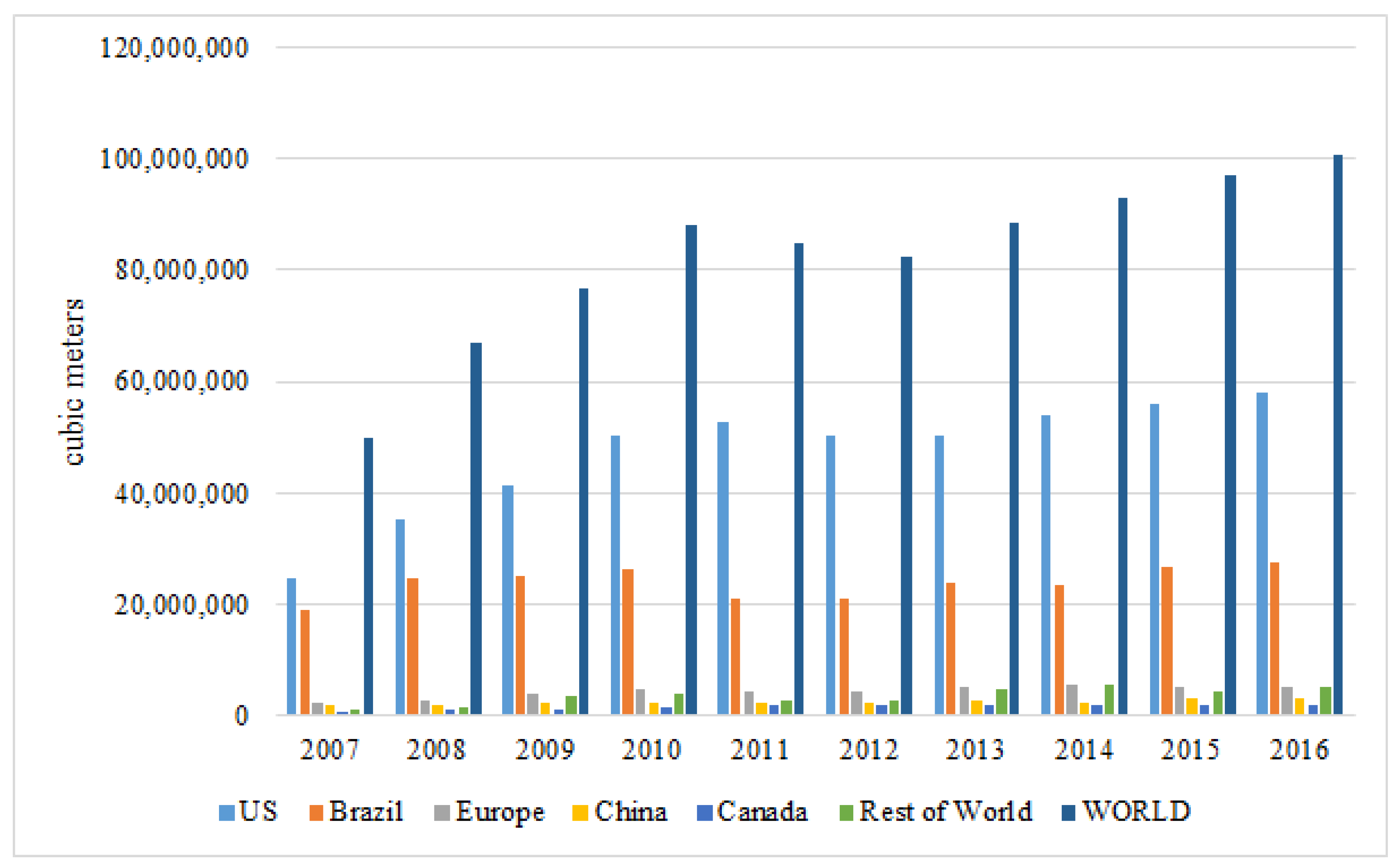
The ethanol market is led by the United States (US) and Brazil, which together account for approximately 85% of world production. According to data from the Renewable Fuels Association [6], the world production of ethanol surpassed 100 million cubic meters in 2016, equivalent to more than 100 billion liters and ethanol production in the US, at around 58 million cubic meters, represents almost 58% of world production. In that same year, Brazil accounted for around 27% of global ethanol production, with its market share reducing 10 percentage points in ten years, while the European Union accounted for just over 5% of the total volume, followed by China (3.18%) and Canada (1.64%), which were the other main producers.

The Brazilian ethanol market is one of the main ethanol markets in the world due to characteristics and specificities in terms of production and potential related mainly to the input used: sugarcane. To meet the rising demand for ethanol in other markets such as the US, large amounts of corn, soybeans, sugarcane and other plants must be used for ethanol production [7].

In this sense, Roberts and Schlenker [8] estimated the effects of the ethanol mandate in the US, suggesting that it could lead to an increase in food prices of around 30% and an increase of about 2% in the global area used for production. The price transfer occurs mainly through the use of corn as an input for ethanol production in the US and also by the substitution of other cultures for the production of corn, considering the increase in the demand for corn and the subsidies offered by the North American government. The US ethanol mandate requires that about five percent of the world’s caloric production of corn, wheat, rice and soy be used for ethanol production.

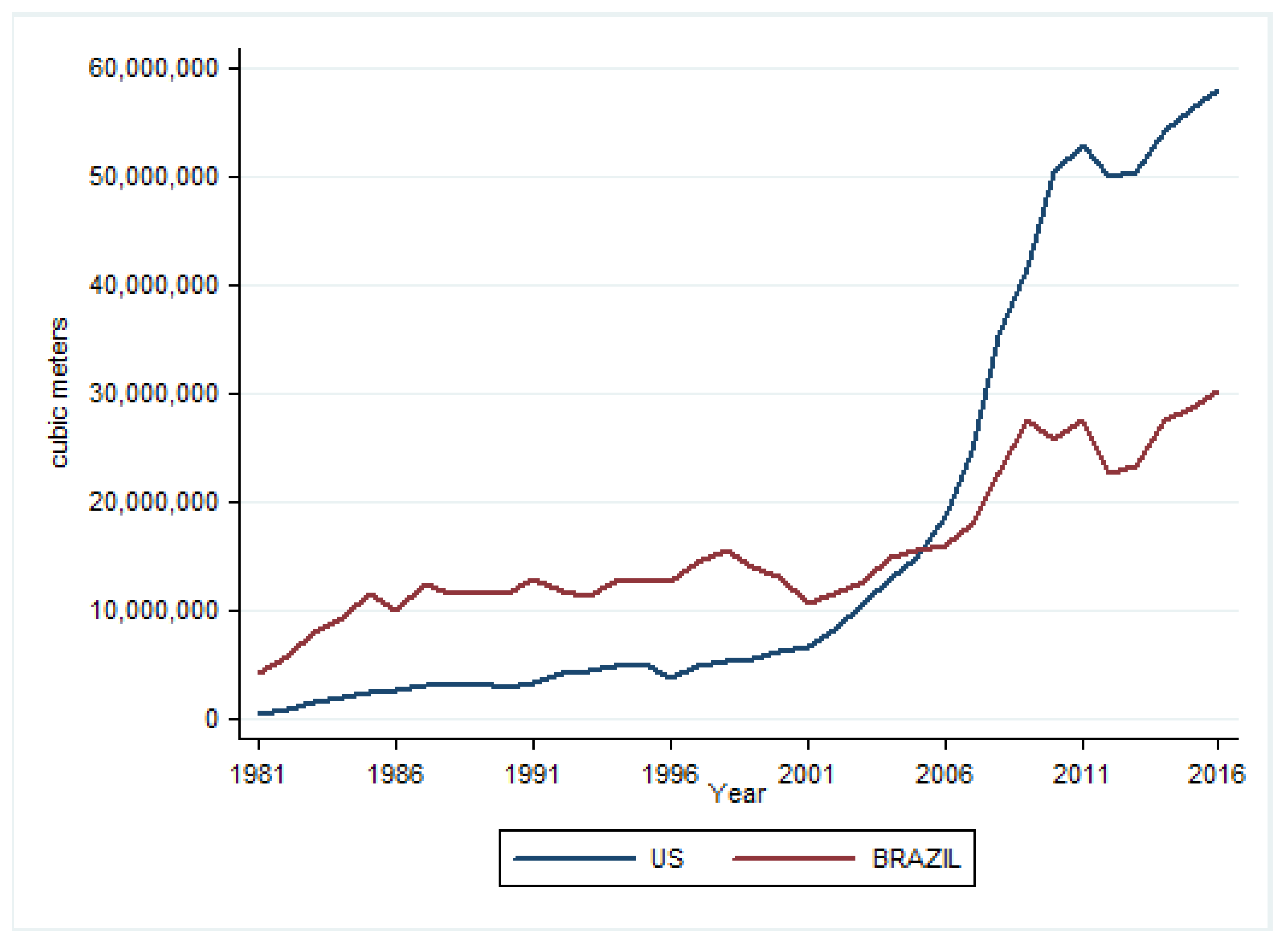
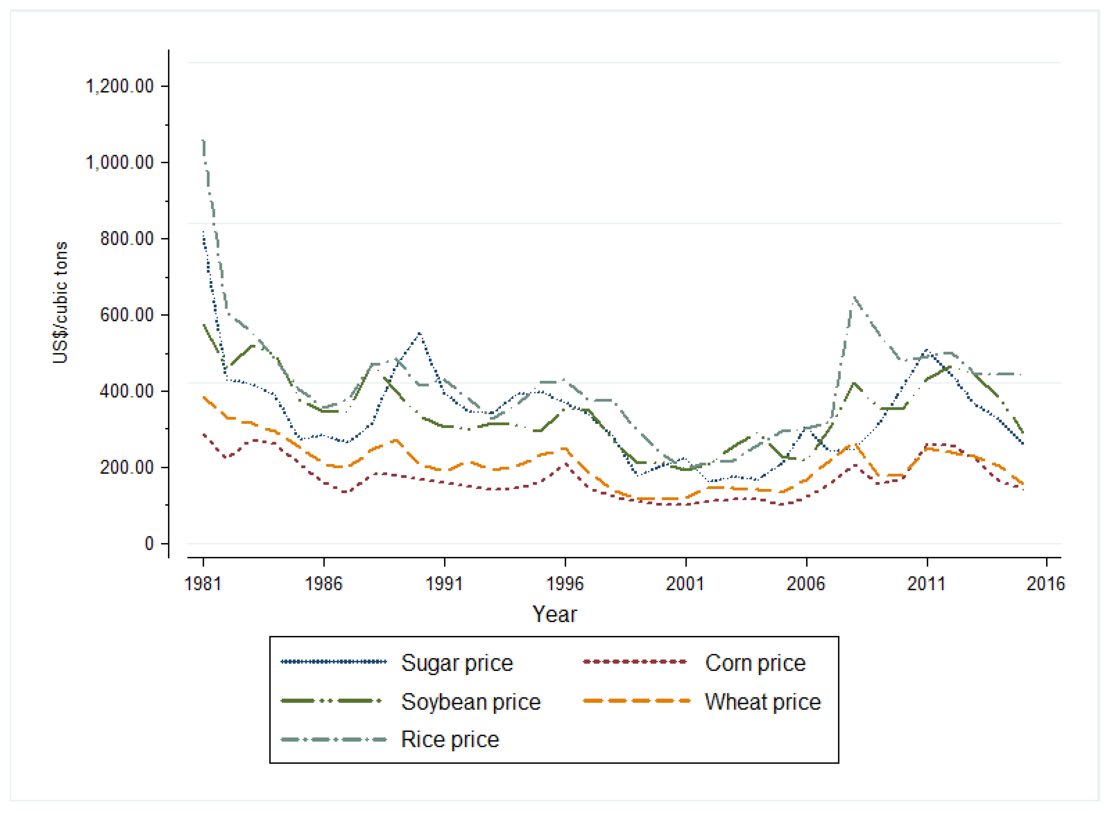
In the US, ethanol is produced from corn. In 1986, around 3.5% of corn production was destined for ethanol production and in 2016 this percentage reached just over 36% (USDOE, 2017). This shows the change in the allocation of the share produced from corn used for ethanol production. The increase in ethanol production is shown in Figure A2 and we highlight 2007 as the year in which the US became the world’s largest producer, maintaining this position until the end of the analyzed period. From 2007 onward, an upward trend in the prices of agricultural commodities can also be observed (Figure A4).

Some studies have not found evidence that the price of ethanol significantly affects the price of agricultural commodities [9,10], with others pointing out that the increased price of commodities is related to the price of oil or that it has an influence on ethanol prices [11,12]; even so, there is empirical literature relating the increase in prices, or at least part of it, to the production of biofuels [8,13,14,15,16,17]. Considering such an effect, the present study aimed to analyze the ethanol market and agricultural commodities (basic food) to identify whether or not this effect exists more broadly by considering the two main players of the ethanol market. Hence, from the results, it should be possible to point out the socially optimal result in terms of impacts and/or the interrelation of these markets in the world population.

Thus, the central point this study makes, already pointed out as a possible alternative by other studies [18], is how sugarcane-based Brazilian ethanol fits in this context either by enabling a real reduction in CO2 emissions or through benefits associated with not being directly related to the prices of the main food commodities in the world. The hypothesis that guides this study is that Brazilian ethanol may facilitate a reduction in or at least help to control the current price increases that affect the main agricultural commodities in the world (corn, wheat, rice and soy) via a reduction in the demand for corn used for ethanol production in the US.

To empirically analyze the relationship between ethanol production and the prices of agricultural commodities, this study adopted the methodology used by Roberts and Schlenker [8]. The authors presented a supply and demand model to determine the elasticity of storable commodities worldwide. The estimated elasticity is used to assess the impacts of the 2009 Renewable Fuel Standard in the US on the prices of commodities, quantities and consumer surplus.

Thus, the focus of this study was to develop a synthesis of the global ethanol market, empirically identify the elasticity of supply and demand and evaluate the relationship between world ethanol production and the prices of both the main agricultural commodities (wheat, rice, corn and soy) and also commodities linked to this sector (sugarcane).

The empirical strategy adopted here is to analyze how Brazilian and North American production are interrelated with the world market, evaluating the relationship between world production and prices. Therefore, the objective is also to estimate the supply and demand elasticity for global ethanol production based on the proposed synthesis using caloric equivalence in the analysis of interactions between the ethanol market and the main agricultural commodities.

The main results for the world market indicate that ethanol production and demand exhibit an elastic response to changes in prices. World ethanol production did not have a significant relationship with food prices, but when evaluating the ethanol market and its interaction with the agricultural commodities market, the hypothesis that Brazilian ethanol is more weakly related to food prices was verified, thus representing new empirical evidence that is the main contribution of this research.

2. Supply and Demand Model: Specification, Identification and Data

To assess the relationship between the increase in ethanol production and consumption and changes in the prices of agricultural commodities and in the income of consumers worldwide, this paper proposes a model that synthesizes the world market production using the US and Brazil in the constitution of this market, since both countries jointly represent about 85% of the world ethanol production in addition to being its main consumers, which corresponds to a representative share of the world market. In this way, it is possible to estimate the supply and demand elasticity of ethanol and its relationship with food commodities linked to this market.

To enable synthesis and interconnection with the agricultural market, this study adopted the methodology used by Roberts and Schlenker [8,19], transforming the quantities of the main worldwide commodities into food caloric equivalents using the conversion factors of Williamson and Williamson [20] and later aggregating them (quantities and prices). The agricultural products analyzed are corn, wheat, rice, soy and sugar.

The aggregation of crops facilitates the simple analysis of basic food products on a world scale. The practical reason for the aggregation is that prices of commodities tend to vary in a synchronized manner, which prevents the identification of cross price elasticity. The correlation of prices over time also suggests that the substitution possibilities are sufficiently high such that the aggregate results represent a reasonably accurate characterization of the analyzed markets [8].

2.1. Proposed Model

The analytical basis of the present study comprises studies that have analyzed the ethanol market [7,8,10,18,21,22,23,24,25,26]. The main results mostly report a positive relationship between the production of biofuels and the increase in food prices. This effect was verified mainly for the production of ethanol in the US; however, this effect has not yet been verified for Brazilian ethanol.

Thus, the proposed model seeks to synthesize the global ethanol market in order to evaluate Brazil and the US jointly and individually, verifying the relationship between ethanol production and the price of the main food commodities in the world based on the contribution of Roberts and Schlenker [8], which can be expressed in its general form as:

$$Supply:log\left(S_t\right)={\alpha }_o+{\beta }_{o}log\left(E\left[\frac{p_t}{p_{t-1}}\right]\right)+{\gamma }_o{w}_t+f\left(t\right)+u_t$$

(1)

$$Demand:log\left(D_t\right)={\alpha }_d+{\beta }_{d}log\left(p_t\right)+g\left(t\right)+X\left(t\right)+v_t$$

(2)

The quantities offered and demanded are indicated by $S_t$ and $D_t$, respectively; $p_t$ is price, which is equivalent to the marginal willingness to pay for the quantity demanded; the parameters ${\beta }_o$ and ${\beta }_d$ are the elasticity of supply and demand; $w_t$ is the yield shock induced by the climate at random; ${\alpha }_o$ and ${\alpha }_d$ are intercepts; and $f\left(t\right)$ and $g\left(t\right)$ capture temporal trends in supply and demand resulting from technological change, population growth and income growth. The variable $X\left(t\right)$ represents other country-specific variables introduced in the model. $u_t$ and $v_t$ are errors, other unobserved factors that influence supply and demand.

Given that producers make production decisions before a year-long climate shock and based on expected future prices, as well as on other supply or demand shocks that may occur, supply is linked to the expected price. Therefore, in the supply equation, the expected price (lagged in a harvest period) one year in advance is a more accurate measure of the expectations of producers.

With regard to endogeneity, Roberts and Schlenker [8] highlight that prices are key endogenous variables on the right side of supply and demand. The core of problem identification is to estimate the elasticity of supply and demand given that unobserved changes in supply and demand ($u_t$ and $v_t$) affect prices through the equilibrium identity. Without correcting price endogeneity, the elasticity of supply would be negatively biased, since unobserved positive changes in supply ($u_t$) could tend to reduce the price in a manner all the more constant, creating a negative correlation between $u_t$ and price. Likewise, the elasticity of demand would be positively biased, since unobserved positive changes in demand ($v_t$) could tend to steadily increase the price, creating a positive correlation between $v_t$ and price. If the unobserved supply and demand shifts of $u_t$ and $v_t$ are correlated, the biases may correspond to any direction.

Following the methodology adopted [8], the strategy for estimating the elasticity of supply and demand is to use the instrumental variable method (IV) by means of two-stage regression (2SLS), thus correcting endogeneity using simultaneous yield and/or lag shocks to identify demand and supply. The baseline proxy for climate-induced yield shocks are deviations from country-specific trends in the production yield of commodities linked to ethanol inputs. For this, the annual production of the analyzed commodities, specific to each country, is converted into food calories and aggregated to obtain a value for the shock to the world supply. The premise is that deviations from income trends are exogenous largely due to the random climate.

The challenges of using climate-based instruments are to obtain and link meteorological data on a worldwide scale of cultivated areas and to identify some meteorological variables strongly associated with productivity. Yield shocks are calculated as a proportion of production by country and the area dedicated to cultivating each crop as an input in ethanol production. Thus, the first stage of the regressions relates the log natural price and the log natural future prices against current and lagged yield shocks $w_t$ up to lag k. Therefore, the regressions of the first stage are:

$$log\left(p_t\right)={\pi }_{d0}+\sum _{k=0}^{k-1}{\mu }_{dk}{w}_{t-k}+{ϵ}_{dt}$$

(3)

$$log\left(E\left[p_t\right|t-1]\right)={\pi }_{s0}+\sum _{k=0}^k{\mu }_{sk}{W}_{t-k}+{ϵ}_{st}$$

(4)

At the second stage, structural Equations (1) and (2) are estimated, replacing the expected price value of the first stage for real prices. For supply Equation (1), the natural log of the production quantity is regressed in face of the forecast future price $log\left(E\widehat{\left[p_t\right|t-1]}\right)$ and the supply shifter in the current period $w_t$, plus the variable linked to the input; in the general model, the price of agricultural commodities ($P_{Al}$) is used, hereinafter called price of food. The variables excluded from the first stage to the second stage of the supply equation are the lagged yield shocks $w_{t,t}=tk-1,...,t-1$, which serve as instruments. Thus, the two-stage supply regression model can be expressed by the following equation:

$$log\left(S_t\right)={\alpha }_o+{\beta }_{o}log\left(E\left[p_t\right|t-1]\right)+{\lambda }_o{w}_t+log{P}_{Al}+u_t$$

(5)

The variable used to integrate the markets that allow for analyzing the variation in the price of food ($P_{Al}$) can be decomposed as follows:

$$P_{A{l}_t}=r_{1t}Pa{c}_{cal}+r_{2t}P{m}_{cal}+r_{3t}P{s}_{cal}+r_{4t}Pa{r}_{cal}+r_{5t}Pt{r}_{cal}$$

(6)

The price variables are price per calorie of sugar ($Pa{c}_{cal}$), price per calorie of corn ($P{m}_{cal}$), price per calorie of soy ($P{s}_{cal}$), price per calorie of rice ($Pa{r}_{cal}$) and price per calorie of wheat ($Pt{r}_{cal}$). The price of food ($P_{A{l}_t}$) is defined by the caloric portion produced (r) in the period t (${\sum }_{i=5}{r}_{it}=1$) of each commodity multiplied by their respective caloric price (USD/food calorie). In this study, quantities (kg) are transformed into food calories and their respective prices on the basis of caloric equivalence [8,19,20].

Thus, there is an average price per calorie calculated based on a diet with an average consumption of 1800 daily calories. Therefore, the variable $P_{A{l}_t}$ is the average price, in USD, spent on food for one person per year based on a daily consumption of 1800 food calories, considering the five commodities analyzed in the present study. According to the FAO [27], the average global daily consumption is 1800 calories.

In the case of demand Equation (2), the natural log of the quantity consumed is regressed in face of the predicted price, the price of a substitute good, gasoline ($P_g$) and a variable that captures the variation in income in per capita terms ($PI{B}_{pc}$). The variable excluded from the first to the second stages of the demand equation are the supply shocks $w_{t,t}=tk,...,t$. Thus, the equation that represents the regression of the estimated two-stage demand model is:

$$log\left(D_t\right)={\alpha }_d+{\beta }_d\widehat{log\left(P_t\right)}+log{P}_g+logPI{B}_{pc}+v_t$$

(7)

In addition, to estimate the ethanol supply and demand models for the US and Brazil, this study used specific variables for each country in addition to those already presented in the equations. For the US, estimates were made for the price of ethanol ($P_e$) and the price of subsidized ethanol ($P{S}_e$). The tested estimates also consider the following exogenous variables in supply Equation (5): corn price ($P_m$), corn supply ($S_m$), corn yield ($R_m$) and a variable for the portion of corn destined for ethanol production ($E{S}_m$); in demand Equation (7), these are the demand for gasoline ($D_g$), population growth ($CP$) and the market share of ethanol ($Mse$). For Brazil, the following are exogenous variables in supply Equation (5): sugar price ($P_{ac}$), sugarcane price ($P_{ca}$) and sugar supply ($S_{ac}$); in demand Equation (7), these are population growth ($CP$) and the introduction of flex-fuel vehicles tested in 2003 with the use of a dummy variable ($D2003$). The introduction of flex-fuel vehicles in 2003 made it possible for Brazilian drivers to choose between ethanol and gasoline, depending on relative prices and the fuel economy.

2.2. Identification and Method of Procedures

To identify the supply, past yield shocks (induced by climate) were used to identify the elasticity of supply ${\beta }_o$. Roberts and Schlenker [27] highlight that this is possible because past supply shocks that are induced by climate affect stocks and stocks affect the expected price in subsequent periods. The fundamental assumption for consistent identification of supply elasticity is that past supply shocks induced by the climate have zero covariance with supply shifts not observed in the current period. Unobserved supply shifts may result from recurring problems or anticipated plagues, general macroeconomic phenomena, government policies or other factors.

Therefore, the yield shock (related to climate change or temperature variation) indirectly affects production (supply), since it influences the yield of the input related to ethanol production and its final price (in the case of both sugarcane and corn), which will determine the choice of the producer in how much “effort” to devote to producing ethanol, given the price of the input (or in the case of the Brazilian producer, to direct a larger portion to sugar production).

In order to consistently identify the elasticity of demand ${\beta }_d$, it is necessary for the instrument to shift supply in a way that is plausibly unrelated to changes not observed in demand. Technically, $w_t$ should have zero covariance at $v_t$. According to the considerations of Roberts and Schlenker [27], climate is a natural instrument for three reasons: first, climate is clearly exogenous in an economic sense, as climate affects producers, but they cannot affect the climate; second, from the point of view of producers (farmers), climate is unpredictable and almost random at the time of planting, except perhaps for some cycles, such as El Niño. The randomness of the climate suggests that it is not related to broader economic conditions that are related to demand. Third, the climate has an obvious causal link in the supply of agricultural commodities, which, in general, appears to have little or no direct influence on demand. It is possible that climate may influence and change tastes, hunger or general caloric needs.

In addition, other instrumental variables were tested in the identification. Of these, the one found to be significant for model robustness and used in the caloric equivalence models is the number of people that can be fed ($H_{al}$) considering a daily diet of 1800 calories (used as a log) based on the caloric production of each country.

Thus, we progress to the identification of elasticity using shocks to specific yields of each crop induced by the climate. First, the models with variables only for the ethanol market and specific yields for each crop are individually estimated for each country (using 2SLS), as performed according to Luchansk and Monks [7] for the US and, subsequently, both individually and aggregated. The general model is estimated using food caloric equivalence to aggregate the agricultural commodities market (in relation to quantities, prices and yield) and a further model with IV panel data is used considering the 2SLS estimator to estimate the relationship between the global ethanol production market (assumed as US and Brazil in the present study) and the basic food commodities market.

2.3. Data Source

The analysis period is related to the availability of data and information by the government agencies of the US and Brazil, which are responsible for monitoring the biofuels sector and also with the Food and Agriculture Organization of the United Nations [28] and the International Monetary Fund [29]. Thus, the database consists of variables with an annual periodicity covering the period from 1981 to 2016 and the monetary values were corrected (deflated) to the dollar value (USD) in 2015. Below, this study presents a summary of some of the variables used and their sources. Presented in Figure A1 (Appendix A) is a complete characterization of all the information and the units of measurement for all categorizations.

The database consists of variables related to ethanol production and consumption, used as a proxy for supply and demand and the price of ethanol. For the US, this information was obtained from the USDOE (production and consumption) and the Nebraska Energy Office [30] (price).

For Brazil, these variables were obtained from IPEADATA [31] using ANP [32] information as the primary source. The production variables and prices of agricultural commodities, both for the US and Brazil, were the production of soy, rice, wheat, sugarcane and sugar [28]; corn production ([33] for the US and [31] for Brazil); and the price of soybeans, corn, rice, wheat and sugar ([29] internationally). Other variables are the price and consumption of gasoline ([5,30], respectively, for the US and [31,32], respectively, for Brazil) and climate change [28].

3. Results and Discussion

This section presents the results for the ethanol supply and demand models as well as for the relationship between the models and the food commodities market. The procedure adopted for estimations and the presentation of results (

Table 1. Ethanol supply and demand model for the US.

Variable	(1)	(2)	(3)	(4)	(5)	(6)
A. Supply Model
Constant	−104.91 ***	−35.04 **	−123.09 ***	−86.49 ***	−134.53 ***	−125.17 ***
	(10.2816)	(14.3803)	(22.8157)	(23.9361)	(6.7460)	(6.7681)
lnPe (t − 1)	−0.1005		1.9802		0.3519 *
	(0.2921)		(1.7909)		(0.2052)
lnPSe (t − 1)		−0.1022		1.2505		0.2850 *
		(0.1448)		(1.1375)		(0.1602)
lnPm	0.1725	−0.4973 ***	−0.8023	−0.8225
	(0.1708)	(0.1646)	(0.9086)	(0.9274)
lnOm	6.4488 ***	2.8231 ***	6.9566 ***	5.3051 ***
	(0.5705)	(0.7611)	(1.0905)	(1.4447)
lnRm	−1.90 **	−0.4722	−1.8109	−1.5199
	(0.8588)	(0.6794)	(1.3348)	(1.3494)
lnPAl					0.7426 ***	0.6470 **
					(0.1982)	(0.2136)
lnRCM					9.5530 ***	9.0033 ***
					(0.4153)	(0.5481)
ESm		0.0511 ***
		(0.0091)
IV	No	No	Yes	Yes	Yes	Yes
R-squared	0.9314	0.9696	0.7839	0.7926	0.9363	0.9343
F-stat	115.63 ***	256.52 ***
B. Demand Model
Constant	43.29	−35.48 *	87.49 **	14.43	14.17	−64.43 ***
	(32.3691)	(19.0206)	(39.8071)	(53.3604)	(29.0068)	(7.0568)
lnPe	−1.6961 ***		−4.0158 ***		−4.3397 ***
	(0.5391)		(1.1242)		(1.4529)
lnPSe		−0.1291		−0.3306		−0.4482
		(0.1379)		(1.3308)		(1.7216)
lnPg	1.6285 ***	0.2275	3.0116 ***	1.1724	3.2642 ***	1.2468*
	(0.3795)	(0.1592)	(0.6219)	(1.2756)	(0.9628)	(0.6717)
lnDg	−6.6717 **	0.2980	−6.8382 **	−7.0358 *
	(2.8155)	(1.9252)	(2.8123)	(4.0331)
lnPIBpc	9.9705 ***	4.1029 **	6.7276 **	12.7094 ***	0.8771	7.0193 ***
	(2.3909)	(1.8451)	(2.779)	(2.7034)	(2.4051)	(0.6327)
CP	−0.5381	0.0888			0.4399
	(0.4138)	(0.1877)			(0.6505)
Mse		0.1938 ***
		(0.0162)
IV	No	No	Yes	Yes	Yes	Yes
R-squared	0.9431	0.9885	0.9133	0.9138	0.8913	0.8970
F-stat	277.46 ***	497.73 ***

Note: Columns 1 to 4 represent the estimates using monetary values for prices of food commodities, while columns 5 and 6 show estimates transformed into caloric equivalents. Robust standard errors in parentheses. *** p < 0.01, ** p < 0.05, * p < 0.1. Source: Research results.

,

Table 2. Ethanol supply and demand model for Brazil.

Variable	(1)	(2)	(3)
A. Supply Model
Constant	4.4488	0.2257	3.0532
	(1.4080)	(6.8276)	(5.3243)
lnPe (t − 1)	−0.0742	3.5615 ***	3.4183 ***
	(0.2526)	(1.3354)	(1.2888)
lnPac	0.4881 ***	−0.9242 **
	(0.1572)	(0.3915)
lnPca	−0.1903 *	−0.6410
	(0.1070)	(0.4406)
lnOac	0.6119 ***
	(0.0986)
lnPal			−1.6429 *
			(0.8956)
IV	No	Yes	Yes
R-squared	0.7482	0.6125	0.6589
F-stat	30.55 ***
B. Demand Model
Constant	12.6883	−14.0902	−8.4724
	(13.8388)	(103.0853)	(92.0453)
lnPe	1.0947 **	−0.8548	−0.3124
	(0.4830)	(7.1341)	(5.6588)
lnPg	−1.3076 **	0.2683	−0.2357
	(0.5239)	(5.6053)	(4.0437)
lnPIBpc	0.6795	3.595	2.9979
	(1.4141)	(11.2865)	(10.1718)
CP	−0.6015	0.2169	0.1473
	(0.5876)	(3.2291)	(3.4235)
D2003	0.0536	−0.1549
	(0.2681)	(0.776)
IV	No	Yes	Yes
R-squared	0.7588	0.6403	0.6953
F-stat	21.37 ***

Note: Columns 1 and 2 represent the estimates using monetary values for prices of food commodities, while column 3 shows estimates transformed into caloric equivalents. Robust standard errors in parentheses. *** p < 0.01, ** p < 0.05, * p < 0.1. Source: Research results.

and

Table 3. Ethanol supply and demand model for the world ethanol market.

Variable	(1)	(2)	(Variable)	(3)	(4)
A. Supply Model			B. Demand Model
Constant	14.9651 ***	9.5901 *	Constant	4.4124	11.6160 ***
	(2.8355)	(5.4763)		(2.8466)	(4.0456)
lnPe (t − 1)	−0.4324	1.3464 *	lnPe	−2.8832 ***	−5.3518 ***
	(1.0439)	(0.7899)		(0.9438)	(0.8453)
lnPal	0.7523	−0.3575	lnPg	2.6531 ***	3.6461 ***
	(0.6906)	(0.1102)		(0.3848)	(0.4044)
IV	No	Yes	lnPIBpc	1.3054 ***	1.5425 ***
Observations	69	69		(0.0729)	(0.2114)
			VI	No	Yes
			Observations	71	71

Note: Robust standard errors in parentheses. *** p < 0.01, * p < 0.1. Source: Research results.

) consisted of initially analyzing the ethanol market in the US and Brazil separately, estimating (2SLS) the supply and demand equations of ethanol in the respective markets using the base input price (monetary values for quantity). In the analysis of the relationship with the agricultural market, the procedure considered the price according to caloric equivalence (monetary value per calorie). After individually analyzing the markets considering their specifications and caloric equivalence, a panel data model containing the 2SLS estimator was used by applying the Baltagi [34] estimator (EC2SLS) to assess the market in an aggregate manner.

Table 1 shows the results for the US ethanol market. At first, models were estimated using ordinary least squares (columns 1 and 2) and, later, the instrumental variables estimator (columns 3 to 6).

As Table 1 shows, the elasticity price coefficients of supply in non-instrumented models (panel A) are not statistically significant and present a sign contrary to the theory (indicating a negative trend in supply elasticity when the estimation does not consider endogeneity) in addition to being highly inelastic. However, by instrumenting the model, the price elasticity of supply becomes positive, indicating that increases in the price of ethanol ($P_e$ and $P{S}_e$) have a positive effect on its supply (models in columns 3 to 6). However, it becomes statistically significant only when considering caloric equivalence (columns 5 and 6). Thus, the supply response to price changes is elastic (1.98 and 1.25 for columns 3 and 4, respectively) for the model without caloric equivalence and inelastic (0.49 and 0.48 for columns 5 and 6, respectively) for the caloric equivalence models.

Therefore, increases in the price of ethanol lead to positive variation in the ethanol supply, which is in accordance with the theory and with the results found by Luchansky and Monks [7]. The supply price elasticity for the US is estimated considering the price of ethanol paid to the producer and the subsidized price of ethanol ($P_e$ and $P{S}_e$, respectively), which results from government subsidies that are discounted in the final composition of the price.

Regarding the ethanol supply model, the positive and statistically significant relationship with the price of food (0.74 and 0.65), that is, increases in equivalent food prices ($P_{Al}$) by 1%, leads to an increase in the supply of ethanol of approximately 0.74% (column 5, panel A) when keeping the other variables constant. This shows a strong positive relationship (they are positively correlated) with the prices of the other commodities under analysis, since for the price of corn, the main input of American ethanol, prices have a negative relationship with the supply of ethanol (−0.80 and −0.82, columns 3 and 4, respectively), even if they have no statistical significance, which makes the analysis limited in terms of these coefficients. However, they are in accordance with the economic theory and with the results reported by Luchansky and Monks [7] for the price of corn ($P_m$) in the US.

With respect to the variable food prices ($P_{Al}$), there is a positive effect in relation to the increase in ethanol production; that is, there is a significant relationship between increasing food prices in the US and the expansion of North American ethanol supply.

As for the ethanol demand model for the US (Table 1), as the demand is instrumentalized, the elasticity of demand becomes more elastic and negatively related (according to the theory) to the demand for ethanol and this is significant (with the exception of the model in column 6, which considers subsidized prices). This result was also observed by Luchansk and Monks [7] upon analyzing the ethanol market in the US. The price elasticity of demand of −4.34 indicates that a 1% increase in the price of ethanol leads to a 4.34% decrease in the demand for ethanol, ceteris paribus. Therefore, the magnitude of the response to price changes is greater on the demand side.

There is a positive and statistically significant relationship between gasoline cross price elasticity in relation to ethanol demand, in addition to being elastic in both models (3.01 and 3.26 for models without and with caloric equivalence, respectively, considering the model of non-subsidized prices), showing that it is an adequate substitute in the North American market. Therefore, increases in the price of gasoline lead to a greater demand for ethanol.

The same effect also occurs with respect to increases in per capita income, which were shown to be statistically significant in almost all models (with the exception of column 5) in explaining variations in the demand for US ethanol. When the price of ethanol with subsidies is considered in the analysis ($P{S}_e$, columns 4 and 6), the results are not statistically significant with respect to the elasticity of demand price, which was expected since these are not the prices practiced in the market. Thus, they cannot explain the variations in ethanol demand.

The results presented in Table 2 refer to the supply and demand model for the Brazilian ethanol market from 1981 to 2016. For the supply model (panel A), when the model is not instrumentalized, the price elasticity of supply ($P{e}_{t-1}$) is inelastic, negative and not significant. However, after instrumentalization, it increases in magnitude, becoming elastic (3.5615 and 3.4183) and statistically significant for both models (with and without caloric equivalence: columns 3 and 4, respectively). The effect is in accordance with the theory, since the elasticity of supply is positive. Therefore, the price elasticity of supply indicates that changes in the price of ethanol have a greater effect on the supply side, with a 1% change in the price of ethanol leading to an increase of approximately 3.4% to 3.6% in the supply of ethanol.

In the supply model (panel A, columns 1 and 2), the results for the sugar and sugarcane price coefficients showed a negative relationship with the ethanol production in Brazil, as expected. In the Brazilian market there is the possibility of sugarcane (input) being used for the production of sugar or ethanol, this decision depends on the relative price ratio between the two products. When there is a favorable price ratio for sugar in relation to ethanol, it reduces the supply of ethanol. As an example, the results show if the price of sugar increases by 1%, the supply quantity of ethanol will reduce by approximately 0.92%, ceteris paribus.

For the caloric equivalence model, the variable for food prices ($P_{Al}$) is found to be statistically significant in explaining the Brazilian ethanol supply, with a negative relationship. Therefore, the increase in the ethanol supply in the Brazilian market has a significant and negative relationship with the prices of the agricultural commodities under analysis, showing that when food prices increase by one percentage point and keeping the other variables constant, there is a reduction of 1.64% in the supply of ethanol.

Regarding the demand model (panel B, Table 2), the price elasticity of demand has a positive relationship for the non-instrumentalized model (IV). However, for the models with IV, it becomes negative, which is in accordance with the theory, since price increases reduce the demand for ethanol. However, it was not significant and inelastic (−0.8548 and −0.3124) even in the calorie equivalence model (column 4).

For the cross price elasticity of gasoline, a contradictory result is observed in the caloric equivalence model: it was negative. However, for the model without equivalence, its coefficient is positive, indicating that increases in the price of the substitute good lead to a greater demand for ethanol, as expected. However, there the price increase is relatively low, since the response is inelastic (0.2683). This partially contradictory effect may result from a good portion of the ethanol produced and consumed in the Brazilian market being used together with gasoline (as a mixture), which results in these fuels being listed as complementary.

The demand response to variations in income is elastic (2.99 and 3.59), indicating that ethanol can be considered a normal good in Brazil. Therefore, the income elasticity shows that a 1% change in the income leads to an increase of approximately 2.99% to 3.59% in the demand quantity of ethanol. However, this relationship is not statistically significant. Population growth showed a positive relationship with ethanol demand quantity, but also not significant.

Finally, the variable created to capture the change in the ethanol demand pattern after the introduction of flex-fuel (D2003) cars was not significant, indicating that there is no change in the pattern. However, the results for demand models with IV did not present a statistical significance for the considered variables, which makes their analysis limited. However, a possible explanation for this is related to the time window (annual data), which presents limitations due to the period under analysis and data availability, which does not invalidate the economic sense of the results given the series available and used in the present analysis.

Table 3 shows the results for the ethanol supply and demand model for the world market. Based on the caloric equivalence, with respect to the variables linked to the analyzed agricultural commodities, all estimated models (Table 3) use aggregation and are instrumented with caloric yield shocks induced by the specific climate of each country. The specifications and variables were presented in the previous section.

In panel A (column 2), the global ethanol supply model shows an elastic and significant response to changes in price (1.3464), which is in line with expectations, since price increases should lead to a greater quantity to be produced in the next period. The cross price elasticity with food was negative and without a statistical significance. The negative relationship of food prices ($P_{Al}$) with the supply of ethanol is to be expected given the relationship with the input of this variable. However, this variable has no statistically significant relationship for explaining the variations in the supply of ethanol. Therefore, when the market is analyzed in an aggregate way, there is no significance of this variable in explaining the ethanol supply. Differently, when the markets are individually analyzed, there is an indication of price relationship between ethanol production and food prices, though with divergent signs for the US and Brazil.

Regarding the demand model (panel b, column 4), a statistically significant, highly elastic response (−5.35) to changes in price was found, showing a negative relationship between ethanol price and demand; that is, price increases lead to a reduction in consumption (demand), as theoretically expected. Therefore, an increase in the average ethanol price of 1% is associated with a reduction in ethanol demand quantity in the world of 5.35%.

The cross price elasticity of gasoline in relation to demand presents a positive (3.65) and statistically significant relationship, showing that gasoline is an adequate substitute for ethanol in the world market. Therefore, positive price variations of gasoline lead to a greater demand for ethanol consumption in replacing gasoline. In the same way, they increase the price of ethanol while reducing the demand for ethanol, increasing the demand for gasoline, in light of the substitution effect.

The demand elasticity income coefficient ($PI{B}_{pc}$) also shows a positive sign (1.54), which is significant and greater than the unit, indicating that ethanol is a normal good for which the demand is positively affected by increases in income. For each rise of 1% in the average income, an increase of 1.54% is expected in the demand for ethanol in the world.

In summary, the results of ethanol supply and demand models show that when the ethanol market is analyzed in aggregate, ethanol production does not present a significant relationship with the price of agricultural commodities. When analysis is individually conducted for countries, such as in the case of the US, this relationship becomes significant and is positive; for Brazil, the relationship, besides being significant, is negative. This shows that positive variations in the price of food imply an increase in ethanol production in the US and, conversely, a reduction for Brazil. In this sense, increased use of Brazilian ethanol, to the detriment of US ethanol, could contribute to the existing price ratio, softening the impact on the price of food or even ceasing to be significant when the market is analyzed together.

4. Conclusions

This study aimed to estimate the supply and demand elasticity in global ethanol production based on the proposed synthesis using caloric equivalence in the analysis of interactions between the ethanol market and the main agricultural commodities.

An important growth in world production and demand for ethanol was identified for the period from 1981 to 2016, as well as a consolidation that occurred gradually in the US as the largest producer, consumer and exporter of ethanol in the world.

For the US ethanol market, ethanol production shows an inelastic relationship to price that is statistically significant when caloric equivalence is used in the analysis and the relationship is elastic and not significant when equivalence is not taken into account. A positive relationship was found in all instrumented models, indicating that changes in demand are reflected as price increases that are relatively larger than the actual changes in production (inelastic response). Although no significant relationship between corn price and ethanol production was found in the equivalence model, the production of ethanol shows a positive and significant relationship with the price of food. The price elasticity of demand indicates a strong relationship between consumption and the price of ethanol, as well as the elasticity of income. The results also indicate that gasoline is considered an adequate substitute for ethanol in the US market.

The Brazilian ethanol market showed statistically significant price elasticity in response to supply, indicating that the efforts dedicated to production are highly influenced by the predicted prices. The production (supply) of ethanol in Brazil shows a significantly negative relationship with the price of food, in contrast to that verified for production in the US. The demand is inelastic with respect to price and there is a negative, though insignificant, relationship between ethanol consumption (demand) and price. The cross price elasticity shows that gasoline is a substitute for ethanol in Brazil in the model without caloric equivalence. However, the coefficient is not statistically significant.

Among the main results for the global ethanol market, there is a statistically significant elastic response of ethanol production to changes in ethanol price. Therefore, changes in demand will mainly lead to changes in ethanol production instead of variations in the price of ethanol. Another interesting result is that world ethanol production is not statistically significantly related to food prices. On the demand side, the high price elasticity of demand suggests that ethanol prices have a strong effect on the quantity of demanded ethanol.

Therefore, regarding the study hypothesis that Brazilian ethanol may facilitate a reduction in or at least help control the price increases affecting the main agricultural commodities in the world by reducing the demand for corn for use in ethanol production in the US, it appears that this may be an alternative to possible public policies aimed at increasing use of Brazilian ethanol relative to North American ethanol; that is, larger-scale use of the Brazilian product to the detriment of the American product may have a comparatively lower impact on food price.

The contribution of this work is estimates of supply and demand elasticity at the international (worldwide) level for the ethanol market, thus representing a novel contribution not yet documented in the existing literature. Among the main results, it is worth highlighting that the results of this study demonstrate that the Brazilian product can have a possible positive influence if used on a larger scale and to the detriment of the North American product in the current scenario of rising prices of food commodities worldwide. In addition, regarding the ethanol market, there is an empirical contribution in relation to the calorie equivalence model, analyzed individually for Brazil and the US, with aggregation of the global ethanol market, which had so far been unexplored.

The results also contribute to future studies evaluating the effects of using more corn on Brazilian ethanol production, which still has a low percentage of corn use as input in ethanol production (less than 5% in 2019 [35]). This reduced percentage of corn use in Brazilian ethanol production is one of the factors that explain why the ethanol production has no relation with the increase in the Brazilian food prices. This aspect is different from the American market, where most of the input used for ethanol production is corn.

Regarding possible limitations, future studies should strive for advances in relation to the amplitude of the global ethanol market in a way not limited only to the two main consuming and producing countries. However, for this, ethanol use should be increased in these markets on a continuous basis and there must be greater monitoring in terms of statistical information in the countries that have more recently become part of the market. Another possible limitation is the aggregation of food commodities in relation to the prices and equivalent yields (caloric) of the analyzed variables. However, an “approximate” dimension of the expansion of the world market and its interaction with the agricultural commodities market is becoming necessary.

References

1. IEA. International Energy Agency. Available online: http://www.iea.org/ (accessed on 18 June 2018).
2. Ferreira Filho, J.B.S.; Horridge, M. Ethanol expansion and indirect land use change in Brazil. Land Use Policy 2014, 36, 595–604. [Google Scholar] [CrossRef] [Green Version]
3. França, A.C.; Gurgel, A.C. O efeito do Padrão de Combustíveis Renováveis Norte-Americano sobre o uso da terra no Brasil: Uma análise à luz de um modelo computável de equilíbrio geral. In 42° Encontro Nacional de Economia; SOBER: Natal, Brazil, 2014. [Google Scholar]
4. Cardoso, L.C.B.; Bittencourt, M.V.L. Mensuração das elasticidades-preço da demanda, cruzada e renda no mercado de etanol brasileiro: Um estudo usando painéis cointegrados. Rev. Econ. Sociol. Rural. 2013, 51, 765–784. [Google Scholar] [CrossRef] [Green Version]
5. USDOE. U.S. Department of Energy. Alternative Fuels Data Center. Available online: http://www.afdc.energy.gov/data/search?q=ethanol (accessed on 25 August 2017).
6. RFA. Renewable Fuels Association. Available online: http://ethanolrfa.org/ (accessed on 10 October 2017).
7. Luchansky, M.S.; Monks, J. Supply and demand elasticities in the US ethanol fuel market. Energy Econ. 2009, 31, 403–410. [Google Scholar] [CrossRef]
8. Roberts, M.J.; Schlenker, W. Identifying Supply and Demand Elasticities of Agricultural Commodities: Implications for the US Ethanol Mandate. Am. Econ. Rev. 2013, 103, 2265–2295. [Google Scholar] [CrossRef] [Green Version]
9. Zhang, Z.; Lohr, L.; Escalante, C.; Wetzstein, M. Food Versus Fuel: What Do Prices Tell Us? Energy Policy 2010, 38, 445–451. [Google Scholar] [CrossRef]
10. Bastianin, A.; Galeotti, M.; Manera, M. Ethanol and field crops: Is there a price connection? Food Policy 2016, 63, 53–61. [Google Scholar] [CrossRef]
11. Serra, T. Volatility Spillovers between Food and Energy Markets: A Semiparametric Approach. Energy Econ. 2011, 33, 1155–1164. [Google Scholar] [CrossRef] [Green Version]
12. Serra, T.; Zilberman, D.; Gil, J. Price Volatility in Ethanol Markets. Eur. Rev. Agric. Econ. 2011, 38, 259–280. [Google Scholar] [CrossRef] [Green Version]
13. Zhang, Z.; Lohr, L.; Escalante, C.E.; Wetzstein, M.E. Ethanol, Corn and Soybean Price Relations in a Volatile Vehicle-fuels Market. Energies 2009, 2, 320–339. [Google Scholar] [CrossRef] [Green Version]
14. Al-Riffai, P.; Dimaranan, B.; Laborde, D. Global Trade and Environmental Impact Study of the EU Biofuels Mandate; IFPRI: Washington, DC, USA, 2010; Volume 125. [Google Scholar]
15. Serra, T.; Zilberman, D.; Gil, J.M.; Goodwin, B.K. Nonlinearities in the US Corn-Ethanol-Oil Price System. Agric. Econ. 2011, 38, 259–280. [Google Scholar]
16. Chakravorty, U.; Hubert, M.H.; Moreaux, M.; Nostbakken, L. Will Biofuel Mandates Raise Food Prices? Working Paper No. 2011–01; University of Alberta: Edmonton, AL, Canada, 2010. [Google Scholar]
17. Kristoufek, L.; Janda, K.; Zilberman, D. Topological Properties of Biofuels Networks; Working Paper; University of Prague: Prague, Czechia, 2011. [Google Scholar]
18. Zilberman, D.; Hochman, G.; Rajagopal, D.; Sexton, S.; Timilsina, G. The impact of biofuels on commodity food prices: Assessment of findings. Am. J. Agric. Econ. 2013, 95, 275–281. [Google Scholar] [CrossRef]
19. Roberts, M.J.; Schlenker, W. World Supply and Demand of Food Commodity Calories. Am. J. Agric. Econ. 2009, 91, 1235–1242. [Google Scholar] [CrossRef]
20. Williamson, L.; Williamson, P. What We Eat. J. Farm Econ. 1942, 24, 698–703. [Google Scholar] [CrossRef]
21. Gardner, B. Fuel ethanol subsidies and farm price support. J. Agric. Food Ind. Organ. 2007, 5, 4. [Google Scholar] [CrossRef]
22. Chagas, A.L.S.; Toneto-Júnior, R.; Azzoni, C.R. Teremos que trocar energia por comida? Análise do impacto da expansão da produção de cana-de-açúcar sobre o preço da terra e dos alimentos. In Proceedings of the 46th Congress, Rio Branco, Brazil, 20–23 July 2008. [Google Scholar]
23. Searchinger, T.; Heimlich, R.; Houghton, R.A.; Dong, F.; Elobeid, A.; Fabiosa, J.; Tokgoz, S.; Hayes, D.; Yu, T.H. Use of US croplands for biofuels increases greenhouse gases through emissions from land-use change. Science 2008, 319, 1238–1240. [Google Scholar] [CrossRef] [PubMed]
24. Pacini, H.; Silveira, S. Consumer choice between ethanol and gasoline: Lessons from Brazil and Sweden. Energy Policy 2011, 39, 6936–6942. [Google Scholar] [CrossRef]
25. Anderson, S.T. The demand for ethanol as a gasoline substitute. J. Environ. Econ. Manag. 2012, 63, 151–168. [Google Scholar] [CrossRef] [Green Version]
26. Timilsina, G.R.; Beghin, J.C.; Van Der Mensbrugghe, D.; Mevel, S. The impacts of biofuels targets on land-use change and food supply: A global CGE assessment. Agric. Econ. 2012, 43, 315–332. [Google Scholar] [CrossRef] [Green Version]
27. FAO. Food and Agriculture Organization of the United Nations. Available online: http://www.fao.org/home/en/ (accessed on 7 September 2017).
28. FAOSTAT. Food and Agriculture Organization of the United Nations, Statistics. Available online: http://faostat3.fao.org/home/E (accessed on 28 June 2017).
29. IMF-IFS. International Monetary Fund, International Financial Statistics. Available online: http://www.imf.org/en/Data (accessed on 7 September 2017).
30. NEO. Nebraska Energy Office. Available online: http://www.neo.ne.gov (accessed on 10 October 2017).
31. IPEADATA. Instituto de Pesquisa Econômica Aplicada. Available online: http://www.ipeadata.gov.br (accessed on 10 October 2017).
32. ANP. Agência Nacional do Petróleo, Gás Natural e Biocombustíveis. Available online: http://www.anp.gov.br/ (accessed on 20 October 2017).
33. USDA. United States Department of Agriculture. Available online: https://www.nass.usda.gov/QuickStats/ (accessed on 10 October 2017).
34. Baltagi, B.H.; Liu, L. A note on the application of EC2SLS and EC3SLS estimators in panel data models. Stat. Probab. Lett. 2009, 79, 2189–2192. [Google Scholar] [CrossRef] [Green Version]
35. CONAB. Companhia Nacional de Abastecimento. Available online: http://www.conab.gov.br/ (accessed on 24 January 2023).