Article

Investigating the Spatial Spillover Effect of Transportation Infrastructure on Green Total Factor Productivity

1
School of Finance and Economics, Jiangsu University, Zhenjiang 212013, China
2
School of Automotive and Traffic Engineering, Jiangsu University, Zhenjiang 212013, China
3
Department of Business Administration, Sukkur IBA University, Sukkur 65200, Pakistan
*
Author to whom correspondence should be addressed.
Energies 2023, 16(6), 2733; https://doi.org/10.3390/en16062733
Submission received: 24 January 2023 / Revised: 27 February 2023 / Accepted: 9 March 2023 / Published: 15 March 2023

Abstract

:
Green development and the high-quality economic growth model have replaced the extensive growth model in an effort to reduce the large amounts of energy consumption and pollution emissions. Green total factor productivity has become an important indicator to more accurately measure the quality of economic growth. Transportation infrastructure is a fundamental component that may effectively integrate regional resources, increase regional cooperation, and encourage the sensible use of resources, and is a key factor in increasing productivity. At present, transportation infrastructure should focus on the speed of construction and the quality level, expand the radiation range of the transportation system, improve the service level of transportation facilities, and promote the spatial coordination between transportation facilities and resources and the environment in each province. Therefore, it is of great significance to study the spatial effect of the transport infrastructure on green total factor productivity in order to understand the role of transport infrastructure and its impact on the quality of economic growth. In this study, the slacks-based measure (SBM) model and the global Malmquist–Luenberger (GML) index were used to calculate the green total factor productivity of 30 provinces in China, while the spatial effect of the transportation infrastructure on green total factor productivity was investigated based on the spatial Durbin model. At the national level, road density, railway density, and road service level show positive spillover effects. The railway service level inhibits the growth of green total factor productivity, and there is obvious regional heterogeneity in transport infrastructure construction in eastern, central, and western regions. Therefore, in the process of transportation infrastructure construction, we should not only pay attention to the scale of expansion but also pursue the quality of service. At the same time, measures such as the flow of talent and the introduction of foreign capital within the region should be constantly coordinated to promote the improvement of green total factor productivity and achieve a win–win situation between economic growth and environmental protection.

1. Introduction

In the 18th century, Adam Smith took the lead in expounding the positive effect of optimal transportation structure on economic growth from a theoretical point of view [1]. Subsequently, mathematicians began to focus on empirical studies of the effects of transportation arrangements on economic progress, and the estimated output elasticity was mostly positive [2,3,4,5]. The various types of traffic construction form a heterogeneous group. Arbues et al. [6] showed that all kinds of traffic construction in Spain have significant impacts on road facilities. Park, Seo, and Ha [7] provided evidence that in OECD member countries, the role of sea transportation is much greater than that of air or land transportation. Marinos [8] found that the direct effect of road capital stock in the Greek economy is higher than that of airports and ports, respectively.
From the perspective of the spatial spillover effect of the transportation infrastructure on economic growth, the network attribute is one of the important characteristics of the transportation infrastructure. In the context of increasingly frequent cross-regional communication, the continuous improvement of transportation construction is making the radiation range of various transportation networks increasingly extensive and the spatial spillover effect of transportation facilities increasingly obvious. Based on the static spatial econometric model, most scholars, such as Nguyen [9] and Zahra et al., have found that transportation structure has a positive spillover effect on economic progress [10]. Marinos [8] found that the total effect of transport capital stock is lower than its indirect effect when sorted by transport mode. For example, Chao et al. [11] analyzed the impact of railways and roads on the economic progress of states, suggesting that the spatial spillover effect of transport infrastructure is significantly negative.
Transport infrastructure provides the energy for individual regions and countries to increase total factor productivity (TFP). With the concept of sustainable development deeply rooted in the hearts of the people, the contribution of TFP to economic growth has attracted increasing attention, with both national and international scholars studying the influence of the transportation system on TFP. As an input factor, the transportation infrastructure can directly affect economic growth, in addition to having spillover effects on TFP. The improvement of transportation infrastructure enables connections between regions, which promotes knowledge and talent flow to optimize the resource utilization among regions, encourage technological development, and drive TFP. Many studies have concluded that transportation infrastructure promotes TFP. For example, Farhadi [12] collected data from OECD member countries over the period from 1870 to 2009 and concluded that transportation infrastructure is the major promoter of TFP. Roberto’s [13] study found that the transportation infrastructure significantly reduces private costs and thus improves TFP. Kailthya [14] used panel data for Indian manufacturing enterprises from 1998 to 2012 to conclude that, for every 1% increase in road density, TFP increases by about 0.25% on average. Most scholars in China believe that the transportation infrastructure improves TFP to some extent, but some scholars have found that the transportation infrastructure inhibits TFP [15,16,17]. Haoran and Baozhong [18] found that, although road density could promote TFP in the region, it could not influence neighboring cities. Wang Xiaowen [19] believed that the provincial one belt one road initiative increases road traffic density and decreases TFP. Based on provincial data, Wang Ruizhe [20] found that the per capita traffic density in the eastern region reduces TFP by inhibiting free trade between regions.
However, improving economic benefits can also result in excessive energy consumption and greater pollution [21,22]. The China Mobile Environmental Management Annual Report (2020) emphasized that, whereas China’s highway transportation accounted for about 73% of freight and 73.9% of passenger transportation, its unwieldy structure needed improvement [23]. The advantages of the reduced energy consumption and emissions of the railway system have not been fully utilized. Furthermore, the “siphon effect” (economically developed areas will attract the advantageous resources of the surrounding areas) of the transportation infrastructure restricts improvements in sustainable resource utilization, the protection of ecosystems, and the reduction in environmental pollution [24].
At the same time as rapid economic expansion is taking place, steps are being taken to promote the continuing green development of the infrastructure and the improvement of green total factor productivity (GTFP) through the careful use of resources and safeguards against environmental harm; this movement has emerged at just the right historic moment. As an extension of TFP, GTFP has as its objective the rational consumption of resources and the reduction in environmental pollution within the traditional infrastructure framework. Therefore, GTFP scientifically reflects the quality of economic growth under the constraints of wise resource usage and environmental protection. In surveying the relevant literature, we found that most existing studies focused on the impact of the transportation infrastructure on economic growth or TFP. However, they ignored the potential of environmental pollution and resource waste caused by the transportation infrastructure. Most of the literature has assessed the transportation construction level of the whole region by measuring a single index, such as transportation investment or traffic density, which cannot fully reflect the transportation infrastructure of each province [6,25,26]. Therefore, in this paper, we measure the highway and railway infrastructure from two aspects: the traffic density, reflecting the scale of traffic facilities; and the traffic capacity, reflecting the quality. We also examine the spatial spillover effect of different types of traffic infrastructure on GTFP.

2. Theoretical Background

Single-factor productivity refers to the output level reached by inputting a unit of production factors, which measures the output capacity of economic activities in a specified period. TFP and GTFP are derived on this basis in order to understand the situation of more input–output. TFP represents the influence of the intangible elements outside the input of labor and physical capital to increase output, such as the rational allocation of resources, technological innovation, progress, and the improvement of management modes to promote economic output, which can be used to reflect the quality of the economic growth of a country or region. Regarding the TFP concept, in 1957, the famous economist Solow [27] developed a production function to calculate the “Solow residual value,” which is a measure of economic growth in addition to the outer part of the labor and capital investment growth, usually in the form of technical progress or improved efficiency. However, the use of input and output indicators does not consider energy consumption and pollution emissions, hence not aligning with the notion of green development. With the rapid pace of industrial transformation and upgrading, economic operations will inevitably consume a lot of energy and emit more environmental pollutants [28]. It is impossible to disregard the issues concerning resources and the environment. In the past, the rise in input volume was what caused the economy to grow at a rapid pace. Economic growth strives for high quality against the backdrop of sustainable development, which is the contribution of output growth excluding the increase in physical input [22]. To evaluate the source of economic growth under sustainable development, GTFP adds energy input and environmental pollution to the classic TFP accounting framework, representing the improvement in economic growth quality brought about by technological innovation or efficiency improvement. Consequently, within the limitations of resources and the environment, GTFP can more accurately reflect the quality of economic growth [29]. Green technological development and efficiency are the two components of GTFP. The production frontier is the plane composed of individuals in the best state of input–output efficiency, which involves other individuals in the worst state. Green technological progress means that the production function changes due to technological innovation or progress, which pushes the frontier of an industry or region to move outward. In other words, when the input and output remain unchanged, the output level can be improved through more advanced technologies. Green technical efficiency reflects the distance between each decision-making unit (DMU) and the front edge. A smaller value indicates higher technical efficiency. When the technical level is set, the current technical potential can be released to the maximum extent by promoting the rational allocation of industry or regional resources and improving factor utilization.
In the early stage of development, due to the spatial constraints of geographical location, various regions could not share material elements, which inhibited the productivity of various industries. With the increase in investment in transportation infrastructure, the radiation range of traffic density is constantly expanding, which improves the accessibility between regions along the route, effectively breaks down the natural barriers for the communication of physical elements in various regions, strengthens the spatial correlation between provinces, and provides a means of communication for cooperation and development between regions.
Transportation construction investment, as a kind of physical investment, expands the total social demand through the amplification of the multiplier effect in the short term and establishes a communication bridge between the supply side and the demand side of production. However, in most cases, the supply of resources is limited, so it is particularly important to promote the rational allocation of regional resources. According to the theory of economic geography, the agglomeration direction of economic activities in a region depends on the flow cost of factors [30]. On the whole, according to the economic level and resource endowment of the region, local governments create an “economic corridor” through the joint development of multiple resource factors to attract suppliers and sellers to invest and set up factories around them. Increasing the density of the traffic network is conducive to reducing the cost of physical transportation, broadening the channels of information exchange, and improving the timeliness of information transmission, thus reducing the transaction costs of industries along the route and greatly saving costs. Considering the competition effect, if the technical level is relatively low, more pollutants will be produced by industry and the production efficiency will be low. Technical efficiency must be improved in underdeveloped regions for these regions to prosper. This can be achieved through: improving traffic facilities to strengthen regional industry with a high level of technology for communication and coordination; promoting the effective integration of resources and complementary advantages between regions to realize regional resources and make full use of shared resources [31]; reducing overall energy consumption and pollutant discharge; deepening the social professional division of labor and cooperation; improving the production level of enterprises along the belt and road; and promoting industrial transformation and agglomeration. The improvement in technical efficiency and the expansion of output after the production needs are met in various industries promotes the improvement of GTFP. Therefore, the first hypothesis of this paper is proposed:
H1: 
Traffic network density is conducive to the improvement of GTFP.
The unique transportation service capacity of the transportation infrastructure facilitates the transportation of goods and personal travel for enterprises, provides physical carriers for the flow of technical elements, such as talents, information, energy, materials, and equipment between regions, and promotes the formation of the sharing mechanism of technological elements [32]. Increasing the traffic service level reduces people’s commuting time, gives people more choice regarding employment, promotes human capital agglomeration to advantageous areas and accumulates human resources to a certain degree, encourages efficiency improvements and technological advancement, and promotes improvements in product structure, industrial structure, and sales structure, such as transformation and upgrading, which ultimately improves GTFP.
Meanwhile, the economist William Baumol once pointed out the economic phenomenon of “Baumol’s disease” [33]. In the process of economic operation, the productivity growth rate of different production sectors is not the same. Compared with industrial production sectors with higher growth rates, it is not easy to reduce the relative transaction costs of the service production sector owing to its lower growth rate. Furthermore, as the service sector with low productivity growth expands its input and output, the proportion of the sector with low productivity growth in the national economy becomes larger, which may inhibit the improvement of productivity in a region [34]. The specific transportation services of the transportation infrastructure reduce the resource waste and repeated development and construction caused by the geographical distance limitation and promote the resource elements of the industrial sector to further gather in the service sector. As the proportion of the service sector continues to increase, while the contribution of the industrial sector that promotes the improvement of GTFP decreases, this may inhibit GTFP. In addition, high energy use and high emissions owing to the irrationality of transportation route planning will reduce the marginal rate of return, and a large amount of energy consumption and pollutant emissions accompanying the service process may also inhibit GTFP. Therefore, the second hypothesis of this paper is proposed:
H2: 
The traffic service level is conducive to the improvement of GTFP, but it may also be inhibited by negative externalities.

3. Material and Methods

3.1. Selection and Description of the Variables

3.1.1. Dependent Variables

The measurement methods of GTFP can be divided into random parameter methods and deterministic non-parameter methods. Parametric methods include the C-D function method and the trans-logarithmic production function method, among others. In the measurement of the parametric method, environmental pollution factors are regarded as the same input factors as labor, capital, and energy, being necessary to determine the specific form of the production function and the market price of each input factor in advance, not only assuming strict conditions but also being unable to measure the situation of more input and more output.
As an undesired output, environmental pollution is characterized by negative externalities. Not only is the market price difficult to obtain, but it is also not consistent with the actual production process to measure GTFP directly as an input factor. Data envelopment analysis (DEA) is a non-parametric method that uses linear programming to measure the relative efficiency of each DMU without setting the functional relationship between input and output, which makes up for the deficiency of the parametric method.
According to Fare and Primont [35], before constructing the DEA model to measure GTFP, it is necessary to redefine the production technology set, namely the environmental technology set, in combination with the introduced environmental resource indicators. A province represents a DMU, N inputs x = ( x 1 , x 2 , x 3 , , x N R + N ) are used in each year, M kinds of expected outputs y = ( y 1 , y 2 , y 3 , , y M R + N ) and T kinds of bad outputs b = ( b 1 , b 2 , b 3 , , b T R + N ) can be produced, and the environmental technology set enveloped by the production front is:
P ( x ) = ( y , b ) :   x   c a n   produce   ( y , b ) , R + N
The environmental technology set will meet the following requirements.
First, if ( y , b ) P ( x ) , then ( y s , b ) P ( x ) , s 0 . In other words, the output is expected to have strong disposability. When a certain amount of input can produce a certain amount of output, more inputs can produce the same amount of Y, and the same amount of X can also produce less output.
Second, if ( y , b ) P ( x ) , then ( θ y , θ b ) P ( x ) , 0 θ 1 i . In other words, bad output has weak disposability, and when emissions of polluting output are reduced, good output must also be reduced.
Third, ( y , b ) P ( x ) and b = 0 then y = 0 . In other words, as long as there is good output, there will be emissions.
Multiple input variables and output variables of the production frontier will be parallel to the axis and appear as a slack variable problem. The radial DEA model can therefore only be scaling, such as input and output, and it is not possible to measure this if the proportion is not part of the change; it is also not possible to maximize improvement if this is not on the surface of the cutting edge of efficient DMU efficiency, although the radial slacks-based measure (SBM) model can make up for these shortcomings. Therefore, a non-radial and non-angular SBM model containing bad outputs is selected in this paper [36]:
ρ = min 1 1 N n = 1 N S n x / x k n t 1 + 1 M + 1 ( m = 1 M S m y / y k m t + i = 1 L S i b / b k i t
s . t . k = 1 , k j K λ k t x k n t + S n x = x k n t , n = 1 , , N
k = 1 , k j K λ k t y k m t S m y = y k m t , m = 1 , , M
k = 1 , k j K λ k t b k i t S i b = b k i t , i = 1 , , T .
where λ k t 0 ; S n t 0 ; S m y 0 ; S i b 0 ; k = 1 , , K ; ρ is the efficiency value, 0 ρ 1 ; N, M, and T represent the number of inputs, good outputs, and bad outputs, respectively; λ k t is the weight of the kth DMU in year t; ( x k n , t y k n t , b k i t ) is the input–output vector of the kth DMU in year; and ( s n , t s m x , s i b ) is the relaxation vector of the input–output. When and only when s n t , s m x , and s i b are 0, the efficiency of the measured DMU is 1. There is no redundancy of input and bad output and insufficient good output. The greater the degree of slack, the smaller the efficiency value.
Considering that the DEA model can only measure the static efficiency value of each DMU by year, it cannot measure the technological progress of panel data, and technological progress promotes the movement of the production frontier, which will change productivity. Therefore, the calculation of GTFP requires a further calculation of the Malmquist index based on the DEA model. Considering that the Malmquist index is measured by using two adjacent frontiers, it cannot be multiplied year by year due to the absence of solutions and the inability to transfer; therefore, the global Malmquist–Luenberger (GML) index is selected in this paper:
M I t 1 , t = S c o r e _ g x _ t , y _ t S c o r e _ g x _ t 1 , y _ t 1
E C t 1 , t = S c o r e _ t x _ t , y _ t S c o r e _ t 1 x _ t 1 , y _ t 1
T C t 1 , t = M I t 1 , t E C t 1 , t
where S c o r e _ g ( x _ t , y _ t ) is the efficiency of DMU in year t; S c o r e _ g ( x _ t 1 , y _ t 1 ) is the efficiency of DMU in year t − 1; M I ( t 1 , t ) is the GML index; T C ( t 1 , t ) is the technological progress index; and E C ( t 1 , t ) is the technical efficiency index. The GML index has the advantage of constructing a common frontier covering all the years, which can be decomposed into technological progress (TC) and technological efficiency (EC). Meanwhile, since the production function expression is unknown, the GML index measures the growth rate of GTFP.
The capital input index is used to determine the capital stock of each region based on the year 2001, following the perpetual inventory method of Zhang and Wu [37]. The labor input is measured as the years of education of the labor force, as obtained from weighting the number of employees by the degree of education of the labor force [29,38]. The energy input is determined from the energy consumption converted into standard coal measures. The expected output in terms of real GDP is calculated using the GDP index based on the year 2001, reducing the real GDP. For the unexpected output, to fully reflect the energy conservation and emission reduction of each province, a comprehensive environmental pollution index including CO2, SO2, wastewater discharge, and industrial solid waste is constructed using the entropy method; the CO2 emission is calculated by the IPCC method. Given the implementation of energy conservation and emission reduction during the eleventh five-year plan, this paper uses MaxDEA 8.0 to measure the GML productivity index, its decomposition terms, and the technological progress (TC) and technological efficiency (EC) of each province from 2005 to 2018. Following the method of Qiu [39], the GTFP of each region in the base year is 1, and the annual GTFP is obtained by multiplying the GML index of each period by the GTFP of the current period of the previous year. The descriptive statistics for each indicator are shown in Table 1.
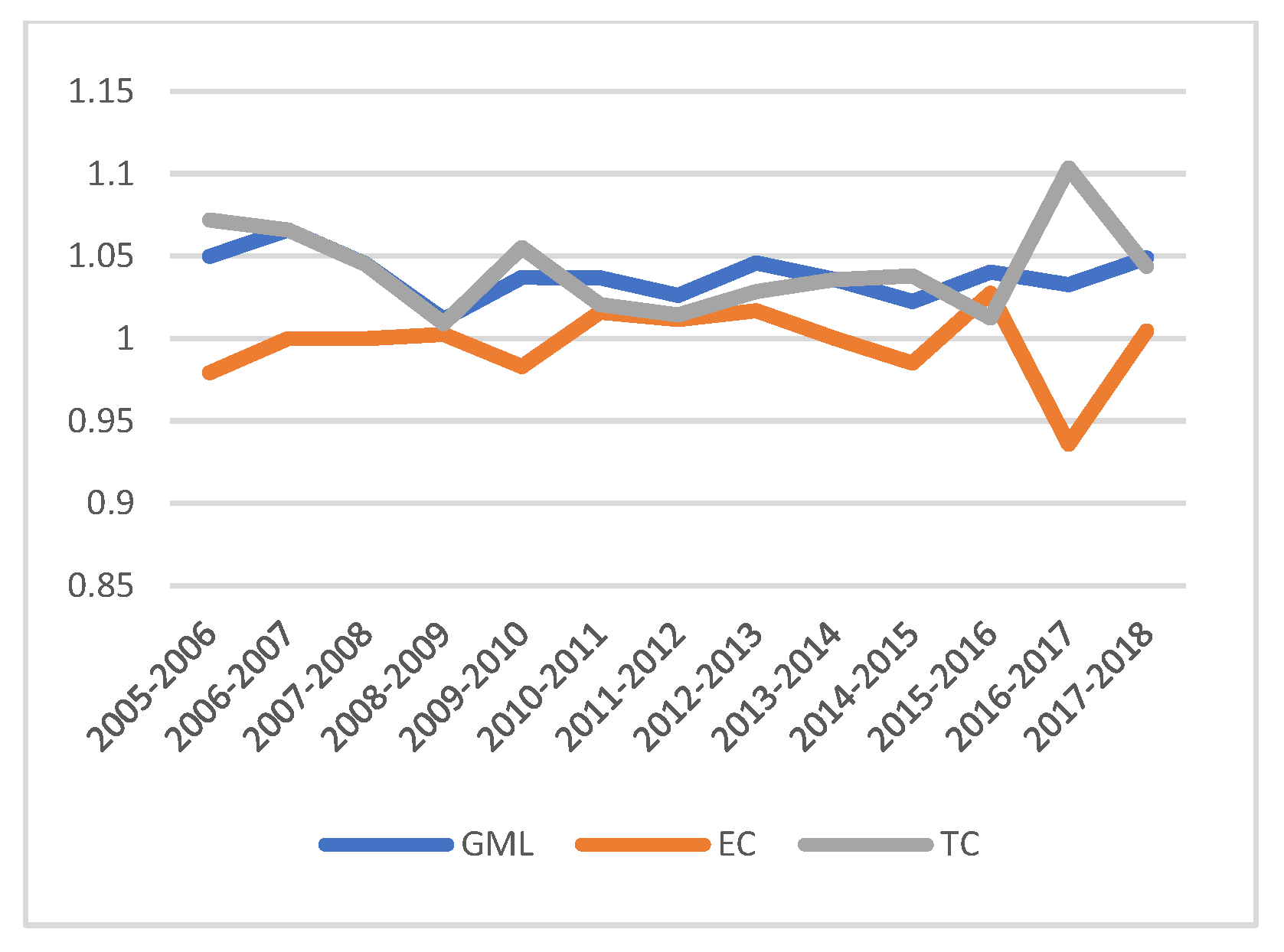
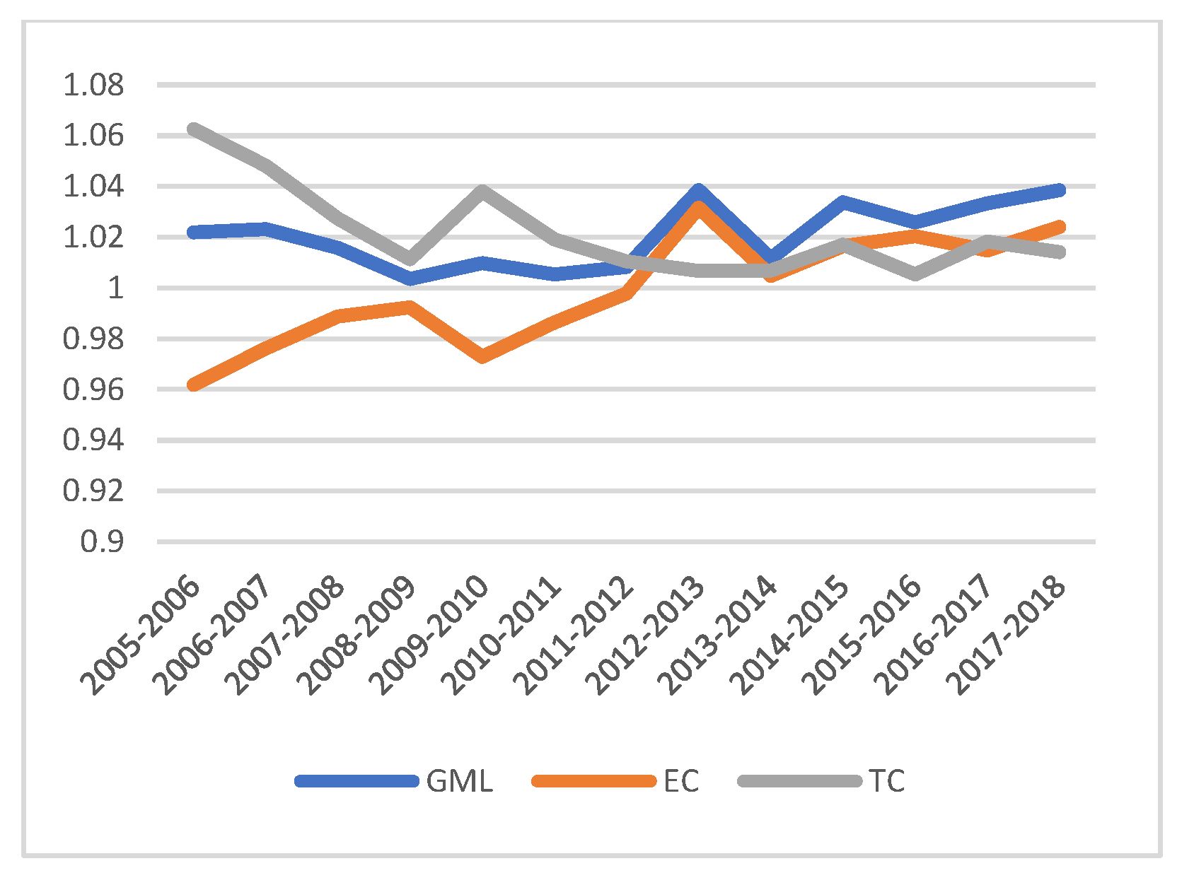
Figure 1, Figure 2, Figure 3 and Figure 4 depict the changing trend of the geometric mean of the GML index and its decomposition items in each year. Starting from the national average level, the mean value of the GML index in each year is >1, indicating an increasing trend for GTFP in each year. Overall, economic development is compatible with the implementation of environmental policies, such as energy conservation and emission reduction. The annual mean value of technological progress decomposed by the GML index is >1, while the mean value of technological efficiency in most years is <1, indicating that China’s GTFP improvement still depends on technological innovation [29] and that inefficiency hinders GTFP. From a regional perspective, GTFP growth in the eastern, central, and western areas is technology-driven, and its growth is high in the east and low in the west. The eastern region has the greatest advantage in sustainable development.

3.1.2. Explanatory Variables

In terms of the core explanatory variables, previous studies on transport infrastructure have usually considered railway and road density but ignored the transport service level of the transport infrastructure, which fails to fully represent the level of the transport infrastructure in each province. Considering that road and railway transport, respectively, account for 94.1% and 83.6% of passenger and freight transport modes in China, the transport infrastructure indicators in this paper are road density, rail density, highway service level, and railway service level. Traffic density more intuitively reflects the scale of the transportation infrastructure in each province at a quantitative level. It is represented by the stock index and is measured by the ratio of traffic mileage to the administrative area of each province. The traffic service level reflects the quality of the service provided by the transportation infrastructure. The transportation service level is calculated using the three aspects of passenger volume, freight volume, and the number of workers in the transportation business, using the entropy method. Passenger volume reflects both the provinces’ traffic infrastructure services by the number of passengers and the provinces’ goods transport infrastructure services. Freight volume belongs to the service industry; because of its relatively sharp market features and characteristics of early opening, there is a greater number of traffic services staff, which is an important indicator of the transportation service level.

3.1.3. Control Variables

To accurately analyze the impact of the transportation infrastructure on GTFP, we use four control variables: foreign direct investment (FDI); fiscal expenditure (Gov); human capital (Hum); and population density (Indens). Foreign investment may create “paradise pollution” (as developed areas have high requirements for the environment, and some enterprises create high levels of pollution, they will move to the areas that need to develop the economy, and the polluting industries will gather, resulting in the pollution of “paradise”) when expanding economic output through technology spillover [40]. This paper measures the converted FDI in the total social fixed asset investment [18]. Government fiscal expenditure is a key component of both short- and long-term macro-control, particularly in the steady growth of the economy and society. It serves as a crucial assurance to advance social progress and social fairness. The proportion of government fiscal expenditure to GDP serves as the conceptual foundation for this investigation. Human capital economic theory holds that human capital grows through the accumulation of regional knowledge and technology, subsequently stimulating economic growth. In this paper, the average number of years of education in each region is obtained by weighting the number of people aged six years old and over at different educational levels in each region. In terms of the population variable, the continuous expansion of the population promotes regional economic development, but can also increase the environmental burden. Here, we measure the ratio of population to the administrative area at the end of each year in terms of the number of people per unit area.

3.1.4. Data Sources

The data were obtained from the China Statistical Yearbook, the China Traffic Statistical Yearbook, the China Energy Statistical Yearbook, the China Environmental Statistical Yearbook, and the Provincial Statistical Yearbooks. Because of the lack of availability of data, this study did not include Tibet, Taiwan, Hong Kong, or Macao. The descriptive statistics for each indicator are shown in Table 2.

3.2. Specifications of the Spatial Econometric Model

Considering that the external effects of transportation facilities in the construction process are not only limited to the provinces but also exist among provinces, in order to analyze the spatial spillover influence of the transportation system on GTFP of neighboring provinces, this paper constructs a spatial Durbin model (9), a spatial error model (10), and a spatial lag model (11), which include the influence of GTFP and explanatory variables for neighboring provinces:
G T F P i t = α 0 + ρ W G T F P i t + α 1 K t i t + α 2 W K t i t + α 2 X i t + α 2 W X it + u i + v t + ε i t
G T F P i t = α 0 + ρ W G T F P i t + α 1 K t i t + α 2 X i t + u i + v t + ε i t
G T F P i t = α 0 + α 1 K t i t + α 2 X i t + u i + v t + ε i t , ε i t = λ W ε i t + μ i t
where i represents the province; t . represents the year; G T F P i t is the explained variable; K i t is the transportation infrastructure variable; X i t is a control variable; and ρ , λ , α 0 , u i , v t , and ε i t are the spatial autocorrelation coefficient, spatial error coefficient, constant term, spatial effect, time effect, and random disturbance term, respectively. α 1 and α 2 are parameter estimation coefficients, and W is a spatial weight matrix. In the study of the spatial effect, it is necessary to introduce a spatial weight matrix to represent the proximity of each region. This paper uses three kinds of spatial weight matrices: the adjacency matrix, W1; the anti-geographic distance matrix, W2; and the economic geographic distance matrix, W3.

4. Results Analysis

4.1. Spatial Autocorrelation Test

The variables are spatially dependent, which is the basis for discussing spatial influence. Therefore, it is necessary to test the spatial autocorrelation of the explained variables. The most common method to achieve this is to use the Moran index. This paper tests the spatial correlation between the explanatory variables and explained variables based on the adjacency matrix, W1. The results in Table 3 show that there is a significant spatial positive correlation between China’s GTFP and transportation infrastructure each year, showing the characteristics of high-value and low-value agglomeration. With the increase in years, the Moran index of GTFP shows an upward trend, the positive agglomeration characteristic of highway density is the most obvious, and the spatial correlation between railway and highway transportation capacity is weakened.
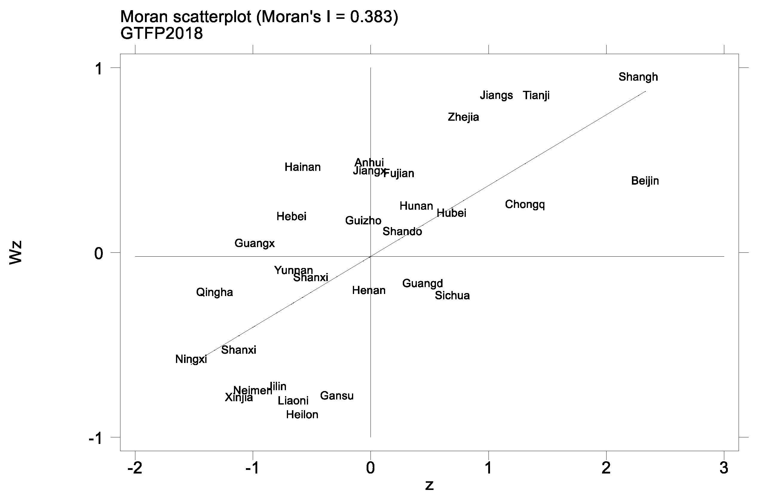
The Moran’s I plot in Figure 5 reflects the local characteristics of variables. In 2018, the spatial positive correlation of GTFP in China was found to be significant, and GTFP in most provinces was concentrated in the first and third quadrants. Among the 10 provinces in the first quadrant, eight provinces are in the eastern region, which is a high-value cluster, indicating that provinces with high GTFP levels can often promote the development of surrounding areas. Provinces in the third quadrant are mainly western regions, which are low-value clusters, indicating that areas with relatively weak GTFP levels tend to hinder the development of surrounding areas. It can be seen that GTFP in China shows the characteristics of a massive cluster in space. At the same time, the density of railways and highways in central and eastern provinces is also ranked top in China, while the density in central and western regions is lower. The spatial distribution characteristics of transportation infrastructure and GTFP are similar, and there is a close connection.

4.2. Selection of the Spatial Econometric Model

Based on the Lagrange multiplier (LM) test and its robustness in exceeding the 1% significance level, as well as to test the adaptability of the spatial Durbin model (SDM) using the Hausman test, Wald test, and likelihood-ratio (LR) test, this paper uses an SDM with a mixed fixed effect for fitting. In Table 4, the spatial autoregressive coefficient of GTFP in the results, ρ , is significantly positive, indicating that the GTFP of each province drives the GTFP of adjacent provinces. Under a series of environmental protection policies, such as energy conservation and emission reduction, the improvement in resource allocation efficiency and green technology innovation brought about by coordinated development among provinces promotes the overall GTFP. At the same time, the spatial transmission effect of explanatory variables also affects GTFP.

4.3. Direct and Indirect Effects

There is a systematic bias when measuring the spatial spillover impact of explanatory factors using the model estimate coefficient since the spatial autocorrelation coefficient of GTFP is notably not 0. As a result, this research reduces the coefficients of explanatory variables into direct impact, indirect effect, and total effect [39] based on the partial differential technique suggested by LeSage [41]. Whereas the indirect effect shows the spatial spillover effect of local explanatory variables on GTFP in nearby provinces, the direct effect, or local effect, reflects the effect of local explanatory variables on local GTFP (refer Table 5).
The results show that the spatial spillover effect of transportation infrastructure is greater than the direct effect. The direct effect, indirect effect, and total effect of road density and railway density are significantly positive (p < 0.01). At the same time, the traffic density drives the GTFP of this province and neighboring provinces, which has a positive spatial spillover effect. On the whole, the findings show that resources after the completion of China’s transportation facilities have been effectively utilized, rather than being idle resources. Sufficient transportation resources reduce transportation costs and promote the market size effect, thus improving GTFP in each region. Among them, the estimated value of each effect of highway density is less than that of railway density. Due to the early development of highways in China, regional highways are relatively complete, and their coverage area has become saturated. The continuous expansion of highway mileage construction makes the marginal efficiency increase smaller. At the same time, China’s traffic construction is focusing more on the railway. The spillover effect of railway mileage construction on GTFP in neighboring provinces is greater than the direct effect, indicating that the spillover effect brought about by the expansion of the scale of railway construction is more obvious among provinces, showing the characteristics of increasing marginal returns [42].
There are significant differences between highway and railway traffic service levels measured by passenger and freight volume and the number of employees. The direct and indirect effects of highway service level are significantly positive, which is consistent with the analysis of the current situation of relevant highway service indicators above. Highway service occupies a dominant position in the transportation service industry. For commuters and people on short business trips, cars can be used as a means of transportation to stop and start at any time, which greatly improves the service level of highways. Road transport services drive the GTFP of the region and its neighboring regions by promoting resource flow and technology spillover. However, the rail service level of direct and indirect effects is significantly negative. This may be due to the railway’s high technical requirements; compared to highways, railway construction entails a higher cost, a longer period, and more employees, while areas restricted by a poor geographical position and a lack of funds do not have a rail link, as well as having less access to highways, so the rail service level needs to be improved. At the same time, some provinces have failed to use energy efficiently and reduce pollution emissions while increasing output from the expansion of railway construction. On the one hand, due to the large volume of railway transportation, low transportation cost, and a large amount of railway cargo transportation, the pollution brought about by the transportation of goods has caused a certain burden on the ecological environment of various regions. Railways also cost more to maintain than roads, so the level of rail service does not contribute to the growth of GTFP. On the other hand, in order to join the ranks of provinces with strong transportation, provinces are continuing to strengthen railway construction and improve service levels, and resources are reallocated among regions. There are obvious competition effects among regions, which produce negative spatial spillover effects on neighboring regions and inhibit the GTFP of neighboring provinces.
The results for the control variables show that FDI inhibits the GTFP of each province and its adjacent provinces. The “paradise pollution” hypothesis holds that investors prefer to invest in provinces with low environmental regulatory requirements and relatively rich resources, resulting in increased pollution in the investment areas [40]; enterprises in these provinces may also be squeezed out of the market by aggressive competition. When the expected output does not keep pace with the increase in unexpected output and resource consumption, this inhibits GTFP. Government functions have improved the province’s GTFP, and fiscal expenditure is mostly used for external capital investment, such as infrastructure construction. As the supervisor of regional enterprise environmental regulations, the government has effectively promoted the progress of green technology in each province. At the same time, the driving role of the government has promoted the GTFP of neighboring provinces. With the improvement in the education level of each province, the environmental protection attitudes of technicians have been strengthened, which makes them pay more attention to the effective utilization of energy and pollutant discharge in developing and applying new technology, which significantly improves the GTFP of the province. However, human capital has failed to significantly affect the GTFP of neighboring provinces, indicating that there are regional limitations in the radiation range of human capital externalities in China [18]; on the whole, the positive impact of human capital is not significant. The population agglomeration effect brought about by population expansion ensures that each region has sufficient labor resources. While the specialization and division of labor are guaranteed, this also creates a market effect, which effectively promotes GTFP in each province. However, too large a population size will inevitably lead to the overuse of resources, exacerbate regional energy use and environmental pollution, and inhibit the GTFP of adjacent provinces.

4.4. Robustness Test

To test the robustness of the empirical results, this paper adopts the approach of fitting the model of the anti-geographic distance matrix, W2, and the economic geographic distance matrix, W3, as shown in Table 6.
The test results show that, under mixed fixed effects, the SDM must be selected. The results of explanatory variable decomposition show that the impact of transportation infrastructure on GTFP is the same under different weight matrices.

4.5. Regional Heterogeneity

The heterogeneity of the transport infrastructure in different regions is studied based on the adjacency matrix (Table 7). In terms of service level, the railway service level in the east and west regions is significantly negative, indicating that the railway service level inhibits the GTFP of each province and its neighboring provinces. However, the effects of the railway service level in the central region are not significant, which indicates that, although the railway promotes the technical exchange and resource factor flow in the regions along the railway, it is generally long-distance transportation, with a large cargo volume, unable to provide a sustainable service, and the lack of rationality in planning leads to environmental pollution and the ineffective use of resources, which inhibits the GTFP of the provinces in the region. There is a positive spillover effect of highway transportation capacity only in the central and western regions, indicating that the cross-regional resource flow brought about by the highway is more prevalent. In terms of traffic density, the highway density in the eastern region inhibits the GTFP of the province and its neighboring provinces, while the effects of railway density in the central and western regions are significantly negative. Although the highway density in the eastern provinces shows absolute advantages, the intensive highway construction reduces the marginal rate of return [30]. The rich resources and developed economy in the region also produce strong competition, and too aggressive competition will have negative effects on GTFP. Because of the low density and uneven distribution of railways in central and western China, there are still many areas with negative externalities in railway transport.

4.6. Discussion

Two research hypotheses were proposed in Section 2: H1: Traffic network density is conducive to the improvement of GTFP; and H2: The traffic service level is conducive to the improvement of GTFP, but it may also be inhibited by negative externalities. This paper has studied the impact of transportation infrastructure on GTFP through the spatial econometric model, and the empirical analysis results were found to be consistent with the research hypotheses. Consistent with previous studies, road density, rail density, and road service level drive GTFP. However, previous research has mainly focused on the highway, therefore largely ignoring the railway service level, in studying GTFP, which represents an innovation of the present paper.

5. Conclusions and Implications

Based on the SBM and GML indices, we calculated the GTFP of Chinese provinces, revealing an increasing trend year by year. This paper analyzed the spatial spillover effect of China’s transport infrastructure on GTFP from two perspectives: the scale of transport facilities’ construction; and the level of transport services. The spatial spillover influence of the interprovincial transportation structure was found to be significant. Road density, railway density, and road service level were found to have positive effects on the GTFP of the whole province and its neighboring provinces, and the total effects were 1.72, 39.56, and 1.968, respectively. The estimated effects of road density were smaller than those of railway density, and the spatial spillover effect of railway density was 33.16 and greater than the direct effect of 6.40. Each unit improvement in railway service level thus reduces the GTFP of neighboring provinces by 0.63 units. The results of the regional division showed that the transport infrastructure has obvious regional heterogeneity. Railway density in the central and western regions and road density in the eastern regions inhibit GTFP in the respective regions and surrounding provinces. The direct spillover effect and spatial spillover effect of highway service level in eastern China were found to be significantly positive, while the spillover effect was found to exist only in central and western China. The railway service level in the east, middle, and west has an inhibitory effect on the GTFP of the whole province and its neighboring provinces. Among the control variables, foreign direct investment inhibited GTFP, while government function, human capital, and population size significantly inhibited GTFP. Thus, only government functions have positive spillover effects.
Based on our results, we conclude that all regions need to improve the scale and quality of their transportation infrastructure. At present, the network density of various grades of highways has increased overall, but the railway mileage, especially for high-speed rail construction, needs to be extended further to obtain a higher marginal rate of return. At the same time, we should pay more attention to the quality of transportation construction by continuously improving the service level. In addition, timely maintenance needs to be carried out with the continuing development of railway facilities prone to environmental pollution. There should be increases in China’s traffic-carrying capacity, coordinated expansion of railway transportation systems in the region, and improvements in railway transportation capacity. All of these plans should focus on eliminating bottlenecks that hinder GTFP in the various provinces. Second, reasonable plans should be drafted for traffic construction in the various regions to narrow the traffic development gap. The eastern region should not blindly pursue “extensive” traffic construction but should pay more attention to the problem of diminishing marginal income caused by dense highway construction. When the traffic flow is small, the resources in the region cannot be fully utilized and, when the traffic flow is large, the pollution in the region will increase. The central and western areas should increase the construction of railway facilities, constantly optimize the spatial layout of railways, promote the effective allocation of resources through the “space-time compression” characteristics of railways, and focus more on coordinating railway construction with environmental stewardship. At the same time, all regions should pay attention to the importance of traffic construction in the quality of economic growth and continuously improve the scale and quality of traffic construction. Finally, to create a good environment for sustainable development, all regions should work together to adopt strong measures for promoting GTFP. While continuously improving the transportation infrastructure, the government should also increase investment in environmental pollution control. Policy makers need to formulate reasonable environmental regulation policies, including minimizing the “paradise pollution” brought about by foreign investment. The radiation scope of knowledge and technology spillover must be enhanced together with the effective utilization of human resources and the rational flow and agglomeration of the population in the region. Only in this way can China ultimately achieve the coordinated development of resources, the environment, and the economy.

Author Contributions

Conceptualization, J.W.; data curation, X.Y.; formal analysis, S.K.; funding acquisition, J.W.; investigation, S.K.; methodology, X.Y.; project administration, J.W.; resources, J.W.; software, X.Y. and S.K.; visualization, S.K.; writing—original draft, J.W. and X.Y. All authors have read and agreed to the published version of the manuscript.

Funding

This research was supported by the National Social Science Foundation of China (21BTJ050), the National Statistical Research Program of China (Project No. 2021LY066), the High-Level Talents Project of Jiangsu University (Project No. 12JDG009), and the Postgraduate Research & Practice Innovation Program of Jiangsu Province (Project No. KYCX20_3056).

Institutional Review Board Statement

Not applicable.

Informed Consent Statement

Not applicable.

Data Availability Statement

Data will be available upon request from the authors.

Conflicts of Interest

The authors declare no conflict of interest.

References

  1. Smith, A. The Essential Adam Smith; WW Norton & Company: New York, NY, USA, 1987. [Google Scholar]
  2. Guo, G.; Liu, R.; Huang, Z. Economic Growth Model of Transportation Infrastructure Affecting Consumption. Econ. Res. 2019, 54, 166–180. (In Chinese) [Google Scholar]
  3. Xun, Z.; Xu, W.; Guanghua, W.; Fangcheng, S. A Comprehensive Framework for Transportation Infrastructure to Promote Economic Growth. J. Econ. Res. 2018, 15, 5–23. [Google Scholar]
  4. Wang, L.; Zhai, B. Impact of transportation infrastructure on economic growth in the Yangtze River economic belt. Resour. Environ. Yangtze River Basin 2018, 27, 6–12. [Google Scholar]
  5. Celbis, M.G.; de Crombrugghe, D. Internet infrastructure and regional convergence: Evidence from Turkey. Pap. Reg. Sci. 2018, 97, 387–409. [Google Scholar] [CrossRef]
  6. Arbués, P.; Baños, J.F.; Mayor, M. The spatial productivity of transportation infrastructure. Transp. Res. Part A Policy Pract. 2015, 75, 166–177. [Google Scholar] [CrossRef]
  7. Park, J.S.; Seo, Y.-J.; Ha, M.-H. The role of maritime, land, and air transportation in economic growth: Panel evidence from OECD and non-OECD countries. Res. Transp. Econ. 2019, 78, 100765. [Google Scholar] [CrossRef]
  8. Marinos, T.; Belegri-Roboli, A.; Michaelides, P.G.; Konstantakis, K. The spatial spillover effect of transport infrastructures in the Greek economy (2000–2013): A panel data analysis. Res. Transp. Econ. 2022, 94, 101179. [Google Scholar] [CrossRef]
  9. Nguyen, H.M. Spatial Spillover Effects of Transport Infrastructure on Economic Growth of Vietnam Regions: A Spatial Regression Approach. Real Estate Manag. Valuat. 2022, 30, 12–20. [Google Scholar] [CrossRef]
  10. Shabani, Z.D.; Safaie, S. Do transport infrastructure spillovers matter for economic growth? Evidence on road and railway transport infrastructure in Iranian provinces. Reg. Sci. Policy Pract. 2018, 10, 12114. [Google Scholar]
  11. Wang, C.; Lim, M.K.; Zhang, X.; Zhao, L.; Lee, P.T.-W. Railway and road infrastructure in the Belt and Road Initiative countries: Estimating the impact of transport infrastructure on economic growth. Transp. Res. Part A Policy Pract. 2020, 134, 288–307. [Google Scholar] [CrossRef]
  12. Farhadi, M. Transport infrastructure and long-run economic growth in OECD countries. Transp. Res. Part A Policy Pract. 2015, 74, 73–90. [Google Scholar] [CrossRef]
  13. Ezcurra, R.; Gil, C.; Pascual, P.; Rapún, M. Public capital, regional productivity and spatial spillovers. Ann. Reg. Sci. 2005, 39, 471–494. [Google Scholar] [CrossRef] [Green Version]
  14. Kailthya, S.; Kambhampati, U. Road to productivity: Effects of roads on total factor productivity in Indian manufacturing. J. Comp. Econ. 2022, 50, 174–195. [Google Scholar] [CrossRef]
  15. Cheng, Z.; Chai, Y. Transportation infrastructure, foreign trade and total factor productivity. East China Econ. Manag. 2021, 35, 91–99. [Google Scholar]
  16. Zhang, X.; Chen, L.; Wu, W. Transportation infrastructure, hierarchical agglomeration of human capital and regional total factor productivity—An Empirical Analysis based on the panel data of 285 prefecture level cities in China. Ind. Technol. Econ. 2016, 35, 92–102. [Google Scholar]
  17. Chen, W.; Pan, Y.; Ma, L. Transportation infrastructure, spatial spillover and total factor productivity—Spatial econometric analysis based on panel data of the Silk Road Economic Belt. Ind. Technol. Econ. 2017, 36, 22–30. [Google Scholar] [CrossRef]
  18. Haoran, Z.; Baozhong, Y. Infrastructure, spatial spillover and regional total factor productivity—Based on Chinese 266 urban spatial panel Durbin model study. Economist 2012, 2, 61–67. [Google Scholar]
  19. Wang, X.; Zhang, K. One belt, one road, provinces, infrastructure investment and total factor productivity. Jiangxi Soc. Sci. 2018, 38, 30–39. [Google Scholar]
  20. Wang, R.; Ou, G.; Wang, Q. Can trade liberalization improve total factor productivity—Analysis based on the regulation effect of transportation infrastructure. J. Beijing Jiaotong Univ. Soc. Sci. Ed. 2019, 18, 38–47. [Google Scholar]
  21. Qalati, S.A.; Kumari, S.; Tajeddini, K.; Bajaj, N.K.; Ali, R. Innocent devils: The varying impacts of trade, renewable energy and financial development on environmental damage: Nonlinearly exploring the disparity between developed and developing nations. J. Clean. Prod. 2023, 386, 135729. [Google Scholar] [CrossRef]
  22. Kumari, S.; Rajput, S.K.O.; Soomro, N.A.; Ali, R.; Ghumro, N.H. Role of renewable energy consumption, financial development and FDI in promoting trade and sustainability: Evidence from SAARC region. Acad. Account. Financ. Stud. J. 2022, 26, 1–15. [Google Scholar]
  23. China Mobile Limited. Sustainability Report. Digitalized and Intelligent New Power for All. 2020. Available online: https://www.chinamobileltd.com/en/ir/reports/ar2020/sd2020.pdf (accessed on 1 March 2023).
  24. Qalati, S.A.; Kumari, S.; Soomro, I.A.; Ali, R.; Hong, Y. Green supply chain management and corporate performance among manufacturing firms in Pakistan. Front. Environ. Sci. 2022, 540, 873837. [Google Scholar] [CrossRef]
  25. Vlahinić Lenz, N.; Pavlić Skender, H.; Mirković, P.A. The macroeconomic effects of transport infrastructure on economic growth: The case of Central and Eastern E.U. member states. Econ. Res. Ekon. Istraz. 2019, 31, 1953–1964. [Google Scholar] [CrossRef]
  26. Wetwitoo, J.; Kato, H. Inter-regional transportation and economic productivity: A case study of regional agglomeration economies in Japan. Ann. Reg. Sci. 2017, 59, 321–344. [Google Scholar] [CrossRef]
  27. Solow, R.M. Technical Change and the Aggregate Production Function. Rev. Econ. Stat. 1957, 39, 554–562. [Google Scholar] [CrossRef] [Green Version]
  28. Zha, Q.; Huang, C.; Kumari, S. The impact of digital economy development on carbon emissions—Based on the Yangtze River Delta urban agglomeration. Front. Environ. Sci. 2022, 10, 2033. [Google Scholar] [CrossRef]
  29. Wang, B.; Liu, G. Energy Saving and Emission Reduction and China’s Green Economy Growth: A Perspective of Total Factor Productivity. China Ind. Econ. 2015, 5, 57–69. [Google Scholar]
  30. Krugman, P. Increasing Returns and Economic Geography. J. Political Econ. 1991, 99, 483–499. [Google Scholar] [CrossRef]
  31. Xu, H.; Xu, S.; Zhang, B. The impact of transportation infrastructure on green Total Factor Productivity: From the perspective of threshold Effect. Ecol. Econ. 2020, 36, 69–73+85. [Google Scholar]
  32. Liu, B.; Wu, P.; Jason, L. The traffic infrastructure and the total factor productivity growth in China—Panel econometric analysis based on the provincial data space. China’s Ind. Econ. 2010, 3, 54–64. [Google Scholar]
  33. Zhang, J.; Zheng, J. Whether China’s economic growth falls into the trap of “Baumol’s Disease”—Reflection on the negative Effect of Highway infrastructure Investment on Regional Total Factor Productivity. J. Nanjing Univ. Philos. Hum. Sci. Soc. Sci. 2022, 59, 26–52+158. [Google Scholar]
  34. Kumari, S.; Oad Rajput, S.K.; Hussain, R.Y.; Marwat, J.; Hussain, H. Optimistic and pessimistic economic sentiments and US Dollar exchange rate. Int. J. Financ. Eng. 2022, 9, 2150043. [Google Scholar] [CrossRef]
  35. Fare, R.; Primont, D. Multi-Output Production and Duality: Theory and Applications: Theory and Applications; Springer Science & Business Media: New York, NY, USA, 1994. [Google Scholar]
  36. Tone, K. A slacks-based measure of efficiency in data envelopment analysis. Eur. J. Oper. Res. 2001, 130, 498–509. [Google Scholar] [CrossRef] [Green Version]
  37. Zhang, J.; Wu, G.; Zhang, J. Estimation of China’s inter-provincial physical capital stock: 1952–2000. Econ. Res. J. 2004, 10, 35–44. [Google Scholar]
  38. Wei, C.; An-Wei, W.; Kumari, S. Do more get more: Monopoly appropriation of labor income in manufacturing companies. Front. Environ. Sci. 2022, 10, 2275. [Google Scholar] [CrossRef]
  39. Qiu, B.; Yang, S.; Xin, P. FDI Technology Spillover channels and productivity growth in China’s manufacturing industry: An analysis based on panel Data. World Econ. 2008, 8, 20–31. [Google Scholar]
  40. Gong, C.; Zhang, X. The spatial effect of China’s Interregional environmental regulation on green economic efficiency and its decomposition. Discuss. Mod. Econ. 2020, 4, 41–47. [Google Scholar]
  41. LeSage, J.P. An Introduction to Spatial Econometrics. Rev. Écon. Ind. 2008, 123, 3887. [Google Scholar] [CrossRef] [Green Version]
  42. Wen, H.; Han, X. The impact of high-speed railways on urban accessibility and regional economic spatial pattern in China. Hum. Geogr. 2017, 32, 99–108. [Google Scholar]
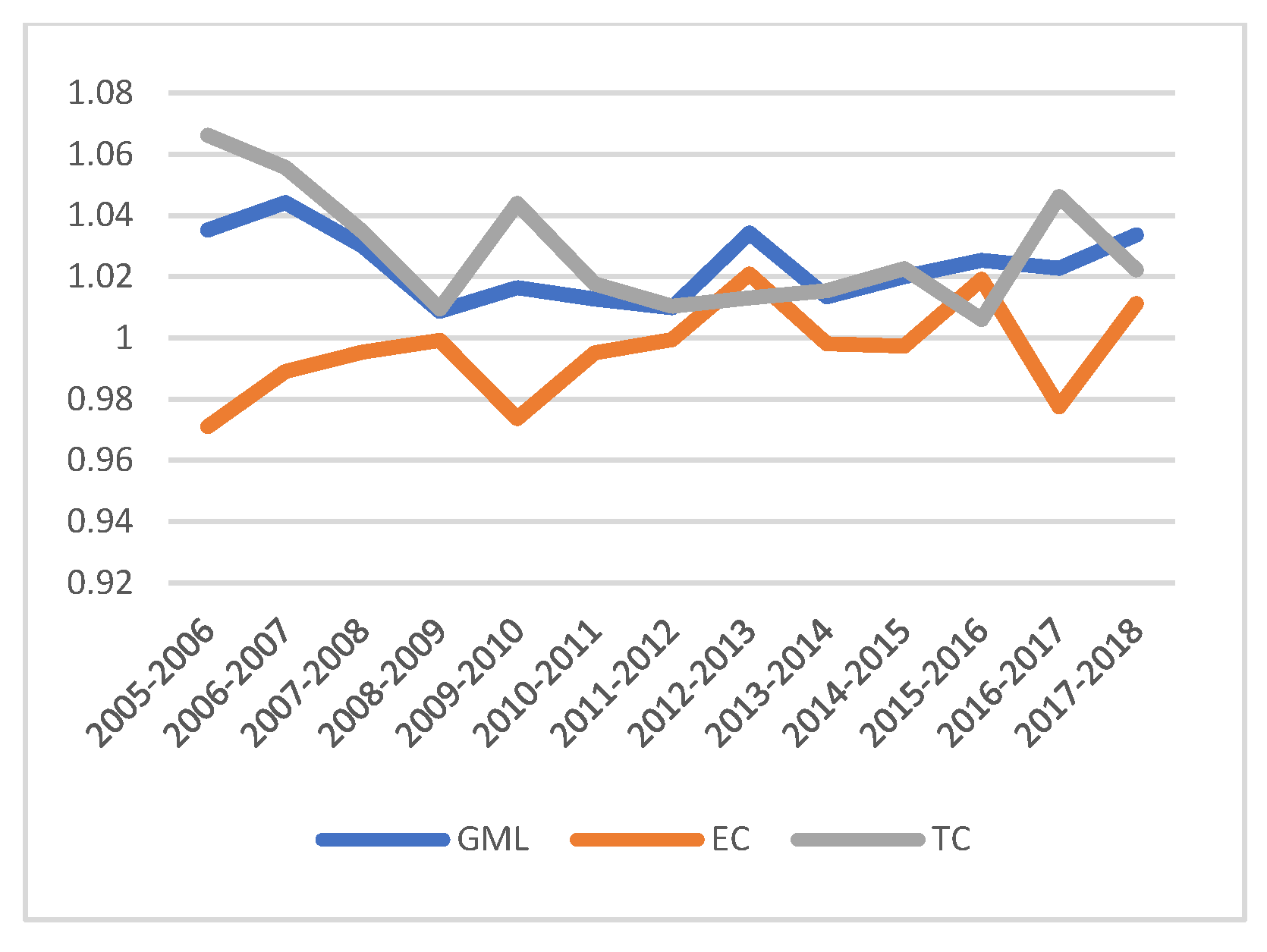
Figure 1. Trends of GML and its decomposition index in China from 2006 to 2019.
Energies 16 02733 g001
Figure 2. Trends of GML and its decomposition index in eastern China from 2006 to 2019.
Energies 16 02733 g002
Figure 3. Trends of GML and its decomposition index in central China from 2006 to 2019.
Energies 16 02733 g003
Figure 4. Trends of GML and its decomposition index in western China from 2006 to 2019.
Energies 16 02733 g004
Figure 5. Moran’s I plot of GTFP in 2018.
Energies 16 02733 g005
Table 1. Descriptive statistics for each indicator.
VariableMeanStd. Dev.Min.Max.
Actual GDP (100 million yuan)12,085.0911,050.27461.7567,945.49
Capital stock (100 million yuan)36,916.7330,406.562336.75163,132.30
Years of education of the labor force (years)9.461.266.4613.50
Energy consumption (ten thousand tons)13,056.908274.84822.0040,581.00
SO2 emissions (ten thousand tons)63.1144.890.27200.20
Production of industrial solid waste (ten thousand tons)9346.278659.84127.0048,541.30
Discharge of wastewater (ten thousand tons)214,206.40170,277.4019,360.00938,261.00
Wastewater discharge (ten thousand tons)37,667.0730,339.991249.17179,336.90
Table 2. Descriptive statistics for each indicator.
VariableMeanStd. Dev.Min.Max.
GTFP1.2103010.27262940.77154262.36518
Road0.8697340.47825150.06619282.10093
Rail0.02442740.02007580.00175690.0967861
Rail service level0.18144310.12798730.00217530.5929346
Road service level0.18432970.15106680.01603390.8689324
FDI0.04084640.04243070.00007080.2296779
Indens5.440841.2730122.0282218.249705
Gov0.23766670.10993960.09478220.7582924
Hum8.8453380.98697836.59396112.55503
Table 3. The Moran index of green total factor productivity (GTFP) and transportation infrastructure.
YearGTFPRoadRailRail Service LevelRoad Service Level
20060.181 **0.585 ***0.423 ***0.213 **0.340 ***
20070.128 *0.580 ***0.423 ***0.178 **0.355 ***
20080.0980.588 ***0.418 ***0.236 **0.297 ***
20090.248 ***0.593 ***0.442 ***0.251 ***0.250 ***
20100.274 ***0.592 ***0.377 ***0.215 **0.240 ***
20110.323 ***0.596 ***0.386 ***0.183 **0.191 **
20120.341 ***0.602 ***0.371 ***0.207 **0.195 ***
20130.355 ***0.609 ***0.380 ***0.173 **0.162 **
20140.378 ***0.586 ***0.368 ***0.230 **0.154 **
20150.354 ***0.578 ***0.372 ***0.182 **0.188 **
20160.371 ***0.579 ***0.354 ***0.199 **0.207 ***
20170.374 ***0.583 ***0.355 ***0.177 **0.211 ***
20180.383 ***0.583 ***0.346 ***0.163 **0.231 **
Note: ***, **, and * indicate statistical significance at the 1%, 5%, and 10% levels, respectively.
Table 4. Estimation results of the SDM, SEM, and SAR models of transport infrastructure affecting green total factor productivity (GTFP).
SDMSEMSAR
VariableEstimated Valuet-ValueEstimated Valuet-ValueEstimated Valuet-Value
Road0.468 ***4.930.489 ***4.740.495 ***5.37
Rail4.083 *2.302.9331.564.921 **2.79
Rail service level−0.524 **−2.87−0.596 **−3.08−0.775 ***−4.06
Road service level0.711 ***7.570.679 ***7.070.716 ***7.50
FDI−0.683 *−2.440.003050.01−0.165−0.59
Indens0.896 ***4.210.779 ***3.670.474 **2.81
Gov0.241.29−0.349−1.83−0.214−1.15
Hum0.0863 **2.920.0884 **2.810.0840 **2.69
W × Road0.550 **2.90
W × Rail19.62 ***5.16
W × Rail service level−0.815 *−2.21
W × Road service level0.460 *2.22
W × FDI−1.748 ***−4.34
W × Indens−1.703 ***−4.59
W × Gov0.879 **2.67
W × Hum−0.0173−0.25
ρ 0.394 ***6.14 0.563 ***10.71
λ 0.560 ***8.83
Sigma20.00692 ***13.710.00873 ***13.270.00803 ***13.44
R-squared0.55930.59890.5851
log-likelihood408.3818353.7576370.1923
N390390390
Hausman14.33 ***
Wald-lag78.68 ***
Wald-err119.56 ***
LR-lag76.38 ***
LR-err109.25 ***
Note: ***, **, and * indicate statistical significance at the level of 1%, 5%, and 10%, respectively.
Table 5. Direct, indirect, and total effects of transportation infrastructure and control variables on green total factor productivity (GTFP).
VariableDirect EffectIndirect EffectTotal Effect
Estimated Valuet-ValueEstimated Valuet-ValueEstimated Valuet-Value
Road0.555 ***5.571.164 ***4.091.720 ***5.37
Rail6.402 ***3.4333.155 ***5.2339.556 ***5.38
Rail service level−0.625 ***−3.19−1.604 ***−2.7−2.229 ***−3.1
Road service level0.796 ***8.011.172 ***3.331.968 ***4.83
FDI−0.911 ***−3.12−3.162 ***−4.76−4.073 ***−4.74
Indens0.758 ***3.8−2.091 ***−3.99−1.334 ***−2.66
Gov0.350 *1.681.523 ***2.931.872 ***2.95
Hum0.087 ***2.780.0270.240.1140.88
Note: ***, and * indicate statistical significance at the level of 1%, and 10%, respectively.
Table 6. Results of the robustness test.
MatrixVariableDirect EffectIndirect EffectTotal Effect
Estimated Valuet-ValueEstimated Valuet-ValueEstimated ValueI-Value
Anti−geographical distance matrix, W2Road0.784 ***7.421.785 ***4.312.569 ***5.49
Rail8.348 ***4.4641.85 ***6.0650.20 ***6.54
Rail service level−0.484 **−2.41−1.392 *−2.34− 1.876 ***−2.64
Road service level0.871 ***8.431.159 ***3.512.030 ***5.35
FDI−0.591 *−1.92−0.73−0.70−1.32−1.07
Indens0.812 ***3.77−2.793 ***−4.98−1.981 ***−3.82
Gov0.483 **2.141.154 *1.941.637 **2.35
Hum0.0662 **2.070.060.470.1230.92
Economic geographical distance matrix, W3Road0.816 ***7.381.787 ***4.092.603 ***5.29
Rail9.121 ***4.6737.12 ***5.9846.24 ***6.60
Rail service level−0.558 ***−2.64−1.355 **−2.31−1.914 ***−2.67
Road service level0.865 ***8.181.027 ***−3.431.892 ***5.42
FDI−0.766 **−2.39−1.575 *−1.72−2.342 **−2.09
Indens0.887 ***4.13−2.765 ***−5.09−1.878 ***−3.69
Gov0.446 *1.881.467 **2.061.912 **2.34
Hum0.067 *1.970.07210.540.1390.95
Note: ***, **, and * indicate statistical significance at the 1%, 5%, and 10% level, respectively.
Table 7. Effect decomposition of regional transportation infrastructure based on the adjacency weight matrix.
RegionVariableDirect EffectIndirect EffectTotal Effect
Estimated Valuet-ValueEstimated Valuet-ValueEstimated Valuet-Value
Eastern regionRoad−0.588 ***−2.65−0.765 *−1.55−1.354 **−2.18
Rail8.437 ***2.697.8641.216.301 *1.87
Rail service level−1.334 ***−4.45−2.405 ***−3.99−3.740 ***−4.47
Road service level0.811 ***6.490.676 ***2.741.487 ***4.61
Central regionRoad0.342 ***3.990.623 *40.965 *5.8
Rail−7.727 ***−4.810.1570.05−7.57 **−2.07
Rail service level−0.194−0.820.2690.780.0750.22
Road service level0.0270.190.895 ***3.580.922 ***3.63
Western regionRoad0.941 ***7.172.868 ***8.493.810 ***10.7
Rail−10.893 ***−2.61−28.483 ***−3.41−39.376 ***−4.55
Rail service level−0.850 ***−3.580.230.66−0.621 **−1.74
Road service level0.1950.951.225 ***2.91.420 ***2.89
Note: ***, **, and * indicate statistical significance at the level of 1%, 5%, and 10%, respectively.
Disclaimer/Publisher’s Note: The statements, opinions and data contained in all publications are solely those of the individual author(s) and contributor(s) and not of MDPI and/or the editor(s). MDPI and/or the editor(s) disclaim responsibility for any injury to people or property resulting from any ideas, methods, instructions or products referred to in the content.