One-Day-Ahead Hourly Wind Power Forecasting Using Optimized Ensemble Prediction Methods

Abstract

This paper proposes an optimal ensemble method for one-day-ahead hourly wind power forecasting. The ensemble forecasting method is the most common method of meteorological forecasting. Several different forecasting models are combined to increase forecasting accuracy. The proposed optimal ensemble method has three stages. The first stage uses the k-means method to classify wind power generation data into five distinct categories. In the second stage, five single prediction models, including a K-nearest neighbors (KNN) model, a recurrent neural network (RNN) model, a long short-term memory (LSTM) model, a support vector regression (SVR) model, and a random forest regression (RFR) model, are used to determine five categories of wind power data to generate a preliminary forecast. The final stage uses an optimal ensemble forecasting method for one-day-ahead hourly forecasting. This stage uses swarm-based intelligence (SBI) algorithms, including the particle swarm optimization (PSO), the salp swarm algorithm (SSA) and the whale optimization algorithm (WOA) to optimize the weight distribution for each single model. The final predicted value is the weighted sum of the integral for each individual model. The proposed method is applied to a 3.6 MW wind power generation system that is located in Changhua, Taiwan. The results show that the proposed optimal ensemble model gives more accurate forecasts than the single prediction models. When comparing to the other ensemble methods such as the least absolute shrinkage and selection operator (LASSO) and ridge regression methods, the proposed SBI algorithm also allows more accurate prediction.

1. Introduction

Renewable energy will account for 20% of the total energy that is generated by 2025 in Taiwan. The target for wind turbine power capacity is 4.2 GW. The intermittent nature of the delivery of renewable energy will have a significant impact on the power system. A novel coordinated control approach is then used to offer high-quality voltages and allow optimal power transfer for a grid [1]. For an offshore wind farm that connects to the grids, the weak feeder and high harmonic characteristics have an impact on the safe operation of the system. The key technologies of transient protection for offshore wind farm transmission lines are reviewed in [2]. A study on the monitoring, operation, and maintenance of offshore wind farms is proposed to reduce the operation and maintenance costs and improve the stability of the power generation system [3].

Accurate wind power forecasting allows reliable power management and ensures an appropriate backup capacity, which reduces the cost of penetration and operation of wind power facilities. However, the variability and irregularity of wind means that forecasts are uncertain, and this affects power system management decisions. The accuracy of wind power forecasting must be increased to ensure a reliable supply of power to the grid.

The time horizon of one-day-ahead hourly forecasting of wind power is used for power management, demand response in day-ahead, load dispatch planning, and ancillary services, such as the frequency regulation reserve, the fast response reserve and the real-time spinning reserve [4]. Accurate one-day-ahead hourly wind power forecasting allows a rational power supply reserve, which reduces operating costs. Many studies propose methods for wind power forecasting. Indirect forecasting and direct forecasting are the two major categories. Indirect forecasting predicts the future wind speed based on historical wind speed and meteorological data, which includes the hidden Markov model [5], variational recurrent autoencoder [6], machine learning regression [7], dynamic integration method [8], spectrum analysis [9], hybrid machine learning model [10], stochastic method [11] and variable support segment method [12]. A power curve or a machine learning method that represents the nonlinear relationship between wind speed and corresponding wind power is then used to establish a prediction model. In this study, an indirect method is used for wind power forecasting [13].

Direct forecasting uses a physical method, a statistical method, a learning machine method, a hybrid method or an ensemble method to establish a forecasting model based on historical wind power and meteorological data. The methods for direct forecasting include a gradient-boosting machine (GBM) algorithm [14], a Bayesian optimization-based machine learning algorithm [15], an AI-based hybrid method [16], a nonparametric probabilistic method [17], an online ensemble method [18], a variable mode decomposition method [19], a multi-step method [20], a hybrid algorithm [21], an LSTM model [22], and an SVR with rolling origin recalibration [23].

Each method may feature a large forecasting error due to the variability and irregularity of the wind. To increase forecasting accuracy, an ensemble technique that combines several machine learning methods is used. Ensemble forecasting methods (EFM) were used for early meteorological forecasting and are currently used to increase the accuracy of renewable energy forecasting. An EFM combines several different forecasting models to reduce overestimation and preserve the diversity of models. The EFM uses either competition or cooperation methods [24]. The competition method uses different data sets or an individual model with the same data set but different parameters to train a model. The prediction output from each model is averaged to give a final prediction. As shown in [25], the weather variables, such as temperature, humidity, precipitation, and wind speed are regarded as individual models that affect the solar power output. A least absolute shrinkage and selection operator (LASSO) method is used to aggregate the output of each weather model. The results show that the LASSO algorithm achieves considerably higher accuracy than existing methods. A study [26] used a regression-based ensemble method for short-term solar forecasting. A random forest regression (RFR) with different parameters is used for a single forecasting method. Five RFR models are established and integrated using a ridge regression, for which the hyperparameters are tuned using a Bayesian optimization algorithm.

The cooperative method divides the prediction model into several sub-models. Depending on the characteristics of each sub-model, a prediction model is established, and the final predicted values are calculated by aggregating the outputs of each sub-model. A previous study [27] used a ridge regression method to aggregate the output of four machine learning algorithms for solar and wind power forecasts. Another study [28] used a constrained least squares (CLS) regression method to combine the wind power predictions for three single forecasting models. One study [29] used a chaos local search JAVA algorithm to aggregate the output of four machine learning networks for wind speed forecasting. Another study [30] used a weighted average method to combine the output of four single models for wind speed forecasting. A stacking ensemble method uses an ensemble neural network (ENN) [31] or a recurrent neural network (RNN) [32] to aggregate the output of several single models for solar power forecasting. The ensemble method that is mentioned avoids overfitting and gives better forecasting accuracy than a single model.

This study uses a cooperative method to evaluate five different models for one-day-ahead hourly wind power forecasting. The proposed method first uses the k-means method to divide wind power data into different clusters. Five single prediction models, including a K-nearest neighbors (KNN), an RNN, a LSTM, an SVR. and an RFR, are established to generate a preliminary forecast. An optimization technique that uses swarm-based intelligence (SBI) algorithms, such as the particle swarm optimization (PSO), the salp swarm algorithm (SSA) and the whale optimization algorithm (WOA), is used to assign a weight to each single model for every hour. The final predicted value is generated by adding the weighted sum for each individual model. To address inaccuracy in wind speed prediction from a forecasting platform, an RFR model is used to correct the forecasted values. The main contributions of this paper are as follows:

• A k-means method is used to divide historical wind power data into five different categories. Each category of data is used to establish individual forecasting models. A total of 25 sub-models (five categories of data with five single models) are established to increase forecasting accuracy by 12% to 31%.
• A cooperative method that combines the output of five single machine learning algorithms prevents overestimation and give a more accurate forecast than single prediction models.
• In contrast to existing cooperative methods, an SBI algorithm is used to optimize the weight distribution of each single model for every hour. Assigning weights for each hour is more complicated and time-consuming, but it can increase the prediction accuracy.
• One-day-ahead hourly wind speed prediction from a forecasting platform features a large error so an RFR model is used to correct the forecasted values. The proposed correction model decreases wind power forecasting error by 2–3% MRE value.

The remainder of this paper is organized as follows. Section 2 describes the existing ensemble methods. Section 3 details the proposed optimal ensemble method. Five single models are also described in this section. Section 4 describes the test results for a 3.6 MW wind power generation system. Conclusions are given in Section 5.

2. Ensemble Forecasting Methods

An EFM combines several forecasting models to increase forecasting accuracy and is widely used for meteorological forecasting. Described below are the general ensemble forecasting methods.

2.1. Weighted Average Method

The weighted average method generates prediction results by averaging the predicted outputs for each model, as [23,30]:

$$\widehat{Y}=\frac{1}{T}{\displaystyle \sum }_{i=1}^T{\widehat{y}}_i$$

(1)

where T is the number of prediction models and ${\widehat{y}}_i$ is the output from the ith prediction model.

2.2. Weighted Sum Method

The weighted sum method generates prediction results by aggregating the outputs from each sub-model with dissimilar weights [24], as:

$$\widehat{Y}=\frac{1}{T}{\displaystyle \sum }_{i=1}^T{w}_i{\widehat{y}}_i,\hspace{1em}\hspace{1em}{w}_i\ge 0,\hspace{1em}\hspace{1em}and {\displaystyle \sum }_{i=1}^T{w}_i=1$$

(2)

2.3. LASSO Regression Method

The LASSO regression is a regularization method that prevents overfitting [25,26]. A LASSO regression performs feature selection to determine predictors that contribute significantly to the model; models that contribute to a lesser extent are assigned lower weights. The LASSO regression method is expressed as:

$$\widehat{Y}={\displaystyle \sum }_{i=1}^T{w}_i\times {\widehat{y}}_i$$

(3)

The weights in (3) are calculated as:

$$\underset{w\in R^T}{\min }{\left|\right|\widehat{Y}w-Y\left|\right|}_2^2+\alpha {\left|\right|w\left|\right|}_2^2$$

(4)

The term $\left|\right|w|{|}_2^2$ represents the square root of a norm and α ≥ 0 is a penalty parameter that controls the amount of shrinkage. The greater the value of α, the greater is the amount of shrinkage, so the coefficient is more robust to collinearity.

2.4. Ridge Regression Method

Like the LASSO regression method, a ridge regression uses the square of the weight, instead of the square root of a norm [26,27], as:

$$\underset{w\in R^T}{\min }{\left|\right|\widehat{Y}w-Y\left|\right|}_2^2+\alpha w^2$$

(5)

2.5. Constrained Least Squares Regression Method

A constrained least squares regression minimizes the sum of the squared error by training the estimated outputs from several single models as [28]:

$$\widehat{Y}={\displaystyle \sum }_{i=1}^T{w}_i\times {\widehat{y}}_i+\widehat{\alpha }, and {\displaystyle \sum }_{i=1}^T{w}_i=1$$

(6)

where $\widehat{\alpha }$ is a penalty parameter for individual models that are biased.

2.6. Chaos Local Search JAVA (CLSJAVA) Algorithm

CLSJAVA uses JAVA and CLS to achieve the optimal weight distribution for each single model [29]. JAVA is a swarm-based heuristic algorithm that iteratively updates particle solutions towards the global best solution and away from the global worst solution as:

$$p_i\left(t\right)=x_i\left(t\right)+ran{d}_1\left(t\right)\left(x_{best}\left(t\right)-\left|x_i\left(t\right)\right|\right)-ran{d}_2\left(t\right)\left(x_{worst}\left(t\right)-\left|x_i\left(t\right)\right|\right)$$

(7)

where $x_i\left(t\right)$ is the value of the ith particle at the tth iteration, $x_{best}\left(t\right)$ is the best particle at the tth iteration, $x_{worst}\left(t\right)$ is the worst particle at the tth iteration and $ran{d}_1$ and $ran{d}_1$ are uniform random numbers.

The JAVA algorithm is well suited to a local search. To solve the problem, CLS is used to enrich the searching behavior and accelerate the local convergence speed of the Jaya algorithm as [29]:

$${\gamma }_i\left(t\right)=\frac{x_i\left(t\right)-x_{min}}{x_{max}-x_{min}}$$

(8)

$${\gamma }_i\left(t+1\right) = \delta \times {\gamma }_i\left(t\right)\left(1-{\gamma }_i\left(t\right)\right)$$

(9)

$$p_i\left(t\right)=x_{min}+{\gamma }_i\left(t+1\right)\left(x_{max}-{\gamma }_{min}\right)$$

(10)

where ${\gamma }_i\left(t+1\right)$ is the ith chaotic variable at the (t + 1)th iteration, $\delta$ = 4 and ${\gamma }_i\left(0\right)$ ≠ [0.25, 0.5, 0.75].

2.7. Stacking Method

The stacking method is an ensemble learning technique that uses a meta-learner to combine the prediction results for multiple models to establish a new prediction model [28,29]. Any machine learning algorithm, such as KNN, SVR, RNN, or LSTM, can be used as a meta-learner. Unlike the stacking method, this study uses an SBI algorithm to optimize the weight distribution for each model to generate accurate predictions.

3. The Proposed Method

In contrast to a traditional stacking method, the proposed method uses an SBI algorithm to determine the weight distribution for each single model. Figure 1 shows the structure for the proposed method. A preliminary forecast is generated by each single model. The final forecast is produced by combining the weight output for each single model. Described below are the k-means method, five single models, optimization algorithms such as PSO, SSA, WOA, and the scheme for using SBI to optimize the weight for each single model.

3.1. The k-Means Method

The k-means method was developed by Lloyd in 1987 [33]. It is an unsupervised clustering technique that is mainly used for cluster analysis and data classification. For a set of observation data $\left(x_1, x_2, \dots , x_n\right)$, the k-means clustering method is used to divide the n observation data points into k categories as:

$$\arg min{\displaystyle \sum }_{i=1}^k{\displaystyle \sum }_{j=1}^n{w}_{ji}\left|\right|X_j-R_i\left|\right|{}^2$$

(11)

where $X_j$ is the jth observation,$w_{ji}$ is the weight of the ith cluster center, $R_i$ is the ith cluster center and $\left|\right|•\left|\right|$ is the Euclidean distance.$w_{ji}$ and $R_i$ are individually expressed as:

$$R_i=\frac{{{\displaystyle \sum }}_{j=1}^n{w}_{ji}{X}_j}{{{\displaystyle \sum }}_{j=1}^n{w}_{ji}}$$

(12)

$$w_{ji}=\{\begin{array}{c}1,\hspace{1em}\hspace{1em}if \left|\right|X_j-R_i\left|\right|\le \left|\right|X_j-R_m\left|\right|, \forall m\ne i\hfill \\ 0,\hspace{1em}\hspace{1em}oherwise\hfill \end{array}$$

(13)

Equation (11) shows that for the minimum Euler distance, n observation data points are divided into k categories. For this study, the wind power data is divided into five categories in terms of the magnitude of the wind.

3.2. Five Single Models

3.2.1. KNN

K-nearest neighbors (KNN) is a supervised learning method that is one of the simplest machine learning algorithms. KNN is used for classification and regression problems for which data must be divided into various categories or to model the relationship between input and output variables. Determining a best K value is difficult and complex because it is determined by experiments. Details of the KNN are given in [34]. The KNN algorithm works as follows:

• The predefined distance between the training and testing datasets is calculated. Manhattan distance is widely chosen as the distance measure.
• The K value with the minimum distance from the training datasets is used.
• The final wind power is predicted using a weighted average method.

3.2.2. RNN

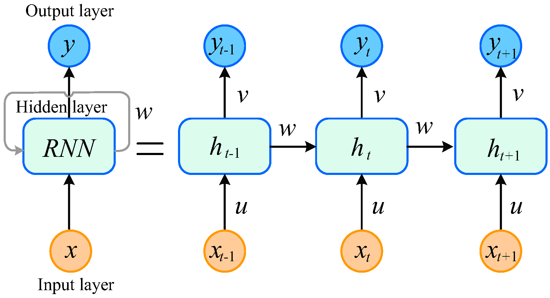
Recurrent neural networks (RNN) were developed in 1986 [35] and are used in handwriting recognition systems. An RNN describes the dynamic behavior of a time series and transmits the state through its own network, so it accepts a wider range of time series inputs. Figure 2 shows the RNN architecture. The relationship between the input and output is expressed as [36]:

$$h_t=w\ast h_{t-1}+u\ast x_t+b$$

(14)

$$y_t=g\left(v\ast h_t\right)$$

(15)

where $x_t$ is the input, $y_t$ is the output, $h_{t-1}$ is the output of the previous hidden layer and $w$, $u$ and $v$ are the parameter vectors.

An RNN is regarded as a neural network that is delivered in the time domain. Each node in the plot is connected through a unidirectional connection to a node in the next successive layer. Every node has a time-varying, real-valued stimulus, and each connection has a real-valued weight that can be modified. Input nodes receive data from outside the network, hidden nodes modify data during the training process from input to output, and output nodes mainly produce network results. An RNN also uses historical prediction information as part of the input. The gradient vanishes for historical data and longer historical information does not affect the prediction results.

3.2.3. LSTM

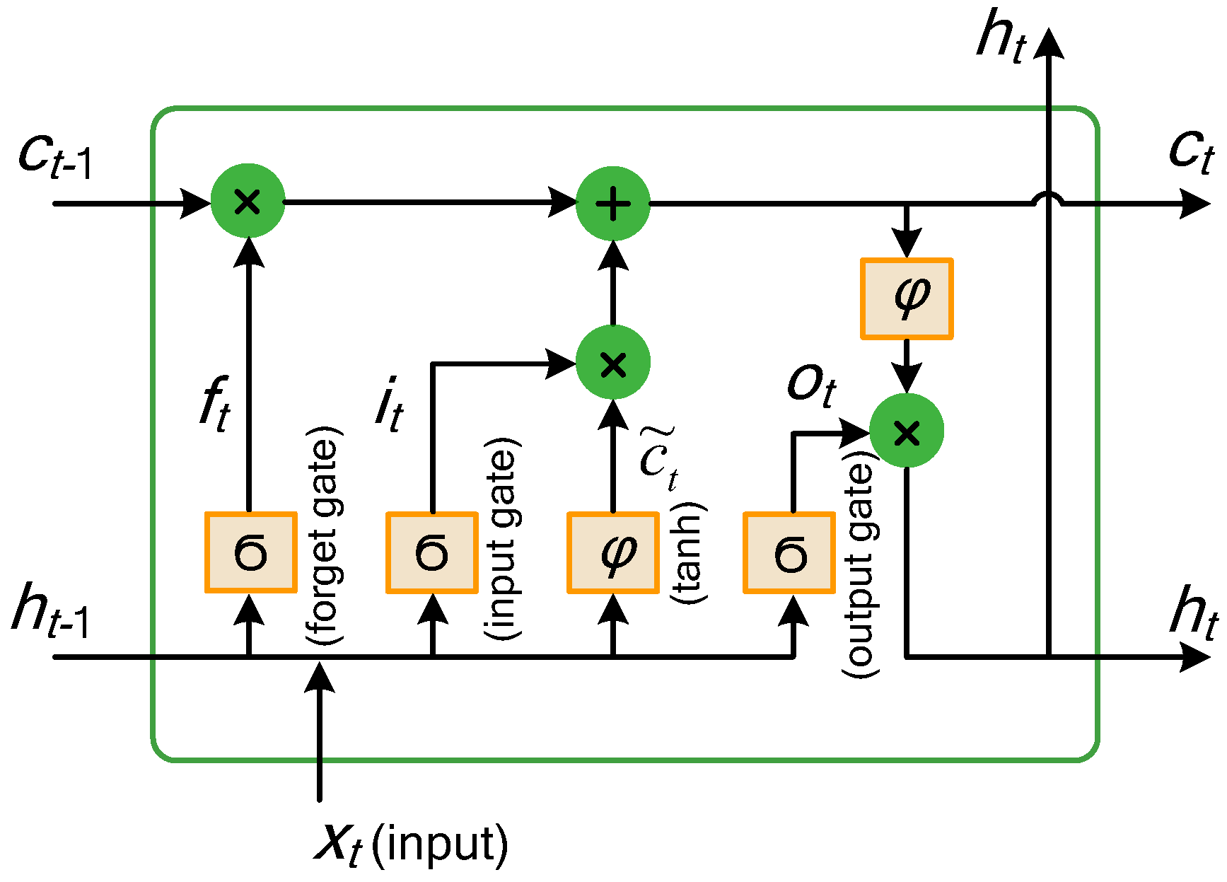
Long short-term memory (LSTM) is a time recurrent neural network that was developed in 1986 [37]. An LSTM is used for processing and predicting important information that features very long intervals and delays in the time series. An LSTM is better suited to longer time series than an RNN. Figure 3 shows the LSTM architecture. The relationship between related nodes is expressed as:

$$f_t=\sigma \left(W_f{x}_t+U_f{h}_{t-1}+b_f\right)$$

(16)

$$i_t=\sigma \left(W_i{x}_t+U_i{h}_{t-1}+b_i\right)$$

(17)

$$o_t=\sigma \left(W_o{x}_t+U_o{h}_{t-1}+b_o\right)$$

(18)

$${\tilde{c}}_t=tanh\left(W_c{x}_t+U_c{h}_{t-1}+b_c\right)$$

(19)

$$c_t=f_t\times c_{t-1}+i_t\times {\tilde{c}}_t$$

(20)

$$h_t=o_t\times \phi \left(c_t\right)$$

(21)

where $x_t$ is the input, $f_t$ is the forget gate, $i_t$ is the input gate, $o_t$ is the output gate, ${\tilde{c}}_t$ is a transfer function, $c_t$ is the cell state, W is an input weight vector, U is an output weight vector for the previous stage, and b is a biased weighted vector.

An LSTM is also an intelligent network unit that can memorize values for an indefinite length of time. The gates in the block determine whether the input is sufficiently important to be remembered and whether it can be output. If the generated value for the forget gate is close to zero, the value that is remembered in the block is forgotten. Similarly, the generated value of the output gate determines whether the output in the block memory can be output.

3.2.4. SVR

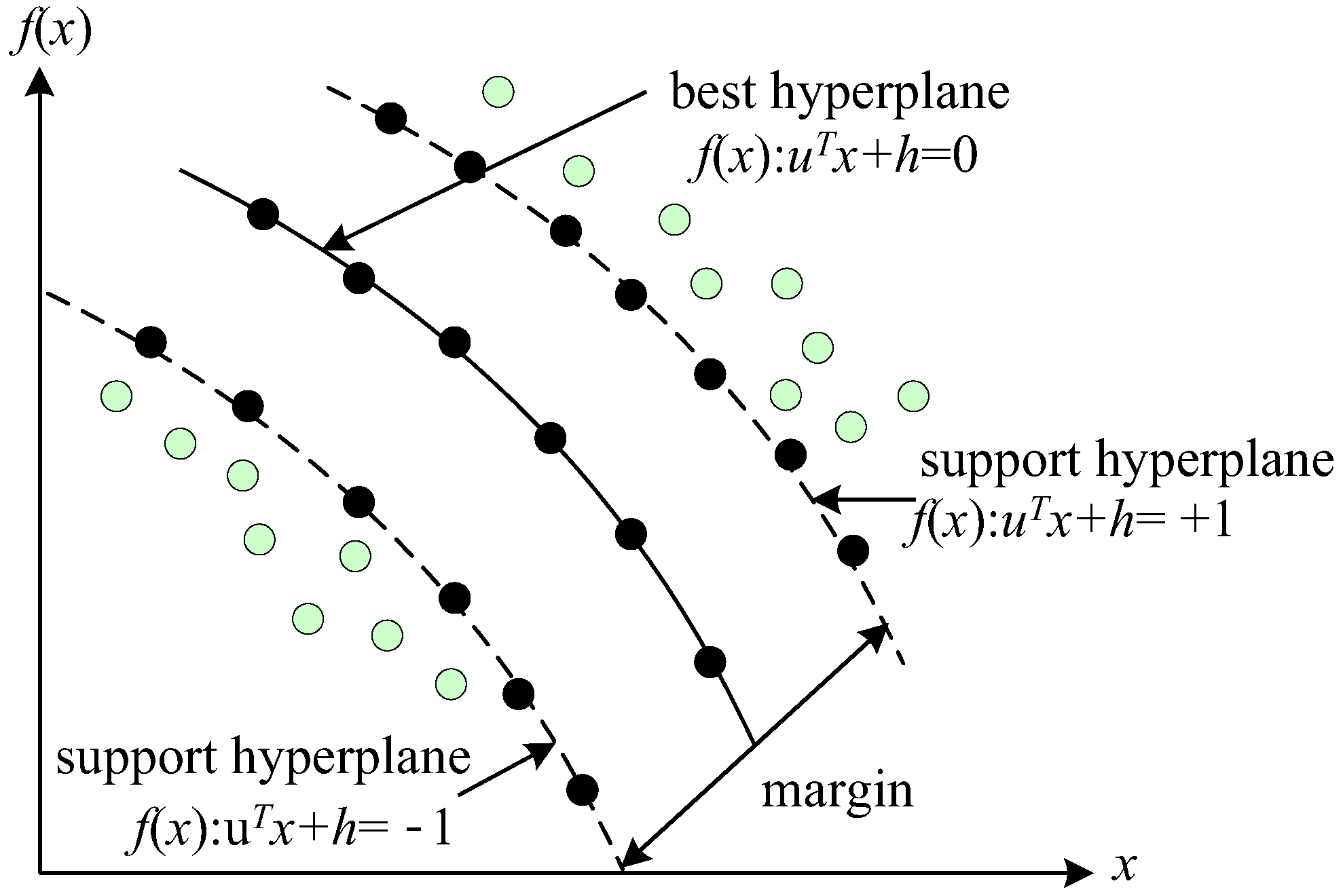
Support Vector Regression (SVR) was proposed by Corter and Vapnik in 1995 [38]. It is used for data classification and regression analysis. An SVR is widely used for image recognition, gene analysis, font recognition, fault diagnosis and load forecasting. Figure 4 shows an SVR hyperplane, which divides the data into high-dimensional spaces, as [39]:

$$\mathrm{Min} f\left(u,\phi \right)= \frac{1}{2}{u}^{T}u+\sigma {\displaystyle \sum }_{k=1}^n{\phi }_k$$

(22)

$$\mathrm{Subject} \mathrm{to} \{\begin{array}{c}{Q}_k\left(u^{T}H\left(x_k\right)+h\right)\ge 1-{\phi }_k\\ {\phi }_k\ge 0 \end{array}$$

(23)

where u is the unit normal vector for the hyperplane, h is the distance from the origin to the hyperplane, n is the number of training data points, ${\phi }_k$ is a swing variable, $\sum {\phi }_k$ is a penalty function, $\sigma$ is the weight of the penalty function, $x_k$ is an input data set, and $H\left(x_k\right)$ is a nonlinear mapping function.

SVR is expressed as a dual optimization problem, as:

$$\mathrm{Max} F_{dual}\left(\mathsf{\lambda }\right)=-\frac{1}{2}{\displaystyle \sum }_{k,l=1}^n{Q}_k{Q}_{l}H{\left(x_k\right)}^{T}H\left(x_l\right){\mathsf{\lambda }}_k{\mathsf{\lambda }}_l+{\displaystyle \sum }_{k=1}^n{\mathsf{\lambda }}_k$$

(24)

$$\mathrm{Subject} \mathrm{to} \{\begin{array}{c}{\displaystyle {\displaystyle \sum }_{k=1}^n}{\mathsf{\lambda }}_k{Q}_k=0 \\ \sigma \ge {\mathsf{\lambda }}_k\ge 0, k=1, 2, \dots , n\end{array}$$

(25)

The term $H{\left(x_k\right)}^{T}H\left(x_l\right)$ in (24) is defined as a kernel function K($x_k$,$x_l$) and must satisfy:

$${\displaystyle \int }K\left(x_k,x_l\right)g\left(x_k\right)g\left(x_l\right)d{x}_{k}d{x}_l\ge 0$$

(26)

where $g\left(x\right)$ is an integrable function. This study uses a radial basis function as the kernel function:

$$\left(x_k,x_l\right)= \exp \left(-\frac{\left|\right|x_k-x_l\left|\right|{}^2}{{\epsilon }^2}\right)$$

(27)

where ε is a dilation parameter.

3.2.5. RFR

The random forest regression (RFR) model is composed of multiple regression trees. Each decision tree is an independent prediction model that is uncorrelated with other trees. The RFR can be used for discrete and continuous data and can also be used for unsupervised clustering learning and outlier detection. Figure 5 shows a schematic diagram of an RFR algorithm. The steps for an RFR algorithm are described as follows [40]:

• n sub-training data sets, $S_1, S_{2, }\dots , S_n,$ are randomly generated from historical data sets.
• CARTs (classification and regression trees) are used to train each set of sub-training data. Some features are extracted and clustered in this step.
• n decision tree models that are used for individual prediction are generated.
• The average of leaf nodes from the training data is treated as the prediction output from each CART.
• The final prediction using an RFR is the average of all prediction outputs of each CART.

Table 1. Comparison of the five single models.

Method	Advantage	Disadvantage
KNN	Implementation is simple and is robust to noisy training data.	Must determine the value of K which may be complex.
RNN	Can accept a wider range of time series inputs.	There is a gradient vanishing phenomenon for longer historical data.
LSTM	Performs better than RNN for longer time series.	Predicts well only for a short time horizon.
SVR	Fits well for a highly nonlinear domain	Modelling is significantly affected by noise.
RFR	Can be used for discrete and continuous data and can also be used for outlier detection.	May converge to a local optimal solution.

shows a brief comparison among the five single models.

3.3. The Optimization Algorithms

Many optimization algorithms can be used to solve weight distribution optimization problems. This study uses swarm-based intelligent methods, such as PSO, SSA and WOA, to determine the weighting value for each single model.

3.3.1. PSO

The particle swarm optimization (PSO) was developed by Kennedy and Eberhart in 1995 [41]. The PSO simulates the behavior of fishes swimming and birds flying as a simplified social system. Each variable (or particle) modifies its position using the previous best position and the best position for the swarm as:

$$\begin{gathered} v_i^d\left(t+1\right)=w{v}_i^d\left(t\right)+r_1\times ran{d}_1\times \left(x_{i, best}\left(t\right)-x_i^d\left(t\right)\right) \\ +r_2\times ran{d}_2\times \left(s_{best}\left(t\right)-x_i^d\left(t\right)\right) \end{gathered}$$

(28)

$$x_i^d\left(t+1\right)=x_i^d\left(t\right)+v_i^d\left(t+1\right)$$

(29)

where $v_i^d\left(t+1\right)$ is the velocity of the ith particle at the (t + 1)th iteration, i = 1, 2, …, P, P is the population size and d = 1, 2, …, D, D is the dimension of the variable, $w$ is the weighting value, $v_i^d\left(t\right)$ is the previous velocity, $r_1$ and $r_2$ are the parameters for self-cognition and the swarm, respectively, $ran{d}_1$ and $ran{d}_{2 }$ are random numbers with a uniform distribution, $x_{i,best}\left(t\right)$ is the best position for the ith particle at the tth iteration, $s_{best}\left(t\right)$ is the best position for the swarm at the tth iteration, $x_i^d\left(t+1\right)$ is the position of the ith particle at the (t + 1)th iteration and $x_i^d\left(t\right)$ is the previous position.

3.3.2. SSA

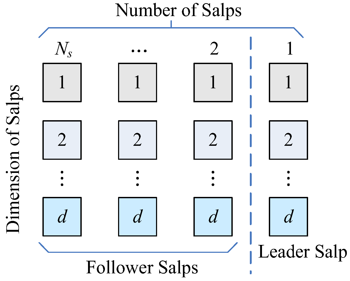
The salp swarm algorithm (SSA) was developed by Mirjalili et al. in 2017 [42]. It simulates the group activities of a salp swarm chain. SSA performs exploration and exploitation during the optimization process. During the foraging process, salps naturally form a group chain structure, as shown in Figure 6, are either leader salp or follower salps. The leader salp swims ahead and guides the whole group forward and updates the swimming direction depending on the position of the food. The other salps are called follower salps, and they update their positions depending on the position of the leader salp. The leader salp updates its position as:

$$x_1^j\left(t+1\right)=\{\begin{array}{c}{x}_{best}^j\left(t\right)+c_1\left(\left(x_{1, max}^j-x_{1, min}^j\right)\times c_2+x_{1, min}^j\right), c_3\le 0.5 \\ x_{best}^j\left(t\right)-c_1\left(\left(x_{1, max}^j-x_{1, min}^j\right)\times c_2+x_{1, min}^j\right), c_3>0.5\end{array}$$

(30)

where $x_1^j\left(t+1\right)$ is the position of the leader salp for the ith particle at the (t + 1)th iteration, $x_{best}^j$ is the best position for the jth particle, $x_{1, min}^j$ and $x_{1, max}^j$ are the lower and upper limits for the jth variable, the parameters $c_2$ and $c_3$ are uniform random numbers and $c_1$ maintains a balance between exploration and exploitation and is expressed as:

$$c_1=2exp\left(-{\left(\frac{4t}{t_m}\right)}^2\right)$$

(31)

where $t$ is the current iteration and $t_m$ is the maximum number of iterations.

When the position of the leader salp is updated, the positions of the follower salps are updated as:

$$x_i^j\left(t+1\right)=\frac{1}{2}\left(x_i^j\left(t\right)+x_{i-1}^j\left(t\right)\right)$$

(32)

$$x_i^j\left(t\right)=\frac{1}{2}a{t}^2+v_{0}t$$

(33)

where $i=2, 3, \dots , N_s$, $N_s$ is the number of follower salps,$v_0$ is the initial velocity and $a$ is the acceleration.

3.3.3. WOA

The whale optimization algorithm (WOA) was developed by Mirjalili and Lewis in 2016 [43]. It simulates the fishing strategy of the humpback whale and uses encircling prey, bubble net attack, and search for prey strategies to fish, as described in the following:

• Encircling prey

Humpback whales encircle prey when they find the location of the prey as follows:

$$\overrightarrow{P}\left(t+1\right)={\overrightarrow{P}}_{best}\left(t\right)-\overrightarrow{B}·\overrightarrow{C}$$

(34)

$$\overrightarrow{C}=\left|\overrightarrow{E}·{\overrightarrow{P}}_{best}\left(t\right)-\overrightarrow{P}\left(t\right)\right|$$

(35)

where $\overrightarrow{P}\left(t\right)$ is the current position vector, ${\overrightarrow{P}}_{best}\left(t\right)$ is the previous best position vector, $\overrightarrow{B} \left(=2\overrightarrow{b}·\overrightarrow{r}-\overrightarrow{b}\right),$ $\overrightarrow{C}$ and $\overrightarrow{E}\left(=2·\overrightarrow{r}\right)$ are coefficient vectors,$\overrightarrow{r}$ is a uniform random vector, $\overrightarrow{b}$ gradually decreases from 2 to 0, so $\overrightarrow{B}$ is between 0 and 1, and ”$·$” represents an inner product operation.

• Bubble net attack

Surrounding the prey is the most common attack strategy by humpback whales. It also hunts prey using the bubble net attack as:

$$\overrightarrow{P}\left(t+1\right)=\{\begin{array}{cc}{\overrightarrow{P}}_{best}\left(\mathrm{t}\right)-\overrightarrow{B}·\overrightarrow{C},\hfill & if p<0.5\hfill \\ \left|{\overrightarrow{P}}_{best}\left(t\right)-\overrightarrow{P}\left(t\right)\right|·e^{el}·\cos \left(2\pi l\right)+{\overrightarrow{P}}_{best}\left(t\right),\hfill & if p\ge 0.5\hfill \end{array}$$

(36)

where $\left|{\overrightarrow{P}}_{best}\left(t\right)-\overrightarrow{P}\left(t\right)\right|$ is the distance between the humpback whales and the prey, $e$ is a constant that defines the shape of the logarithmic spiral and l and $p$ are random numbers between 0 and 1.

• Search for prey

To increase exploration, humpback whales use $\left|B\right|>1$ to avoid falling into local optima as:

$$\overrightarrow{P}\left(t+1\right)={\overrightarrow{P}}_{rand}-\overrightarrow{B}·\overrightarrow{C}$$

(37)

$$\overrightarrow{C}=\left|\overrightarrow{E}·{\overrightarrow{P}}_{rand}-\overrightarrow{P}\left(t\right)\right|$$

(38)

where ${\overrightarrow{P}}_{rand}$ is randomly selected from the swarm.

3.4. The Scheme for Optimizing Weight Distribution

In contrast to a traditional stacking method, the proposed method uses an optimization algorithm to determine the weight distribution for each single model. A preliminary forecast is generated from every single model. The final forecast is produced by combining the weight output of each single model. The steps for using an optimization algorithm to determine the weight for each single model are described in the following:

Step 1: The initial position of each particle is randomly generated as:

$$x_{i,j}\left(0\right)=x_{i,min}+rand\times \left(x_{i,max}-x_{i,min}\right), i=1, 2, \dots , S, j=1, 2, \dots , P$$

(39)

where $x_{i,j}\left(0\right)$ is the initial position of the ith variable of the jth feasible solution, $x_{i,max}$ and $x_{i,min}$ are the maximum and minimum positions, respectively, $rand$∈[0,1] is the value of the uniform distribution function, S is the number of variables, and P is the number of feasible solutions for the group. The position of the jth feasible solution is expressed as:

$$x_j=\left[w_{1,h}, w_{2,h},\dots , w_{5,h}\right], h=1, 2, \dots , 24, j=1, 2, \dots , P$$

(40)

$${\displaystyle \sum }_{i=1}^5{w}_{i,h}=1, w_{i,h}\ge 0$$

(41)

where $w_{i,h}$ is the weight of the ith prediction model at the hth hour. This study generates a feasible solution for the first hour (i.e., $x_j=[w_{1,1}, w_{2,1},\dots , w_{5,1}]$, $j=1, 2, \dots , P$). After optimization, the weight distribution for each single model for the remaining hours is optimized successively.

Step 2: The fitness value for each initial feasible solution is calculated, and the position of the best initial feasible solution is recorded. The fitness value for the jth feasible solution at the hth hour is expressed as:

$$F_{j,h}={\displaystyle \sum }_{i=1}^5{\left({\widehat{\mathit{Y}}}_{i,h}\times w_{i,h}-{\mathit{Y}}_{i,h}\right)}^2, h=1, 2, \dots , 24, j=1, 2, \dots , P$$

(42)

where ${\widehat{\mathit{Y}}}_{i,h}=\left[{\widehat{Y}}_1,{\widehat{Y}}_2, \dots , {\widehat{Y}}_N\right]$ is the estimated value of the training data for the jth feasible solution at the hth hour, and N is the number of training data points. ${\mathit{Y}}_{i,h}=\left[Y_1,Y_2, \dots ,Y_N\right]$ is the actual value of the training data for the jth feasible solution at the hth hour.

Step 3: A position updating strategy is used in this step.

• PSO: use (28) and (29) to modify velocity and position;
• SSA: use (30) and (32) to update the positions of the leader salp and the follower salps, respectively;
• WOA: use encircling prey, bubble net attack, and search for prey strategies to update the position of the humpback whales as shown in (35) to (37).

Step 4: The fitness value for each updated position is calculated using (42). The position with the best fitness value is selected as the next generation.

Step 5: If the maximum number of iterations is achieved, the method determines whether the 24 h weighting optimization is complete. If it is, the optimal 24 h weighting solution is output; if none of the above conditions are met, steps 3–5 are repeated.

4. Numerical Results

4.1. Data Pre-Processing

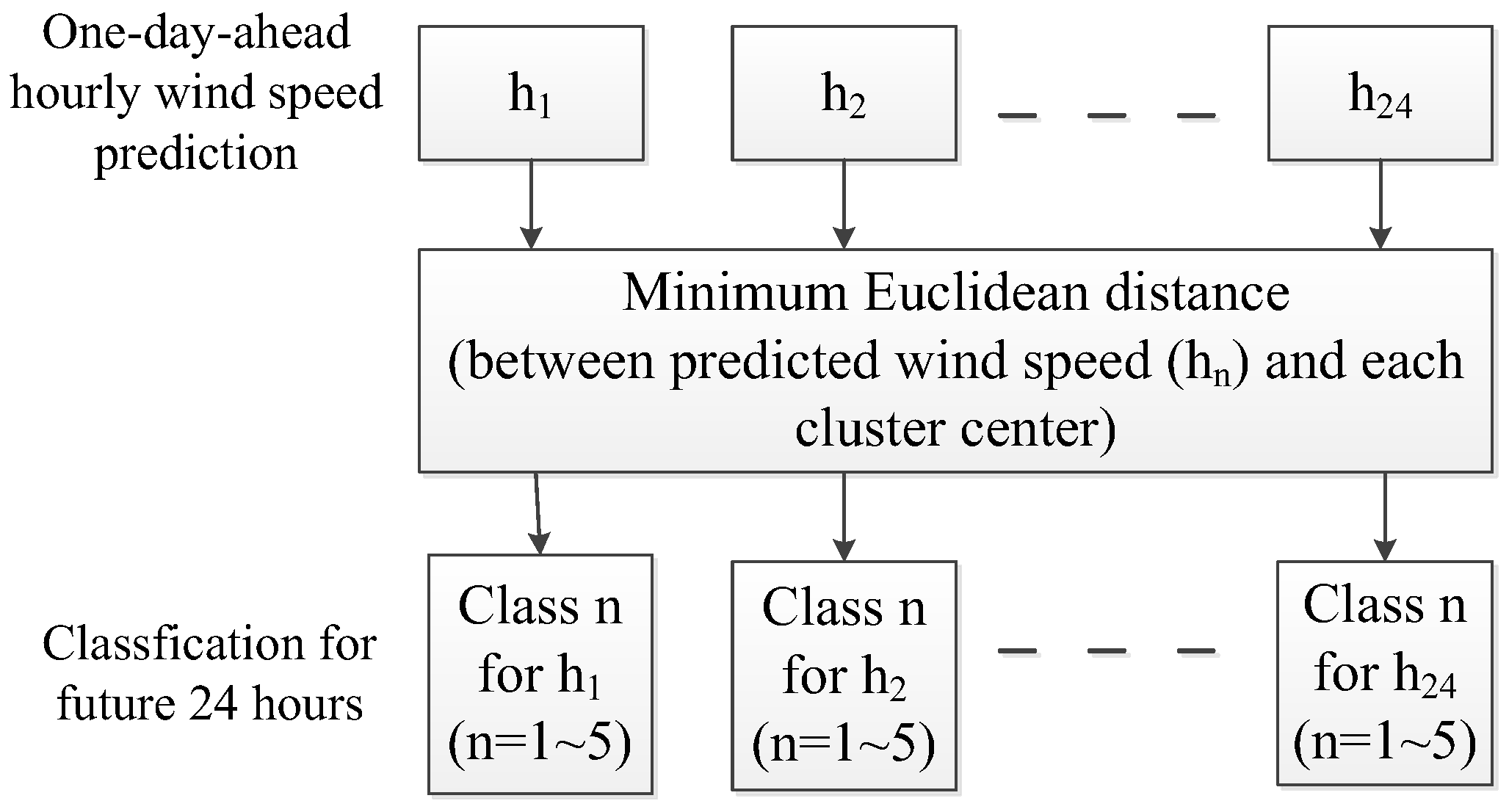
The proposed method was used for a 3.6 MW wind turbine power generation system that is located in Changhua, Taiwan. Data was collected from December 2019 to September 2021, to give a total of 11,527 hourly data points when outliers or missing data are eliminated. From the 11,527-hourly data points, 10,951 data points are used to construct and validate five single models and the remaining 576 data points (for a total of 24 days, distributed over each month) are used for testing. The data includes wind power, wind speed, and wind direction. Figure 7 shows the schematic diagram of class selection for future prediction points. If the future wind speed prediction at the first hour is ${\mathrm{h}}_1$, calculate the Euclidean distance between ${\mathrm{h}}_1$ and each cluster center (a total of five cluster centers). The class with the shortest Euclidean distance is chosen for ${\mathrm{h}}_1$. Five single models then use the same class of prediction model that is constructed in the training stage to generate a preliminary forecast.

The wind speed data is measured at the hub height of 10 m. In order to ensure that wind speed data for the wind turbine at a height of 67 m can be used, the following conversion formula is used [44]:

$$\frac{v\left(z_2\right)}{v\left(z_1\right)}={\left(\frac{z_2}{z_1}\right)}^{\alpha }$$

(43)

where $z_1=10 \left(m\right)$, $z_2=67 \left(m\right)$, $\alpha$ is the surface friction coefficient, which value is obtained by experiment. The $\alpha$ value in the smooth area is low, and the α value in the rough blocking area is high. Generally, $\alpha$ has a value between 0.1 and 0.4. For this study, $\alpha$ is 0.2. The program was run on a Windows 11 PC using Python software.

Figure 8 shows the curves for wind power data before and after pre-processing. A Pearson correlation coefficient is used to determine the effects of wind speed and wind direction on wind power. The k-means method is used to classify historical wind power data into several categories. Figure 9 shows an elbow curve for the collected wind power data. The sum of square error (SSE $={\displaystyle \sum }_{i=1}^n{\left(y_i-{\widehat{y}}_i\right)}^2$) decreases as the number of clusters increases. When the number of clusters is greater than 5, SSE decreases slowly. As shown in Figure 10, the historical wind power data are then divided into five categories such as breeze (class 1), moderate wind (class 2), cool wind (class 3), strong wind (class 4), and powerful wind (class 5). To illustrate the impact of data classification on prediction accuracy, five single models are also used to establish the individual prediction models without classifying the data.

Table 2. Prediction error of data before and after classification.

Data Type	KNN	RNN	LSTM	SVR	RFR
Before classification	2.7151	2.6857	2.6906	3.3102	2.7350
After classification (five categories)	2.2519	2.3386	2.3340	2.2763	2.2951
Error reduction	17.0601%	12.9240%	13.2535%	31.2338%	16.0841%

shows the prediction error of data before and after classification. The data after classifying into five categories increase prediction accuracy by 12% to 31%.

Table 3. Pearson correlation coefficient values between weather variables and wind power.

	Before Pre-Processing			After Pre-Processing
Variable	Wind Power	Wind Speed	Wind Direction	Wind Power	Wind Speed	Wind Direction
Wind power	1.00	0.90	−0.52	1.00	0.96	−0.51
Wind speed	0.90	1.00	−0.45	0.96	1.00	−0.49
Wind direction	−0.52	−0.45	1.00	−0.51	−0.49	1.00

shows the correlation coefficient values before and after pre-processing. After data pre-processing, the correlation coefficient values between weather variables and wind power are greater. As shown in this table, wind speed has a great effect on wind power. There is a small mutual correlation between wind speed and wind direction. In this study, the wind speed and wind direction are used as explanatory variables to establish each single prediction model.

Table 4. The number of data points that are used for every category.

Category	Training Data	Validation Data	Testing Data
Class 1 (breeze)	3838	427	129
Class 2 (moderate wind)	1792	200	161
Class 3 (cool wind)	1059	118	139
Class 4 (strong wind)	976	109	107
Class 5 (powerful wind)	2208	224	40
Total	9873	1078	576

shows the number of data points for every category that are used for training, validation, and testing.

Table 5. Parameter settings for every single model.

Method	Parameter	Class 1	Class 2	Class 3	Class 4	Class 5
KNN	No. of K	10	5	5	5	5
	Distance	Euclidean	Euclidean	Euclidean	Euclidean	Euclidean
RNN	No. of 1st layer neuron	12	12	12	12	12
	Activation fun. of 1st layer	Relu 1	Relu	Relu	Relu	Relu
	No. of 2nd layer neuron	6	6	6	6	None
	Activation fun. 2 of 2nd layer	Relu	Relu	Relu	Relu	None
	Activation fun. of output	Sigmoid	Sigmoid	Sigmoid	Sigmoid	Sigmoid
LSTM	No. of 1st layer neuron	12	12	12	12	12
	Activation fun. of 1st layer	Relu	Relu	Relu	Relu	Relu
	No. of 2nd layer neuron	6	6	6	6	None
	Activation fun. of 2nd layer	Relu	Relu	Relu	Relu	None
	Activation fun. of output	Sigmoid	Sigmoid	Sigmoid	Sigmoid	Sigmoid
SVR	Kernel function	RBF 3	RBF	RBF	RBF	RBF
	Dilation parameter (ε)	0.1	0.1	0.1	0.1	0.1
	Weight of penalty ($\sigma$)	1	1	1	1	1
RFR	No. of tree	100	100	100	100	100
	Loss function	MSE	MSE	MSE	MSE	MSE

¹: Rectified linear unit; ²: activation function; ³: radial basis function.

shows the parameter settings for every single model. To determine the forecasting accuracy, the mean relative error (MRE) is used as:

$$\mathrm{MRE}=\frac{1}{N}{\displaystyle \sum }_{i=1}^N\left|\frac{y_i-{\widehat{y}}_i}{y_{cap}}\right|\times 100\%$$

(44)

where $y_i$ is the ith actual value, ${\widehat{y}}_i$ is the ith estimated value, $y_{cap}$ is the capacity to generate wind power, and N is the number of estimation points.

4.2. Forecasting Results

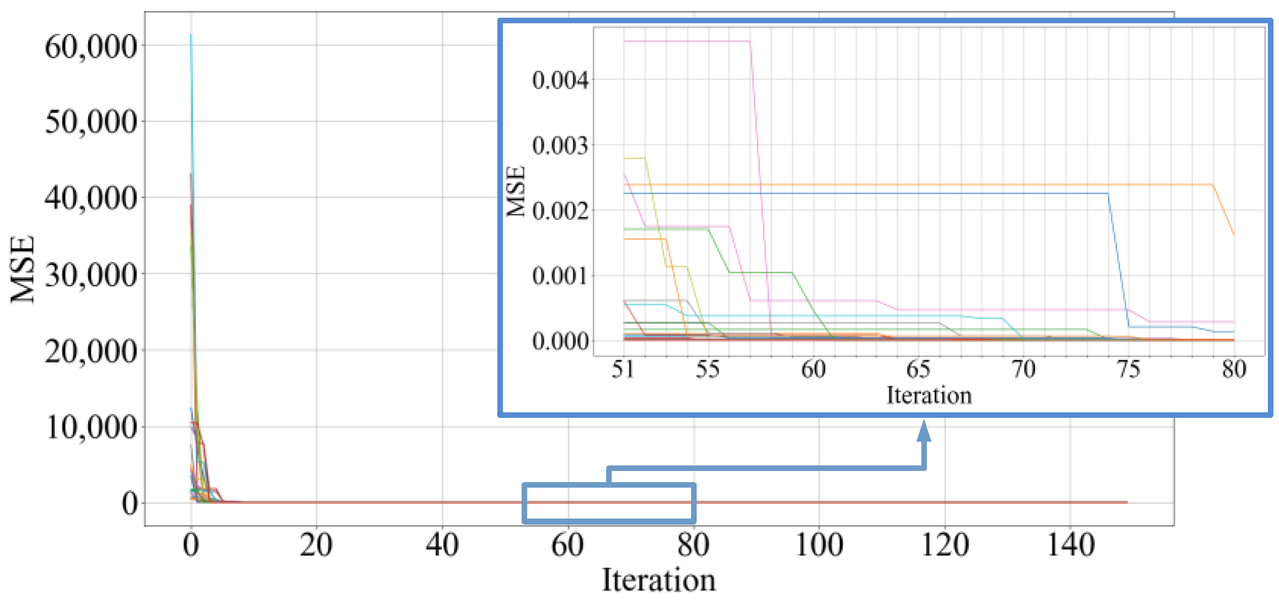
Five machine learning methods (KNN, RNN, LSTM, SVR and RFR) are used to establish individual prediction models for each grade of wind, in order to generate a preliminary forecast. The inputs for each model are wind speed and wind direction, and the output is wind power.

Table 6. Validation results (MRE%) for every single prediction model.

Model	Class 1	Class 2	Class 3	Class 4	Class 5	Average
KNN	0.9012	2.1888	2.7964	2.6028	1.6672	2.0313
RNN	0.8925	2.1342	2.7431	2.6230	1.6232	2.0032
LSTM	0.8641	2.1831	2.6830	2.7327	1.6071	2.0140
SVR	0.9426	2.2965	2.7532	2.9795	1.8333	2.1610
RFR	0.9401	2.3134	3.1120	3.3632	1.6263	2.2710

shows the validation results (MRE%) for every single prediction model. Every single model produces good predictions using the validation data, which demonstrates that those models do not overfit and can be used for preliminary prediction.

Table 7. Parameter settings for every optimization algorithm.

PSO		SSA		WOA
Parameter	Value	Parameter	Value	Parameter	Value
Population size	40	Population size	40	Population size	40
Max. iteration	150	Max. iteration	150	Max. iteration	150
Weight (w)	0.8	Variable ($c_1$)	$2\to 0$	Random ($l, p, r)$	all in (0, 1)
self-cognition ($r_1$)	0.5	Random ($c_2$)	(0, 1)	Variable ($b$)	$2\to 0$
Swarm ($r_2$)	0.5	Random ($c_3$)	(0, 1)	Constant ($e$)	1

shows the parameter settings for every optimization algorithm. These parameters are tuned by experiment. Figure 11, Figure 12 and Figure 13, respectively, show the optimization curves for PSO, SSA and WOA methods. The mean squired error (MSE) is used to evaluate the convergence characteristic as:

$$\mathrm{MSE}=\frac{1}{N}{\displaystyle \sum }_{i=1}^N{\left(y_i-{\widehat{y}}_i\right)}^2$$

(45)

Each plot contains 24 (hourly) optimization curves. In order to easily observe the convergence characteristics, the curves for the 51st to 80th iterations are magnified. The respective convergence average MSE values for PSO, SSA, and WOA are 8.89 × 10⁻⁸, 1.10 × 10⁻¹⁰ and 1.53 × 10⁻⁶. The convergence time for 24 h for the PSO is 101.08 (s) and the SSA and WOA, respectively, require 113.32 (s) and 134.08 (s) after 150 iterations.

Table 8. The respective weights for each individual model using a WOA for 24 h.

Hour	KNN	RNN	LSTM	SVR	RFR
1	0.2262	0.0627	0.2352	0.2182	0.2576
2	0.0898	0.3736	0.3102	0.0763	0.1502
3	0.4501	0.3193	0.1829	0.0477	0.0000
4	0.0691	0.0242	0.1575	0.4971	0.2521
5	0.0445	0.6718	0.1202	0.0701	0.0934
6	0.1224	0.0753	0.2089	0.3023	0.2911
7	0.1389	0.1487	0.4855	0.0893	0.1376
8	0.0000	0.0002	0.6560	0.3438	0.0000
9	0.0404	0.4588	0.0858	0.0314	0.3835
10	0.5613	0.4387	0.0000	0.0000	0.0000
11	0.0000	0.2994	0.3873	0.0000	0.3133
12	0.0777	0.0257	0.6407	0.0496	0.2063
13	0.6795	0.0000	0.0000	0.2312	0.0893
14	0.1720	0.1391	0.2133	0.3892	0.0864
15	0.0880	0.0721	0.2099	0.0186	0.6114
16	0.0000	0.2586	0.6494	0.0202	0.0718
17	0.1299	0.1748	0.0034	0.3020	0.3900
18	0.1215	0.1951	0.2336	0.2133	0.2364
19	0.0293	0.0499	0.3308	0.2019	0.3881
20	0.6182	0.0020	0.3797	0.0000	0.0000
21	0.2606	0.5113	0.0000	0.2281	0.0000
22	0.5118	0.2357	0.0427	0.0959	0.1138
23	0.0040	0.2044	0.2736	0.2961	0.2219
24	0.0846	0.6015	0.1835	0.0008	0.1296

shows the respective weights for each individual model for the 24 h using the WOA method. A weight of zero signifies a prediction model that has no effect on the output. Similar weight matrices are generated using the PSO and SSA methods.

The Taiwanese Central Weather Bureau (TCWB) only provides 3-h-ahead wind speed predictions, so the data is not suitable for one-day-ahead hourly wind power forecasting. Solcast is a forecasting platform that offers meteorological predictions including temperature, wind speed, wind direction, and humidity at different resolutions, as long as the latitude and longitude locations are provided [45]. However, the wind speed prediction that is provided by Solcast features a 16.31% forecasting error, compared to the actual measured wind speed. A correction model to increase prediction accuracy for wind speed is then constructed. The RFR model that gives better results than the other single models for the Solcast forecasting data is used to correct the Solcast predictions. During training, the inputs are the Solcast predictions for wind speed and wind direction and the output is the actual measured wind speed. After training, the forecasting error for wind speed is reduced from 16.31% to 4.56%. The RFR model for wind speed correction is then used for one-day-ahead hourly wind speed prediction based on the Solcast forecasting data.

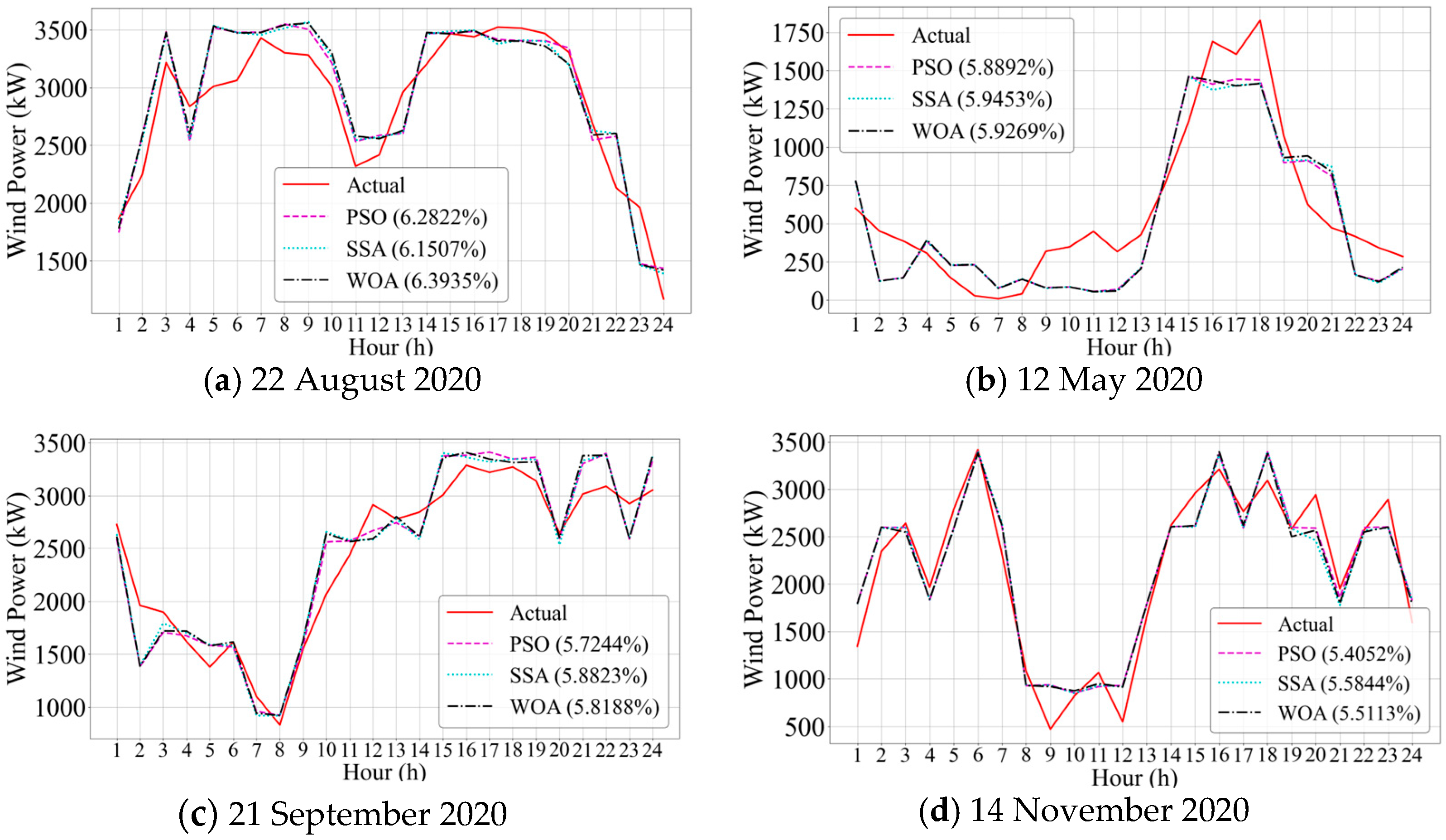
Figure 14 shows the curves for the forecasting results for four different testing days using the PSO, SSA and WOA methods.

Table 9. Forecasting errors for single and ensemble models using proposed corrected data.

Date\Model	Single Model					Ensemble Model
	KNN	RNN	LSTM	SVR	RFR	PSO	SSA	WOA
13 January 2020	5.7471	6.1680	6.1432	6.2540	6.1402	6.1905	6.1642	6.0919
21 January 2020	6.6185	6.1772	6.1612	6.4455	6.2487	6.1779	6.2325	6.2194
21 February 2020	4.5511	4.7681	4.8243	4.7534	4.8212	4.7488	4.7000	4.7045
27 February 2020	6.7134	6.5302	6.5243	6.1571	6.5253	6.2822	6.1507	6.3935
15 March 2020	7.7719	7.59 23	7.4994	7.6335	7.9271	7.4691	7.5110	7.5170
24 March 2020	6.3340	5.9949	5.8390	5.9757	5.7736	5.8768	5.9384	5.8841
8 April 2020	6.6817	6.4063	6.3512	6.2187	6.0752	6.3104	6.3134	6.3361
27 April 2020	5.5673	5.4448	5.5617	5.5234	5.6947	5.4364	5.2975	5.2275
12 May 2020	6.3354	5.9980	6.0030	5.9687	5.9309	5.8892	5.9453	5.9269
23 May 2020	6.7737	6.5872	6.7452	6.8120	7.0053	6.7576	6.6027	6.6950
6 June 2020	6.0505	6.1892	6.2511	6.3421	6.6123	6.3614	6.3140	6.3036
9 June 2020	3.4923	3.3150	3.4267	3.3293	3.4050	3.4161	3.4172	3.4716
9 July 2020	5.2505	6.0029	6.0191	6.4007	6.3822	6.2873	6.2053	6.2191
16 July 2020	4.9644	5.7943	5.7140	6.2564	6.6771	6.1760	6.2155	6.1706
13 August 2020	2.8326	2.8658	2.9068	2.7724	2.8732	2.8256	2.8017	2.8533
26 August 2020	5.6586	5.4043	5.4455	5.2020	5.6817	5.3389	5.2997	5.5734
21 September 2020	5.3698	5.9006	5.9325	5.5107	5.7705	5.7244	5.8823	5.8188
25 September 2020	7.5417	7.2010	7.1295	7.2682	6.6625	7.0298	7.0801	7.0778
9 October 2020	6.5067	5.5500	5.7223	5.7209	6.6122	5.5757	5.7450	5.6051
26 October 2020	6.0354	5.6619	5.7231	5.7282	5.6856	5.7075	5.6588	5.5234
14 November 2020	5.7571	5.5642	5.6268	5.6021	5.4525	5.4052	5.5844	5.5113
25 November 2020	5.6828	5.8060	5.7580	5.7667	5.9269	5.7826	5.7632	5.8795
23 December 2020	5.6999	5.5851	5.6177	5.6146	5.8831	5.6308	5.5530	5.6166
29 December 2020	5.4818	5.2597	5.3664	5.2853	5.6575	5.3659	5.2861	5.1703
Average	5.8091	5.7423	5.7622	5.7726	5.8927	5.7403	5.7359	5.7413

shows the forecasting results for single and ensemble models using the corrected wind speed data. For the 24 test datasets, the respective average MRE value for KNN, RNN, LSTM, SVR, the ensemble-based PSO, SSA, and WOA is 5.8091%, 5.7423%, 5.7622%, 5.7726%, 5.8937%, 5.7403%, 5.7359% and 5.7413%. The optimized ensemble methods give a more accurate forecast than the single models.

Table 10. Number of maximum and minimum MREs for single and ensemble models.

	Single Model					Ensemble Model
Model	KNN	RNN	LSTM	SVR	RFR	PSO	SSA	WOA
No. of Maximum MRE	9	0	1	2	12	0	0	0
No. of Minimum MRE	7	3	2	2	3	2	2	3

shows the number of maximum and minimum MRE values for single and ensemble models. In terms of the number of maximum MRE, RFR gives a less accurate forecast than the other single and ensemble models. The RNN model and the ensemble models do not produce the worst prediction for all of the test datasets. In terms of the number of minimum MRE values, KNN gives an accurate forecast for seven test datasets; RNN, RFR, and ensemble WOA produce an accurate forecast for three test datasets.

Table 11. Forecasting results for average MRE using actual data, Solcast prediction data and corrected data.

Testing Data (Wind Speed and Wind Direction)	Single Model					Ensemble Model
	KNN	RNN	LSTM	SVR	RFR	PSO	SSA	WOA
Actual measured data	2.2519	2.3386	2.3340	2.2763	2.2951	2.2812	2.2779	2.2304
Solcast prediction data	8.8783	8.4612	8.7452	6.4671	6.9529	7.5546	7.7721	7.5512
Solcast prediction data using $10\%$ random error	7.6128	7.9735	8.0849	6.5136	7.1837	7.3545	7.2809	7.3137
Prediction data using proposed correction model	5.8091	5.7423	5.7622	5.7726	5.8927	5.7403	5.7359	5.7413

shows the forecasting results for average MRE using actual data, Solcast forecasting data, Solcast forecasting data with $10\%$ random error, and the forecasting data after correction. If the actual measured wind speed and wind direction are used, the optimized ensemble models give a more accurate forecast than the single models, except for the KNN model. If predicted wind speed and wind direction data that are provided by the Solcast are used, SVR gives a more accurate result than all other models. The optimized ensemble models also allow accurate forecasts.

To simulate the inaccuracy for weather forecasts, a random error with normal distribution is added to the Solcast forecasting data [46]. During the experiment, the random errors for $10\%$, $20\%$, $30\%$, and $40\%$ are used for the test. A random error of $10\%$ that allows a more accurate forecast is used to correct the Solcast forecasting data. As shown in Table 11, the forecasting results give a slightly better result than the results using Solcast prediction data. If the proposed wind speed correction model is used, the wind power forecasting errors reduce about 2~3% MRE value for each single and ensemble model. This case is mainly used to represent an optimized ensemble method that can be better than a single prediction method.

Table 12. Comparison between the proposed SBI and the other ensemble methods using LASSO and ridge regressions.

Testing Data (Wind Speed and Wind Direction)	Ensemble Model
Prediction data using proposed correction model	LASSO [25]	Ridge [27]	PSO	SSA	WOA
	5.7509	5.7572	5.7403	5.7359	5.7413

compares the SBI methods with other ensemble methods using LASSO [25] and ridge regression [27], which use a Bayesian optimization algorithm to determine the weight distribution for each single model. This case is mainly used to highlight the SBI methods such as PSO, SSA, and WOA, which give more accurate forecasts than LASSO and ridge regression methods.

4.3. Discussion

An SBI method that is used to optimize the weights distribution for each single model gives a more accurate wind power forecast than the single and ensemble prediction models. The forecasting results allow the following observations:

• Five single models, including KNN, RNN, LSTM, SVR, and RFR are used to produce a preliminary forecast. More machine learning models can be used as a single model to avoid overestimation and to increase the forecasting accuracy.
• As shown in Table 9 and Table 10, the optimized ensemble models do not give the best forecast on every test dataset, but no maximum MRE value is produced using the ensemble models.
• There is a high correlation between wind speed and wind power data. The accuracy of the wind speed prediction significantly affects the wind power forecast. Compared to the Solcast prediction results, a decrease of about 2~3% MRE value is obtained by using the proposed wind speed correction model.
• This study uses an RFR model to decrease the wind speed prediction error from 16.31% to 4.56%. A more accurate prediction method can be used to increase the forecasting accuracy of wind speed, such as those of previous studies in [5,6,7,8,9,10,11,12].
• A Bayesian optimization algorithm is used to determine the weight distribution for each single model by the LASSO and ridge regression methods. The proposed method uses SBI algorithms to optimize the weight distribution and allows a more accurate prediction.

5. Conclusions

An optimized ensemble model for one-day-ahead hourly wind power forecasting is proposed to increase the forecasting accuracy for single prediction models. The proposed method first divides historical wind power data into five different categories. Five single models, including KNN, RNN, LSTM, SVR, and RFR, are used to establish individual prediction models for each category of data, in order to produce a preliminary forecast. The final prediction is generated using a swarm-based intelligent tool to determine the weight distribution for each single model. The wind speed prediction that is provided by a forecasting platform features a 16.31% forecasting error. An RFR model is used to reduce the wind speed prediction error from 16.31% to 4.56%. Testing with a 3.6 MW wind power generation system shows that the optimized ensemble method gives a more accurate forecast than the single models. The ensemble models do not produce the worst prediction for all test datasets. Using the proposed wind speed correction model, the wind power forecasting error is reduced by 2~3% MRE value for each single and ensemble model. The proposed method also allows more accurate forecasting than the LASSO and ridge regression methods. Future studies will dynamically update the weight value for each single prediction model using new wind power data, in order to increase forecasting accuracy.

References

1. Shobana, S.; Gnanavel, B.K. Optimised Coordinated Control of Hybrid AC/DC Microgrids along PV-Wind-Battery: A Hybrid Based Model. Int. J. Bio-Inspired Comput. 2022, 20, 193–208. [Google Scholar] [CrossRef]
2. Sun, X.; Yang, X.; Cai, J.; Jiang, X. Transient Protection Schemes for Transmission Lines Used in Offshore Wind Farm: A State-of-the-Art Review. Front. Energy Res. 2022, 10, 741. [Google Scholar] [CrossRef]
3. Kou, L.; Li, Y.; Zhang, F.; Gong, X.; Hu, Y.; Yuan, Q.; Ke, W. Review on Monitoring, Operation and Maintenance of Smart Offshore Wind Farms. Sensors 2022, 22, 2822. [Google Scholar] [CrossRef]
4. Piotrowski, P.; Rutyna, I.; Baczyński, D.; Kopyt, M. Evaluation Metrics for Wind Power Forecasts: A Comprehensive Review and Statistical Analysis of Errors. Energies 2023, 15, 9657. [Google Scholar] [CrossRef]
5. Li, M.; Yang, M.; Yu, Y.; Lee, W.J. A Wind Speed Correction Method Based on Modified Hidden Markov Model for Enhancing Wind Power Forecast. IEEE Trans. Ind. Appl. 2022, 58, 656–666. [Google Scholar] [CrossRef]
6. Zheng, Z.; Wang, L.; Yang, L.; Zhang, Z. Generative Probabilistic Wind Speed Forecasting: A Variational Recurrent Autoencoder Based Method. IEEE Trans. Power Syst. 2022, 37, 1386–1398. [Google Scholar] [CrossRef]
7. Mogos, A.S.; Salauddin, M.; Liang, X.; Chung, C.Y. An Effective Very Short-Term Wind Speed Prediction Approach Using Multiple Regression Models. IEEE Can. J. Electr. Comput. Eng. 2022, 45, 242–253. [Google Scholar] [CrossRef]
8. Sun, S.; Qiao, H.; Wei, Y.; Wang, S. A New Dynamic Integrated Approach for Wind Speed Forecasting. Appl. Energy 2017, 197, 151–162. [Google Scholar] [CrossRef]
9. Akcay, H.; Filik, T. Short-Term Wind Speed Forecasting by Spectral Analysis from Long-Term Observations with Missing Values. Appl. Energy 2017, 191, 653–662. [Google Scholar] [CrossRef]
10. Liu, G.; Wang, C.; Qin, H.; Fu, J.; Shen, Q. A Novel Hybrid Machine Learning Model for Wind Speed Probabilistic Forecasting. Energies 2022, 15, 6942. [Google Scholar] [CrossRef]
11. Domínguez-Navarro, J.A.; Lopez-Garcia, T.B.; Valdivia-Bautista, S.M. Applying Wavelet Filters in Wind Forecasting Methods. Energies 2021, 14, 3181. [Google Scholar] [CrossRef]
12. Zhang, K.; Li, X.; Su, J. Variable Support Segment-Based Short-Term Wind Speed Forecasting. Energies 2022, 15, 4067. [Google Scholar] [CrossRef]
13. Bilendo, F.; Meyer, A.; Badihi, H.; Lu, N.; Cambron, P.; Jiang, B. Applications and Modeling Techniques of Wind Turbine Power Curve for Wind Farms—A Review. Energies 2023, 16, 180. [Google Scholar] [CrossRef]
14. Park, S.; Jung, S.; Lee, J.; Hur, J. A Short-Term Forecasting of Wind Power Outputs Based on Gradient Boosting Regression Tree Algorithms. Energies 2023, 16, 1132. [Google Scholar] [CrossRef]
15. Alkesaiberi, A.; Harrou, F.; Sun, S. Efficient Wind Power Prediction Using Machine Learning Methods: A Comparative Study. Energies 2022, 15, 2327. [Google Scholar] [CrossRef]
16. Hossain Lipu, M.S.; Sazal Miah, M.; Hannan, M.A.; Hussain, A.; Sarker, M.R.; Ayob, A.; Md Saad, M.H.; Mahmud, M.S. Artificial Intelligence Based Hybrid Forecasting Approaches for Wind Power Generation: Progress, Challenges and Prospects. IEEE Access 2021, 9, 102460–102489. [Google Scholar] [CrossRef]
17. Yu, Y.; Yang, M.; Han, X.; Zhang, Y.; Ye, P. A Regional Wind Power Probabilistic Forecast Method Based on Deep Quantile Regression. IEEE Trans. Ind. Appl. 2021, 57, 4420–4427. [Google Scholar] [CrossRef]
18. Krannichfeldt, L.V.; Wang, Y.; Zufferey, T.; Hug, G. Online Ensemble Approach for Probabilistic Wind Power Forecasting. IEEE Trans. Sustain. Energy 2022, 13, 1221–1233. [Google Scholar] [CrossRef]
19. Sun, Z.; Zhao, M. Short-Term Wind Power Forecasting Based on VMD Decomposition, ConvLSTM Networks and Error Analysis. IEEE Access 2020, 8, 134422–134434. [Google Scholar] [CrossRef]
20. Zhao, J.; Guo, Y.; Xiao, X.; Wang, J.; Chi, D.; Guo, Z. Multi-Step Wind Speed and Wind Power Forecasting Based on a WRF Simulation and an Optimized Association Method. Appl. Energy 2017, 197, 183–202. [Google Scholar] [CrossRef]
21. Xiong, Z.; Chen, Y.; Ban, G.; Zhuo, Y.; Huang, K. A Hybrid Algorithm for Short-Term Wind Power Prediction. Energies 2022, 15, 7314. [Google Scholar] [CrossRef]
22. Hanifi, S.; Lotfian, S.; Zare-Behtash, H.; Cammarano, A. Offshore Wind Power Forecasting—A New Hyperparameter Optimisation Algorithm for Deep Learning Models. Energies 2022, 15, 6919. [Google Scholar] [CrossRef]
23. Ryu, J.Y.; Lee, B.; Park, S.; Hwang, S.; Park, H.; Lee, C.; Kwon, D. Evaluation of Weather Information for Short-Term Wind Power Forecasting with Various Types of Models. Energies 2022, 15, 9403. [Google Scholar] [CrossRef]
24. Ren, Y.; Suganthan, P.N.; Srikanth, N. Ensemble Methods for Wind and Solar Power Forecasting-State-of-the-Art Review. Renew. Sustain. Energy Rev. 2015, 50, 82–91. [Google Scholar] [CrossRef]
25. Tang, N.; Mao, S.; Wang, Y.; Nelms, R.M. Solar Power Generation Forecasting with a Lasso-based Approach. IEEE Internet Things J. 2018, 5, 1090–1099. [Google Scholar] [CrossRef]
26. Lateko, H.; Yang, H.T.; Huang, C.M. Short-Term PV Power Forecasting Using a Regression-Based Ensemble Method. Energies 2022, 15, 4171. [Google Scholar] [CrossRef]
27. Carneiro, T.C.; Rocha, P.A.C.; Carvalho, P.C.M.; Fernández-Ramírez, L.M. Ridge Regression Ensemble of Machine Learning Models Applied to Solar and Wind Forecasting in Brazil and Spain. Appl. Energy 2022, 314, 118936. [Google Scholar] [CrossRef]
28. Kim, Y.; Hur, J. An Ensemble Forecasting Model of Wind Power Outputs Based on Improved Statistical Approaches. Energies 2020, 13, 1071. [Google Scholar] [CrossRef] [Green Version]
29. Tang, Z.; Zhao, G.; Wang, G.; Ouyang, T. Hybrid Ensemble Framework for Short-Term Wind Speed Forecasting. IEEE Access 2020, 8, 45271–45291. [Google Scholar] [CrossRef]
30. Piotrowski, P.; Baczyński, D.; Kopyt, M.; Gulczyński, T. Advanced Ensemble Methods Using Machine Learning and Deep Learning for One-Day-Ahead Forecasts of Electric Energy Production in Wind Farms. Energies 2022, 15, 1252. [Google Scholar] [CrossRef]
31. Wu, Z.; Wang, B. An Ensemble Neural Network Based on Variational Mode Decomposition and An Improved Sparrow Search Algorithm for Wind and Solar Power Forecasting. IEEE Access 2021, 9, 166709–166719. [Google Scholar] [CrossRef]
32. Lateko, H.; Yang, H.T.; Huang, C.M.; Aprillia, H.; Hsu, C.Y.; Zhong, J.L.; Phuong, N.H. Stacking Ensemble Method with the RNN Meta-Learner for Short-Term PV Power Forecasting. Energies 2021, 14, 4733. [Google Scholar] [CrossRef]
33. Lloyd, S.P. Least Squares Quantization in PCM. IEEE Trans. Inf. Theory 1982, 28, 129–137. [Google Scholar] [CrossRef] [Green Version]
34. Singh, U.; Rizwan, M.; Alaraj, M.; Alsaidan, I. A Machine Learning-Based Gradient Boosting Regression Approach for Wind Power Production Forecasting: A Step towards Smart Grid Environments. Energies 2021, 14, 5196. [Google Scholar] [CrossRef]
35. Williams, R.J.; Hinton, G.E.; Rumelhart, D.E. Learning Representations by Back-Propagating Errors. Nature 1986, 323, 533–536. [Google Scholar]
36. Jain, L.C.; Medsker, L.R. Recurrent Neural Networks: Design and Applications, 1st ed.; CRC Press: Boca Raton, FL, USA, 1999. [Google Scholar]
37. Hochreiter, S.; Schmidhuber, J. Long Short-Term Memory. Neural Comput. 1997, 9, 1735–1780. [Google Scholar] [CrossRef] [PubMed]
38. Cortes, C.; Vapnik, V. Support Vector Networks. Mach. Learn. 1995, 20, 1273–1297. [Google Scholar] [CrossRef]
39. Drucker, H.; Burges, C.J.; Kaufman, C.L.; Smola, A.; Vapnik, V. Support Vector Regression Machines. Adv. Neural Inf. Process. Syst. 2003, 9, 155–161. [Google Scholar]
40. Xuan, Y.; Si, W.; Zhu, J.; Sun, Z.; Zhao, J.; Xu, M.; Xu, S. Multi-Model Fusion Short-Term Load Forecasting Based on Random Forest Feature Selection and Hybrid Neural Network. IEEE Access 2021, 9, 69002–69009. [Google Scholar] [CrossRef]
41. Kennedy, J.; Eberhart, R. Particle Swarm Optimization. In Proceedings of the IEEE International Conference on Neural Networks, Perth, Australia, 27 November–1 December 1995; Volume 4, pp. 1942–1948. [Google Scholar]
42. Mirjalili, S.; Gandomi, A.; Mirjalili, S.M.; Saremi, S.; Faris, H.; Mirjalili, S.M. Salp Swarm Algorithm: A Bio-Inspired Optimizer for Engineering Design Problems. Adv. Eng. Softw. 2017, 114, 163–191. [Google Scholar] [CrossRef]
43. Mirjalili, S.; Lewis, A. The Whale Optimization Algorithm. Adv. Eng. Softw. 2016, 95, 51–67. [Google Scholar] [CrossRef]
44. Lin, S.M. Techno-Economic Analysis and 3E Efficiency Evaluation of Taiwan’s Wind Power; Atomic Energy Council Research Report: Taoyuan, Taiwan, 2013; pp. 85–88. [Google Scholar]
45. SOLCAST. Available online: https://solcast.com/ (accessed on 15 January 2023).
46. Chen, Y.; Zhang, D. Theory-Guided Deep-Learning for Electrical Load Forecasting (TgDLF) via Ensemble Long Short-Term Memory. Adv. Appl. Energy 2021, 1, 100004. [Google Scholar] [CrossRef]
Figure 1. The structure of the proposed method.
Energies 16 02688 g001
Figure 2. The structure of an RNN.
Energies 16 02688 g002
Figure 3. The structure of LSTM.
Energies 16 02688 g003
Figure 4. The hyperplane for SVR.
Energies 16 02688 g004
Figure 5. Schematic diagram of an RFR algorithm.
Energies 16 02688 g005
Figure 6. The structure of a salp swarm chain.
Energies 16 02688 g006
Figure 7. Schematic diagram of class selection for future prediction points.
Energies 16 02688 g007
Figure 8. Curves for wind power data: (a) before pre-processing and (b) after pre-processing.
Energies 16 02688 g008
Figure 9. The elbow curve for collected wind power data.
Energies 16 02688 g009
Figure 10. Wind power data classification using a k-means method.
Energies 16 02688 g010
Figure 11. Convergence curves for 24 h for the PSO method.
Energies 16 02688 g011
Figure 12. Convergence curves for 24 h for the SSA method.
Energies 16 02688 g012
Figure 13. Convergence curves for 24 h for the WOA method.
Energies 16 02688 g013
Figure 14. The curves for forecasting results for 4 different testing days using ensemble methods.
Energies 16 02688 g014