An Adaptive Matrix Method for the Solution of a Nonlinear Inverse Heat Transfer Problem and Its Experimental Verification

Abstract

An adaptive matrix inverse (AMI) method is presented to identify the temperature and unknown boundary heat flux in a domain of a regular or irregular shape with temperature-dependent properties. The nonlinear problem is broken down into a number of linear submodels, and for each submodel, the temperature is obtained in measuring points. Next, based on the matching degree between the temperatures measured and calculated by each prediction submodel, the submodels are weighted and combined to create the full model for the solution of an inverse nonlinear heat transfer problem. Comparisons are also made with the existing multiple model adaptive inverse (MMAI) algorithm and method based on the Levenberg–Marquardt algorithm (LMA). The results of the presented numerical tests for undisturbed and disturbed “measuring” data indicate that the heat fluxes identified by the AMI method are close to the exact values. The application of the presented method for bodies with an irregular shape is also demonstrated. The AMI method has been experimentally verified during the thick-walled cylinder cooling process. The proposed method can be applied in online diagnostic systems for thermal state monitoring.

1. Introduction

It is complicated and challenging to model heat transfer and thermal dynamics. In particular, smart district heating systems are of special interest to countries with significant seasonal variations. A new phenomenon related to the temporal dynamics in district heating systems is presented in [1]. A heat operation strategy with variable flow and variable temperature enhances the flexibility and optimality of the distributed dispatch of integrated electricity–heat systems [2]. One of the methods to solve steady-state and transient heat transfer problems is inverse algorithms. Inverse algorithms are of great importance in scientific research and technical fields. They can be applied even if some thermophysical properties, source terms, dimensions, boundary conditions, or initial conditions of a heated body are not specified [3]. Inverse heat conduction problems (IHCP) can be one-, two-, or three-dimensional. They can be linear or nonlinear. The inverse solution requires additional information in the form of measured temperature histories. Many solution techniques are based on the comparison between calculated and measured temperatures in the analysed body.

The implementation of the least squares method (LSM) for steady-state IHCP is presented in [4], and the Levenberg–Marquardt algorithm (LMA) in [5]. Methods solving transient inverse problems may be found in [6,7,8,9,10,11,12,13,14,15,16,17,18,19,20]. A combination of the radial integration boundary element method (RIBEM) method with the LMA to estimate temperature-dependent conductivity is proposed in [6]. Paper [7] presents an inverse method for the heat transfer coefficient identification in a working heat exchanger. The inverse algorithm is formulated as a nonlinear optimization. The three-dimensional inverse boundary problem is identified through an iterative regularization in [8]. A user-friendly procedure to solve inverse transient heat flow problems is presented in [9,10]. The proposed algorithm, which is based on the LMA method, can use calculation programs, which are available on the market. The methods proposed in [5,6,7,8,9,10] can be implemented in practice in an offline mode due to the iterative nature of the calculations.

Another way is to start the solution procedure in places where the temperature has already been measured and continue towards unknown areas. So-called space-marching methods are often used in practice [11,12] due to their simple and fast calculation algorithms, which usually employ the finite difference method or control volume method (CVM). A space-marching procedure for solving the linear two-dimensional IHCP by separate finite difference quotients for temperature and heat flux is shown in [13]. In [14], a finite element method (FEM) based on control volumes is proposed to enable the introduction of irregular finite volumes to solve nonlinear inverse two-dimensional problems. A modified space-marching algorithm for transient temperature and heat flux identification is developed in [15]. However, space-marching methods make it necessary to place temperature measuring points on a single layer, which splits the domain into the direct and inverse regions. This leads to considerable restrictions on the way of placing the measuring points. Area discretization is also difficult when unknown boundary conditions occur on surfaces perpendicular to each other.

Another proposal for the solution of the transient IHCP is the application of Duhamel’s integral [16,17]. The advantage of this method is the fast rate of calculations, which enables its use in real time. Unfortunately, this method cannot be applied to solve nonlinear problems, so the material thermophysical properties must be temperature-independent. If the convection boundary condition appears, the method requires that the heat transfer coefficient should be assumed. Dynamic matrix control (DMC) is often implemented in modern control systems [18]. Based on the DMC idea, a rule-adaptive fuzzy model predictive control (MPC) algorithm for controlling temperatures of a multivariable soil-heating process system is formulated [19]. A multiple model adaptive inverse method (MMAI) is formulated for nonlinear problems [20]. A major downside of the methods [16,17,18,19,20], which are all based on the superposition principle, is the need to calculate variables from the initial time instant when the temperature distribution is uniform.

The presented survey of the current state of knowledge indicates that despite the great number of works devoted to the issue in question, there are very few methods of rapid identification of the transient thermal state of a heated body that allow the flexible location of temperature measuring points, regular or irregular geometries, and temperature-dependent properties.

This paper presents a new adaptive matrix inverse method to estimate the temperature and unknown boundary heat flux in a domain of a regular or irregular shape with temperature-dependent properties. The nonlinear problem is broken down into a number of linear submodels, and for each submodel, the temperature in the measuring points is obtained. Tikhonov regularization is used to improve the solution stability. This method may be implemented in an online mode due to the non-iterative nature of the calculations. Unlike the inverse methods based on the superposition method, the proposed method can be launched at any time during the analysed process, and measuring points can be located anywhere in the calculation domain to improve the solution quality. The layout of measuring points is only limited by measurement possibilities, but it affects the solution accuracy. The proposed AMI method is better suited to online diagnostic systems than the inverse methods presented before.

2. Description of the Problem

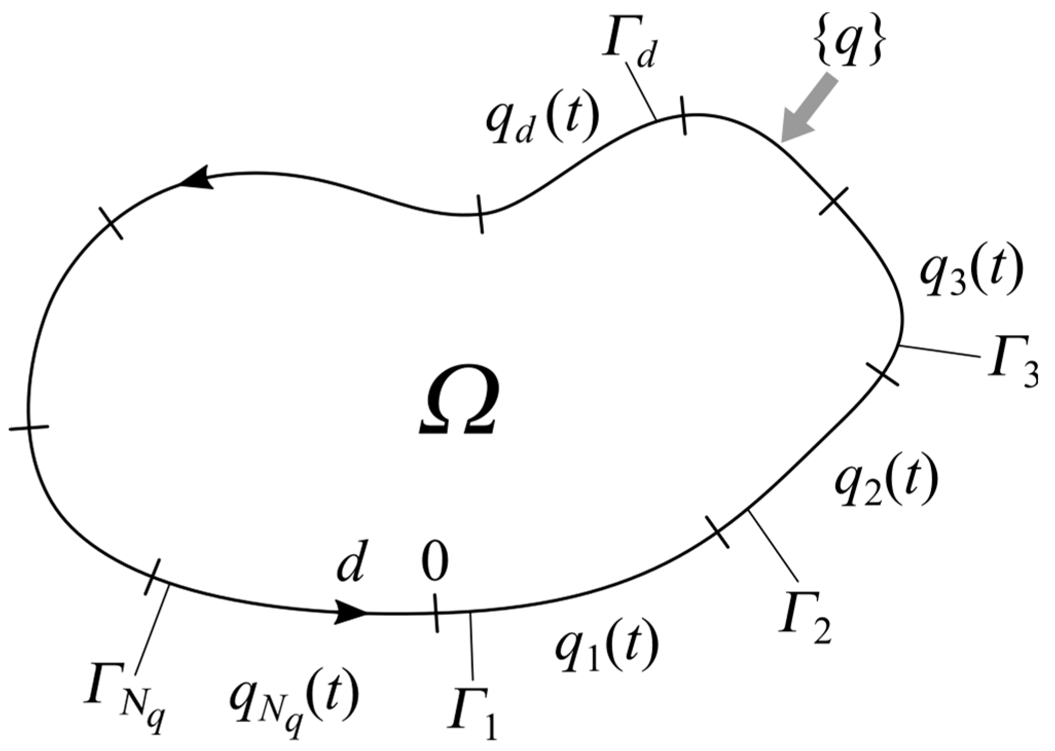
The following system of equations can solve transient heat conduction in the element, which is shown in Figure 1 [21]:

$$c\left(T\right)\rho \left(T\right)\frac{\partial T\left(x,y,z,t\right)}{\partial t}=\frac{\partial }{\partial x}\left[k\left(T\right)\frac{\partial T\left(x,y,z,t\right)}{\partial x}\right]+\frac{\partial }{\partial y}\left[k\left(T\right)\frac{\partial T\left(x,y,z,t\right)}{\partial y}\right] +\frac{\partial }{\partial z}\left[k\left(T\right)\frac{\partial T\left(x,y,z,t\right)}{\partial z}\right]$$

(1a)

$$T\left(x,y,z,t\right)=T_0\left(x,y,z\right) t=0$$

(1b)

$${-k\left(T\right)\frac{\partial T\left(x,y,z,t\right)}{\partial n}|}_{{\Gamma }_d}=q_d d=1, 2,\dots ,N_q, t>0$$

(1c)

Material properties are known functions of temperature (k—thermal conductivity, c—specific heat, ρ—density). The initial temperature distribution at time 0 s is T₀(x, y, z), and q_d(t) are heat fluxes on surfaces Γ_d.

If the CVM [22] is applied by dividing the domain into N_E control volumes, the set of Equation (1a) may be written in the matrix form

$$\left\{\dot{T}\right\}=\left[B\right]\left\{T\right\}+\left[C\right]\left\{q\right\}$$

(2)

with the initial condition

$$\left\{T\left(t_0\right)\right\}={\left\{\begin{array}{c}{T}_1\left(t_0\right)\\ T_2\left(t_0\right)\\ .\\ .\\ T_{N_E}\left(t_0\right)\end{array}\right\}}_{N_E}$$

(3)

where {T} is the N_E component column vector, which represents temperature changes in N_E nodes, time variable t varies between t₀ and t_N+1, [B] is the N_E × N_E component matrix, [C] is the matrix of N_E × N_q dimensions, and $\left\{q\right\}={\left\{q_1,q_2,\dots q_{N_q}\right\}}^T$ is the N_q—component column vector, which represents boundary heat flux changes. The spatial division and the choice of the time step affect the accuracy of the direct solution. The denser the discretization, the more accurate the solution will be. However, there is a point beyond which further compaction has no effect on the quality of obtained results. The matrix [B] in Equation (2) can be temperature-dependent. However, in the proposed method, it is determined only for selected temperatures for each prediction submodel that will be presented in Section 3.

The solution of Equation (2) in the form of a linear differential equation has the following matrix form [23]:

$$\left\{T\left(t\right)\right\}=e^{\left(t-t_0\right)\left[B\right]}\left\{T\left(t_0\right)\right\}+e^{t[B]}{\displaystyle {\int }_{t_0}^t{e}^{-s[B]}[C]\left\{q\left(s\right)\right\}}ds$$

(4)

Replacing t with t₀ + Δt in (4) gives:

$$\left\{T\left(t_0+\Delta t\right)\right\}=e^{\Delta t\left[B\right]}\left\{T\left(t_0\right)\right\}+e^{\left(t_0+\Delta t\right)[B]}{\displaystyle {\int }_{t_0}^{t_0+\Delta t}{e}^{-s[B]}[C]\left\{q\left(s\right)\right\}}ds$$

(5)

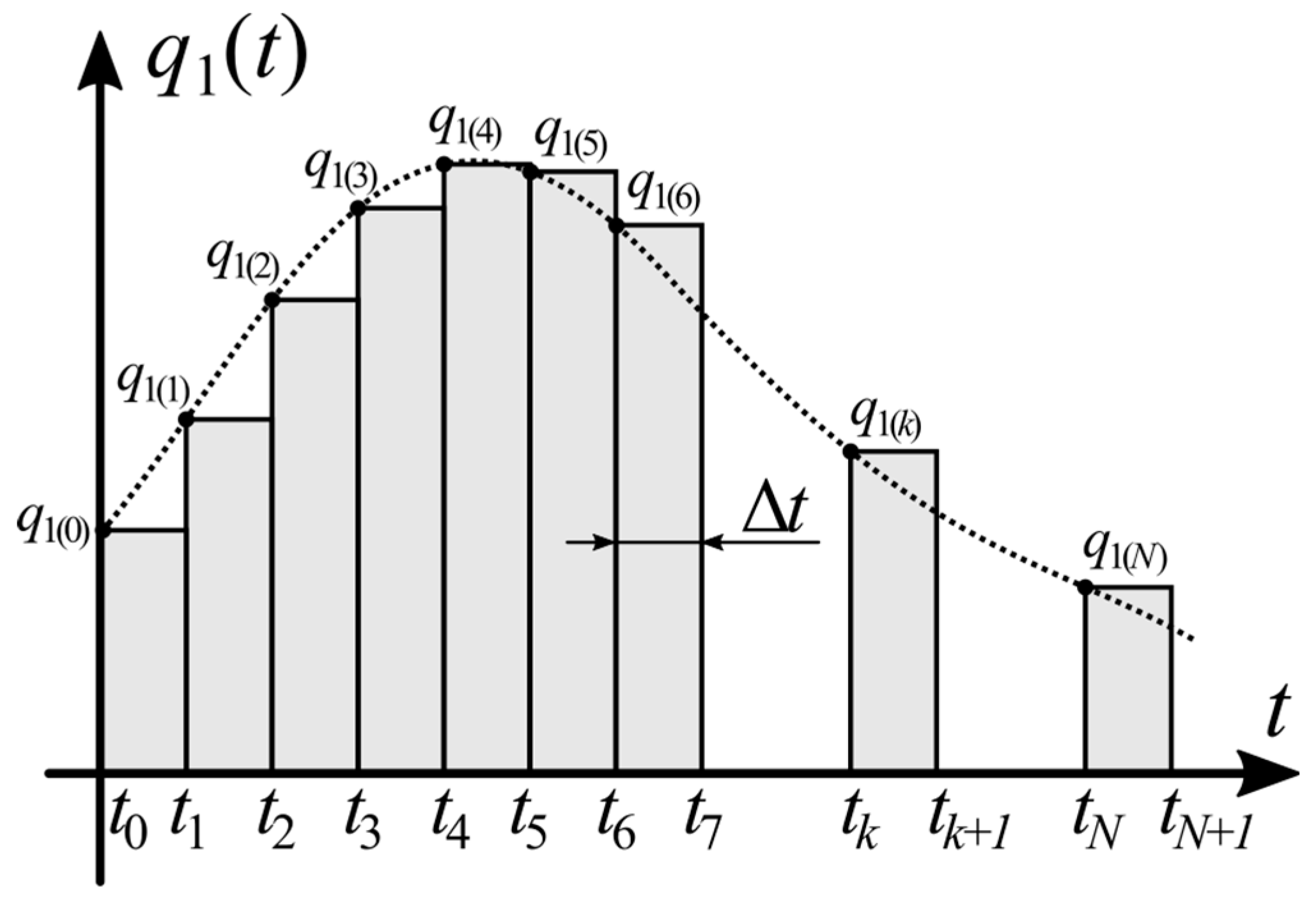
If heat fluxes q_d(t) on the boundary surfaces Γ_d are estimated by a staircase function versus time (cf. Figure 2),

$$\left\{\begin{array}{c}{q}_1(t)=q_1{}_{(k)}\\ \dots \\ q_d(t)=q_d{}_{(k)}\\ \dots \\ q_{N_q}(t)=q_{N_q}{}_{(k)}\end{array}\right\} k\Delta t<t<\left(k+1\right)\Delta t, k\in \langle 0,\dots ,N\rangle$$

(6)

Equation (5) can also be formulated as:

$$\left\{T\left(t_0+\Delta t\right)\right\}=\left[G\right]\left\{T\left(t_0\right)\right\}+\left[H\right]\left\{q_{\left(0\right)}\right\},$$

(7)

where

$$\left[G\right]=e^{\left[B\right]\Delta t,}$$

(8)

$$\left[H\right]={\displaystyle {\int }_{t_0}^{t_0+\Delta t}{e}^{\left(t_0+\Delta t-s\right)\left[B\right]}\left[C\right]ds}=-{\displaystyle {\int }_{\Delta t}^0{e}^{\tau \left[B\right]}\left[C\right]d\tau }={\displaystyle {\int }_0^{\Delta t}{e}^{\tau \left[B\right]}d\tau \left[C\right],}$$

(9)

where $\tau =t_0+\Delta t-s$.

Converting $e^{\Delta t\left[B\right]}$ into the McLaurin series-like function e^x, [G] has the form

$$\left[G\right]=\left[I\right]+\Delta t\left[B\right]+\frac{{\left(\Delta t\left[B\right]\right)}^2}{2!}+\frac{{\left(\Delta t\left[B\right]\right)}^3}{3!}+\frac{{\left(\Delta t\left[B\right]\right)}^4}{4!}\dots$$

(10)

Substituting $e^{\Delta t\left[B\right]}$ into Equation (9) and integrating gives

$$\left[H\right]=[\left[I\right]+\frac{\Delta t\left[B\right]}{2!}+\frac{{\left(\Delta t\left[B\right]\right)}^2}{3!}+\frac{{\left(\Delta t\left[B\right]\right)}^3}{4!}+\frac{{\left(\Delta t\left[B\right]\right)}^4}{5!}\dots ]\left[C\right]\Delta t$$

(11)

Using Equation (7), the temperature distribution in time t₁ can be formulated as:

$$\left\{T\left(t_1\right)\right\}=\left[G\right]\left\{T\left(t_0\right)\right\}+\left[H\right]\left\{q_{\left(0\right)}\right\}$$

(12)

Similarly, for time point t_2,

$$\left\{T\left(t_2\right)\right\}=\left[G\right]\left\{T\left(t_1\right)\right\}+\left[H\right]\left\{q_{\left(1\right)}\right\}$$

(13)

Substituting Equation (12) into (13) gives

$$\left\{T_{\left(2\right)}\right\}=\left[G\right]\left[\left[G\right]\left\{T_{\left(0\right)}\right\}+\left[H\right]\left\{q_{\left(0\right)}\right\}\right]+\left[H\right]\left\{q_{\left(1\right)}\right\},$$

(14)

which, after transformation, is

$$\left\{T_{\left(2\right)}\right\}={\left[G\right]}^2\left\{T_{\left(0\right)}\right\}+\left[G\right]\left[H\right]\left\{q_{\left(0\right)}\right\}+\left[H\right]\left\{q_{\left(1\right)}\right\},$$

(15)

and for point k (cf. Figure 2) is

$$\left\{T_{\left(k\right)}\right\}={\left[G\right]}^k\left\{T_{\left(0\right)}\right\}+{\displaystyle \sum _{j=0}^{k-1}{\left[G\right]}^{k-1-j}\left[H\right]\left\{q_{\left(j\right)}\right\}}$$

(16)

Equation (16) may be applied to obtain the temperature field in space for time t_k when all boundary heat fluxes $\left\{q_{\left(j\right)}\right\}={\left\{q_1{}_{\left(j\right)},q_2{}_{\left(j\right)},\dots q_{N_q}{}_{\left(j\right)}\right\}}^T$ for time j = 0 …, k − 1 are known. It is also a direct solution, like the CVM.

3. Formulation of the Method

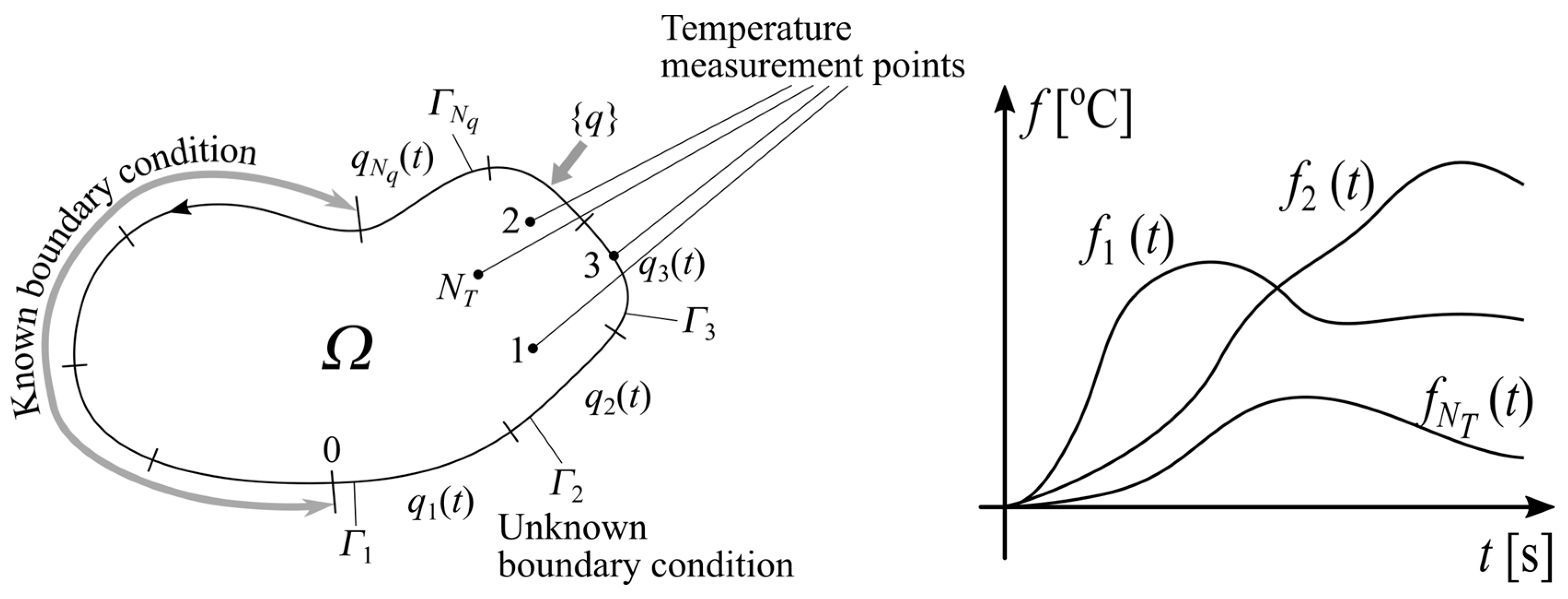
If boundary heat fluxes {q} are unknown in fragments of the domain border, the task becomes ill posed, and supplementary temperature measurements are necessary (Figure 3). They can be determined using the measured temperature histories in points 1 to N_T. In order to simplify the description, it was assumed that the number of unknown heat fluxes N_q and measuring points N_T are equal to 2. Temperature is measured in points 1 and 2 at instant k + 1, k + 2, …, k + N_F, which constitutes the corresponding inverse heat transfer problem. Here, N_F is the number of future time steps, and q_1(k) and q_2(k) are identified values of q₁(t) and q₂(t) for t = kΔt [24]. The following denotations are adopted: the subscript in parentheses means the temporal moment; the subscript without parentheses denotes the spatial point or the submodel number; and superscripts are reserved for exponentiation.

The system of Equations (1a) or (16) is nonlinear because thermal conductivity, specific heat, and density can be temperature functions. To determine matrix [B] in Equation (2) and matrices in subsequent equations, the temperature distribution should be known. Since the temperature distribution is sought, some starting temperature distribution can be assumed and the problem can be solved iteratively. Unfortunately, the computation time will then be extended and the inverse algorithm cannot be used in online mode. Therefore, a linearization of the problem is proposed. If several temperatures are selected within the range of the maximum temperature change, then one non-linear problem can be broken down into several linear problems. 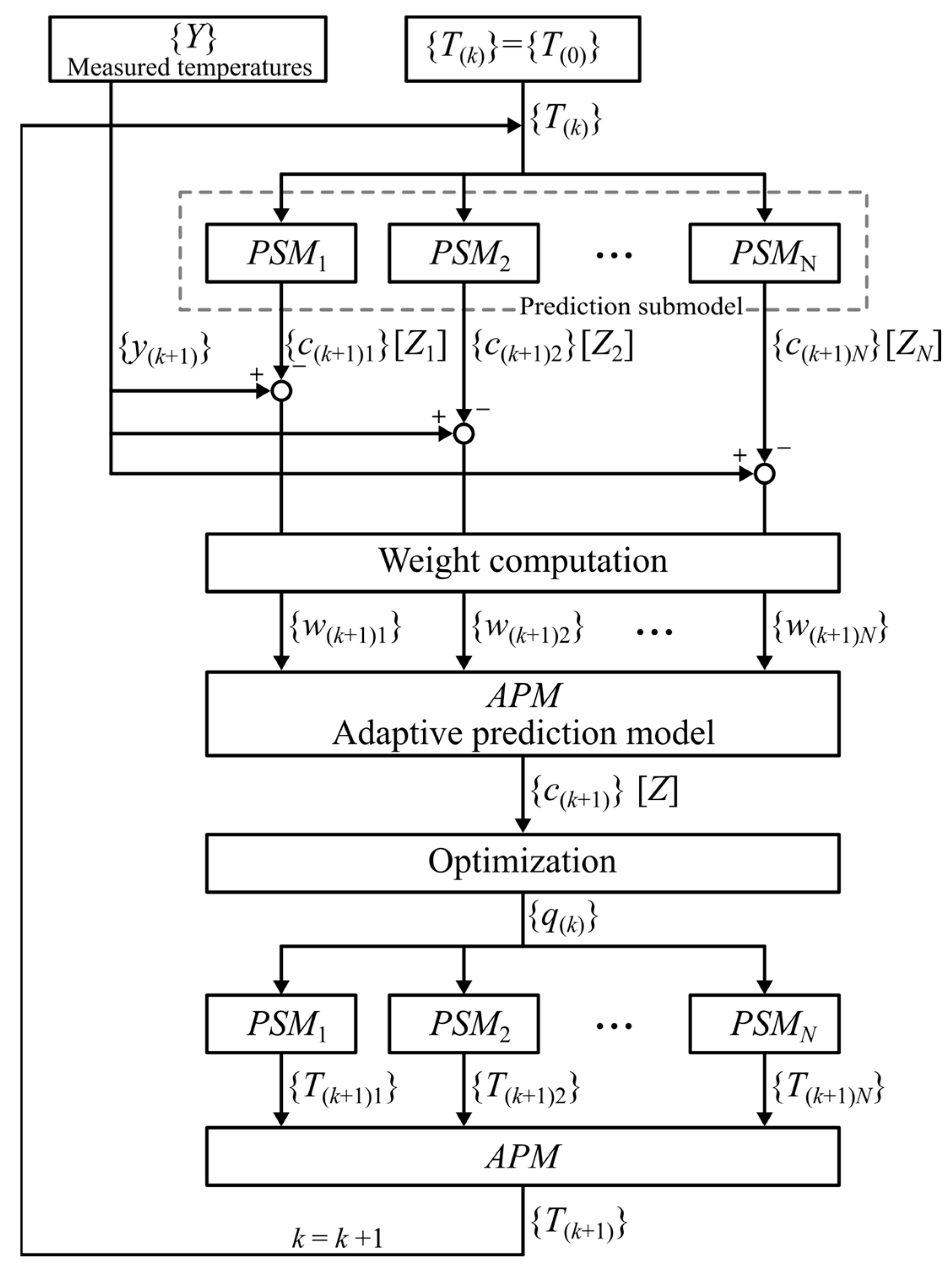In each of the linear problems, the matrix [B] and the following matrices can already be determined because the temperatures have been selected to determine them. The nonlinear problem is broken down into a number of linear heat transfer subspaces, which are described by submodels PSM_s (s = 1, 2, …, N) [20] (cf. Figure 4). The purpose of the PSMs model is to calculate the temperature history in places where this temperature is measured. For this purpose, the previously described equations are needed. The closer the temperature history calculated by a given submodel is to the measured temperature history, the better the given submodel fits the solution of non-linear problem. Finally, the results obtained from the submodels are combined into the final solution, the process of which is called the adaptation. Next, according to the matching degree between the temperatures measured {y_(k)} and calculated by submodels {c_(k)s} (s = 1, 2, …, N), they are weighted and combined to create the full adaptive prediction model (APM) for the solution of the nonlinear IHCP. Finally, boundary heat fluxes {q_(k)} are calculated. They are applied to determine the temperature distribution {T_(k+1)}, once again using the prediction submodels and the full adaptive prediction model.

In Figure 4, {Y} is the column vector due to the temperature variations in measuring points m = 1 and m = 2 from the beginning to the end of the analysed process. The 2*N_F dimensional column vector {y_(k+1)} contains the measured temperature histories in TC₁ and TC₂ at instant k + 1, k + 2, …, k + N_F.

The temperature values in the same spatial points and at the same time instants as in vector {y_(k+1)} can be calculated using Equation (16).

$$\left\{\begin{array}{c}{T}_{m=1\left(k+1\right)}\\ T_{m=1\left(k+2\right)}\\ ⋮\\ T_{m=1\left(k+N_F\right)}\\ T_{m=2\left(k+1\right)}\\ T_{m=2\left(k+2\right)}\\ ⋮\\ T_{m=2\left(k+N_F\right)}\end{array}\right\}=\left\{\begin{array}{c}\left\{v_{m=1}\right\}\left[G\right]\left\{T_{\left(k\right)}\right\}\\ \left\{v_{m=1}\right\}{\left[G\right]}^2\left\{T_{\left(k\right)}\right\}\\ ⋮\\ \left\{v_{m=1}\right\}{\left[G\right]}^{N_F-1}\left\{T_{\left(k\right)}\right\}\\ \left\{v_{m=2}\right\}\left[G\right]\left\{T_{\left(k\right)}\right\}\\ \left\{v_{m=2}\right\}{\left[G\right]}^2\left\{T_{\left(k\right)}\right\}\\ ⋮\\ \left\{v_{m=2}\right\}{\left[G\right]}^{N_F-1}\left\{T_{\left(k\right)}\right\}\end{array}\right\}+\left\{\begin{array}{c}\left\{v_{m=1}\right\}\left[H\right]\left\{q_{\left(k\right)}\right\}\\ \left\{v_{m=1}\right\}\left[G\right]\left[H\right]\left\{q_{\left(k\right)}\right\}+\left\{v_{m=1}\right\}\left[H\right]\left\{q_{\left(k+1\right)}\right\}\\ ⋮\\ \left\{v_{m=1}\right\}{\displaystyle \sum _{j=0}^{N_F-1}\left({\left[G\right]}^{N_F-1-j}\left[H\right]\left\{q_{\left(k+j\right)}\right\}\right)}\\ \left\{v_{m=2}\right\}\left[H\right]\left\{q_{\left(k\right)}\right\}\\ \left\{v_{m=2}\right\}\left[G\right]\left[H\right]\left\{q_{\left(k\right)}\right\}+\left\{v_{m=2}\right\}\left[H\right]\left\{q_{\left(k+1\right)}\right\}\\ ⋮\\ \left\{v_{m=2}\right\}{\displaystyle \sum _{j=0}^{N_F-1}\left({\left[G\right]}^{N_F-1-j}\left[H\right]\left\{q_{\left(k+j\right)}\right\}\right)}\end{array}\right\},$$

(17)

where $\left\{v_m\right\}$ is the N_E dimensional row vector

$$\left\{v_m\right\}=\left\{0,\dots ,a_m,\mathrm{...0}\right\} \mathrm{and} a_m=1$$

(18)

The term on the left and the first term on the right side of Equation (17) are noted as {T_(k+1)} and {c_(k+1)}, respectively. The second term on the right side of this equation may be transformed in the following way

$$\left[\begin{array}{cc}\left[Za\right]& \left[Zb\right]\\ \left[Zc\right]& \left[Zd\right]\end{array}\right]\left\{\begin{array}{c}{q}_{1\left(k\right)}\\ q_{1\left(k+1\right)}\\ ⋮\\ q_{1\left(k+N_F-1\right)}\\ q_{2\left(k\right)}\\ q_{2\left(k+1\right)}\\ ⋮\\ q_{2\left(k+N_F-1\right)}\end{array}\right\}=\left[Z\right]\left\{q_{\left(k\right)}\right\},$$

(19)

where

$$\left[Za\right]=\left[\begin{array}{cccc}\left\{v_{m=1}\right\}\left[H\right]{\left\{1 0\right\}}^T& 0& \cdots & 0\\ \left\{v_{m=1}\right\}\left[G\right]\left[H\right]{\left\{1 0\right\}}^T& \left\{v_{m=1}\right\}\left[H\right]{\left\{1 0\right\}}^T& \cdots & 0\\ ⋮& ⋮& ⋮& ⋮\\ \left\{v_{m=1}\right\}{\left[G\right]}^{N_F-1}\left[H\right]{\left\{1 0\right\}}^T& \left\{v_{m=1}\right\}{\left[G\right]}^{N_F-2}\left[H\right]{\left\{1 0\right\}}^T& \cdots & \left\{v_{m=1}\right\}\left[H\right]{\left\{1 0\right\}}^T\end{array}\right],$$

$$\left[Zb\right]=\left[\begin{array}{cccc}\left\{v_{m=1}\right\}\left[H\right]{\left\{0 1\right\}}^T& 0& \cdots & 0\\ \left\{v_{m=1}\right\}\left[G\right]\left[H\right]{\left\{0 1\right\}}^T& \left\{v_{m=1}\right\}\left[H\right]{\left\{0 1\right\}}^T& \cdots & 0\\ ⋮& ⋮& ⋮& ⋮\\ \left\{v_{m=1}\right\}{\left[G\right]}^{N_F-1}\left[H\right]{\left\{0 1\right\}}^T& \left\{v_{m=1}\right\}{\left[G\right]}^{N_F-2}\left[H\right]{\left\{0 1\right\}}^T& \cdots & \left\{v_{m=1}\right\}\left[H\right]{\left\{0 1\right\}}^T\end{array}\right],$$

$$\left[Zc\right]=\left[\begin{array}{cccc}\left\{v_{m=2}\right\}\left[H\right]{\left\{1 0\right\}}^T& 0& \cdots & 0\\ \left\{v_{m=2}\right\}\left[G\right]\left[H\right]{\left\{1 0\right\}}^T& \left\{v_{m=2}\right\}\left[H\right]{\left\{1 0\right\}}^T& \cdots & 0\\ ⋮& ⋮& ⋮& ⋮\\ \left\{v_{m=2}\right\}{\left[G\right]}^{N_F-1}\left[H\right]{\left\{1 0\right\}}^T& \left\{v_{m=2}\right\}{\left[G\right]}^{N_F-2}\left[H\right]{\left\{1 0\right\}}^T& \cdots & \left\{v_{m=2}\right\}\left[H\right]{\left\{1 0\right\}}^T\end{array}\right],$$

$$\left[Zd\right]=\left[\begin{array}{cccc}\left\{v_{m=2}\right\}\left[H\right]{\left\{0 1\right\}}^T& 0& \cdots & 0\\ \left\{v_{m=2}\right\}\left[G\right]\left[H\right]{\left\{0 1\right\}}^T& \left\{v_{m=2}\right\}\left[H\right]{\left\{0 1\right\}}^T& \cdots & 0\\ ⋮& ⋮& ⋮& ⋮\\ \left\{v_{m=2}\right\}{\left[G\right]}^{N_F-1}\left[H\right]{\left\{0 1\right\}}^T& \left\{v_{m=2}\right\}{\left[G\right]}^{N_F-2}\left[H\right]{\left\{0 1\right\}}^T& \cdots & \left\{v_{m=2}\right\}\left[H\right]{\left\{0 1\right\}}^T\end{array}\right]$$

The material properties depending on temperature are components of matrices [G] and [H]. The problem is easier to solve if the matrices are determined at a certain temperature. For this reason, submodels PSM_s (s = 1, 2, …, N) are built.

Temperatures {c_(k+1)s} predicted by submodels PSM_s can be compared to the measured values {y_(k+1)}, as presented in Figure 3. The bigger the deviation $\Vert \left\{c_{(k+1)s}\right\}-\left\{y_{(k+1)}\right\}\Vert$, the worse the adjustment of the prediction submodel PSM_s to the full model. The s = N normalized 2*N_F dimensional vectors {w_(k+1)s} are adopted:

$$w_{m\left(k+i\right)s}=\frac{\exp \left(-\left|y_{m\left(k+i\right)}-c_{m\left(k+i\right)s}\right|/\max \left|y_{m\left(k+i\right)}-c_{m\left(k+i\right)s}\right|\right)}{{\displaystyle \sum _{s=1}^N\exp \left(-\left|y_{m\left(k+i\right)}-c_{m\left(k+i\right)s}\right|/\max \left|y_{m\left(k+i\right)}-c_{m\left(k+i\right)s}\right|\right)}} i=1,\dots ,N_F-1; m=1,2; s=1,\dots ,N,$$

(20)

where subscript m is the measuring point number.

By using the prediction submodel weights, the prediction submodels PSM_s are weighted and combined to calculate {c_(k+1)} and [Z] as follows:

$$c_{m\left(k+i\right)}={\displaystyle \sum _{s=1}^N{w}_{m(k+i)s}{c}_{m\left(k+i\right)s}} i=1,\dots ,N_F-1; m=1,2,$$

(21)

$$Z_{m\left(k+i\right); m\left(k+i\right)}={\displaystyle \sum _{s=1}^N{w}_{m(k+i)s}{Z}_{m\left(k+i\right)s; m\left(k+i\right)s}} i=1,\dots ,N_F-1; m=1,2$$

(22)

The inverse method should find the unknown boundary condition {q_(k)} to keep calculated temperatures {T_(k+1)} close to the experimentally measured temperatures {y_(k+1)}.

$$\left\{y_{(k+1)}\right\}\cong \left\{T_{(k+1)}\right\}$$

(23)

The LSM is applied to fulfil this condition:

$${\displaystyle \sum _{m=1}^2{\displaystyle \sum _{i=1}^{N_F}{\left(y_{m\left(k+i\right)}-T_{m\left(k+i\right)}\right)}^2}}=\min$$

(24)

This can be written with a regularization term using Equation (17):

$$S={\Vert \left\{c_{\left(k+1\right)}\right\}+\left[Z\right]\left\{q_{\left(k\right)}\right\}-\left\{y_{\left(k+1\right)}\right\}\Vert }^2+\alpha {\Vert \left\{q_{\left(k\right)}\right\}\Vert }^2=\min ,$$

(25)

where α is a regularization parameter. Tikhonov regularization [25] can improve the IHCP stability. The solution that fulfils Equation (25) is

$$\left\{q_{\left(k\right)}\right\}={\left({\left[Z\right]}^T\left[Z\right]+\left[R\right]\right)}^{-1}{\left[Z\right]}^T\left(\left\{y_{\left(k+1\right)}\right\}-\left\{c_{\left(k+1\right)}\right\}\right),$$

(26)

where

$$\left[R\right]=\left[\begin{array}{cccccc}{\alpha }_1& \cdots & 0& 0& \cdots & 0\\ ⋮& ⋮& ⋮& ⋮& ⋮& ⋮\\ 0& \cdots & {\alpha }_1& 0& \cdots & 0\\ 0& \cdots & 0& {\alpha }_2& \cdots & 0\\ ⋮& ⋮& ⋮& ⋮& ⋮& ⋮\\ 0& \cdots & 0& 0& \cdots & {\alpha }_2\end{array}\right]$$

(27)

Here, α₁ and α ₂, respectively, are the regularization parameters for heat fluxes q₁(t) and q₂(t). To determine temperature {T_(k+1)}, submodels PSM_s (s = 1, 2, …, N) are built, weighted, and combined once again. After temperature {T_(k+1)} is obtained, the next time point can be analysed until the end of the process t = N_tΔt.

4. Numerical Verification

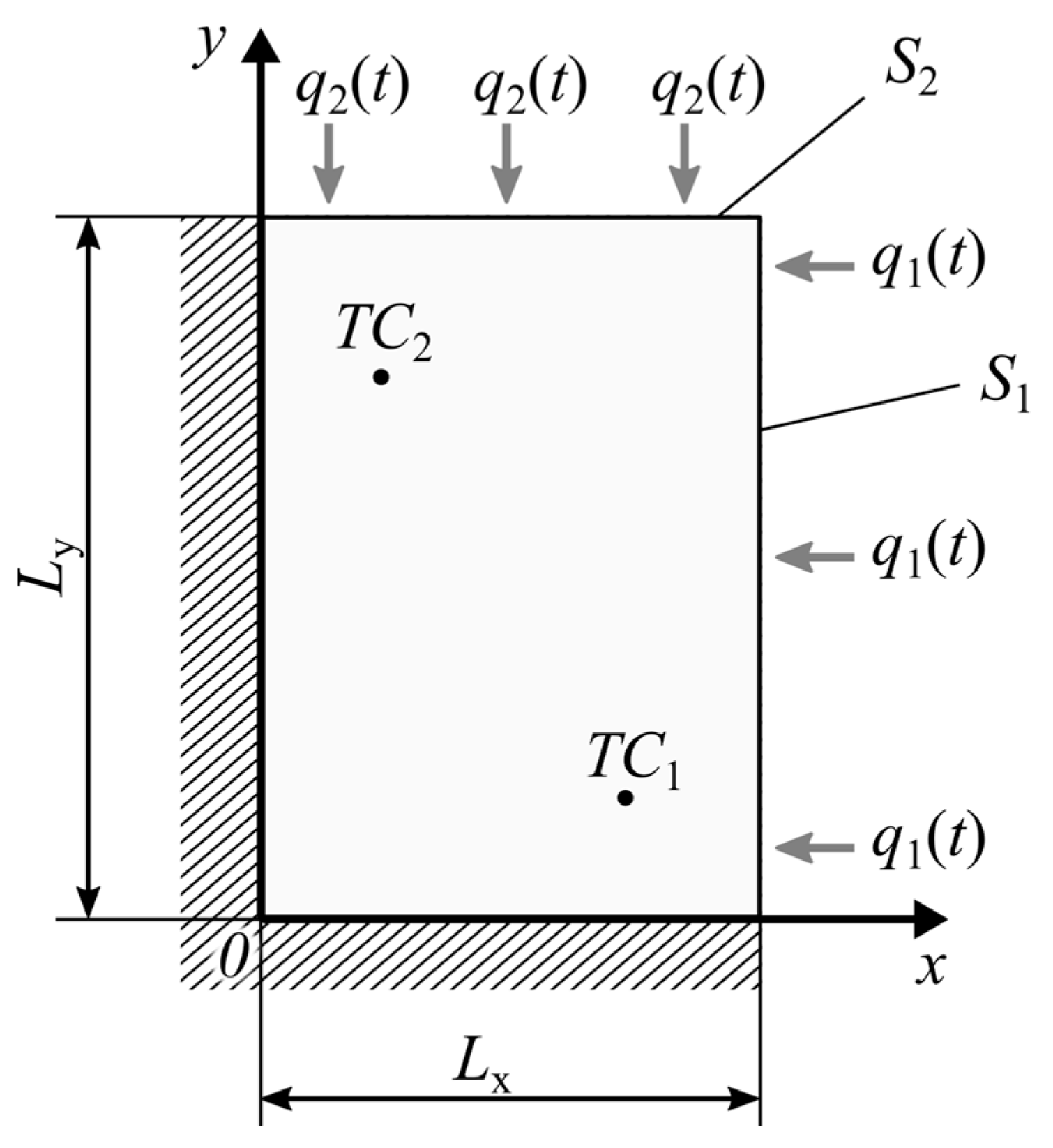
The above-developed algorithm is used for temperature estimation in the plate presented in Figure 5. It is made of a steel 17M0V84mod [26]. Its temperature-dependent properties are shown in

Table 1. Thermophysical properties of 17M0V84mod steel.

T [°C]	k [W/(m K)]	c [J/(kg K)]	ρ [kg/m3]
20	46.7	527.5	7800
100	49.8	580.4	7800
200	52.8	599.9	7800
300	50.5	489.3	7800

.

The following dimensions and initial and boundary conditions are used: L_x = 750 mm, L_y = 150 mm, T_(x,y,t=0) = 20 °C,

$$q_1\left(t\right)=1.8\times {10}^5\left(1-{\mathrm{e}}^{-0.1t}\right)+1.5\times {10}^5\sin \left(\frac{\pi t}{60}\right) [\raisebox{1ex}{$\mathrm{W}$}\!\left/ \!\raisebox{-1ex}{${\mathrm{m}}^2$}\right.],$$

(28a)

$$q_2\left(t\right)=\{\begin{array}{ll}0\left[\raisebox{1ex}{$\mathrm{W}$}\!\left/ \!\raisebox{-1ex}{${\mathrm{m}}^2$}\right.\right]& t<30 \mathrm{s}\\ 3\times {10}^5 \left[\raisebox{1ex}{$\mathrm{W}$}\!\left/ \!\raisebox{-1ex}{${\mathrm{m}}^2$}\right.\right]& 30 \mathrm{s}\le t\le 72 \mathrm{s}\\ 0 \left[\raisebox{1ex}{$\mathrm{W}$}\!\left/ \!\raisebox{-1ex}{${\mathrm{m}}^2$}\right.\right]& t>72 \mathrm{s}\end{array}$$

(28b)

Rapid time- and space-dependent changes in the heat flux take place in the power boiler furnace, for example. The curves are intended to test the method so that it can be used in practice in the future. The following number of spatial divisions, time step size, and number of future steps are adopted: l_x = 6, l_y = 8; Δt = 0.6 s; N_F = 5. Temperature measuring points are located in TC₁ (2L_x/3, L_y/2) and TC₂ (2L_x/3, 7L_y/8), respectively. Like in the direct solution, spatial division and the choice of the time step affect the accuracy of the inverse method. However, excessive compaction may not improve the quality of the solution, but rather reduce its stability. The solution stability also depends on the number of future time steps N_F. The method becomes unstable if it is insufficient. In contrast, when it is too big, there is a rise in solution errors. The choice of the time and space division can be similar to the selection made in the direct solution. The number of future steps can be selected using the iterative method. A gradual reduction in their number increases the method instability. The location of measuring points also has a great impact on the solution’s accuracy and stability. An increase in the distance of the measuring points from the edges with unknown boundary conditions deteriorates the solution stability and accuracy.

The root mean square error (RMSE) [27] and the average relative error of the identified temperature is proposed to estimate the accuracy of the method:

$$S_T=\sqrt{\frac{1}{N_E{N}_t}{\displaystyle {\sum }_{m=1}^{N_E}{\displaystyle {\sum }_{k=l}^{N_t}{\left(T_{m\left(k\right), exa}^{}-T_{m\left(k\right)}^{}\right)}^2}}} ,$$

(29)

$${\eta }_T=S_T \raisebox{1ex}{${}_{}^{}$}\!\left/ \!\raisebox{-1ex}{${}_{}^{}$}\right. \sqrt{\frac{1}{N_E{N}_t}{\displaystyle {\sum }_{m=1}^{N_E}{\displaystyle {\sum }_{k=l}^{N_t}{\left(T_{m\left(k\right), exa}^2\right),}^{}}}}$$

(30)

where N_t represents the whole number of time steps and $T_{\left(k\right)m, exa}^{}$ shows the exact value of T_m(t) at the kth instant.

Additionally, the average relative error of the estimated heat flux is introduced:

$${\eta }_{q_m}=\sqrt{\frac{1}{N_t}{\displaystyle {\sum }_{k=l}^{N_t}{\left(q_{m\left(k\right), exa}^{}-q_{m\left(k\right)}^{}\right)}^2}} \raisebox{1ex}{${}_{}^{}$}\!\left/ \!\raisebox{-1ex}{${}_{}^{}$}\right. \sqrt{\frac{1}{N_t}{\displaystyle {\sum }_{k=l}^{N_t}{\left(q_{m\left(k\right), exa}^{}\right)}^2}} \left(m=1, 2\right),$$

(31)

where $q_{m\left(k\right), exa}^{}$ means the exact value of q_m(t) at the kth moment.

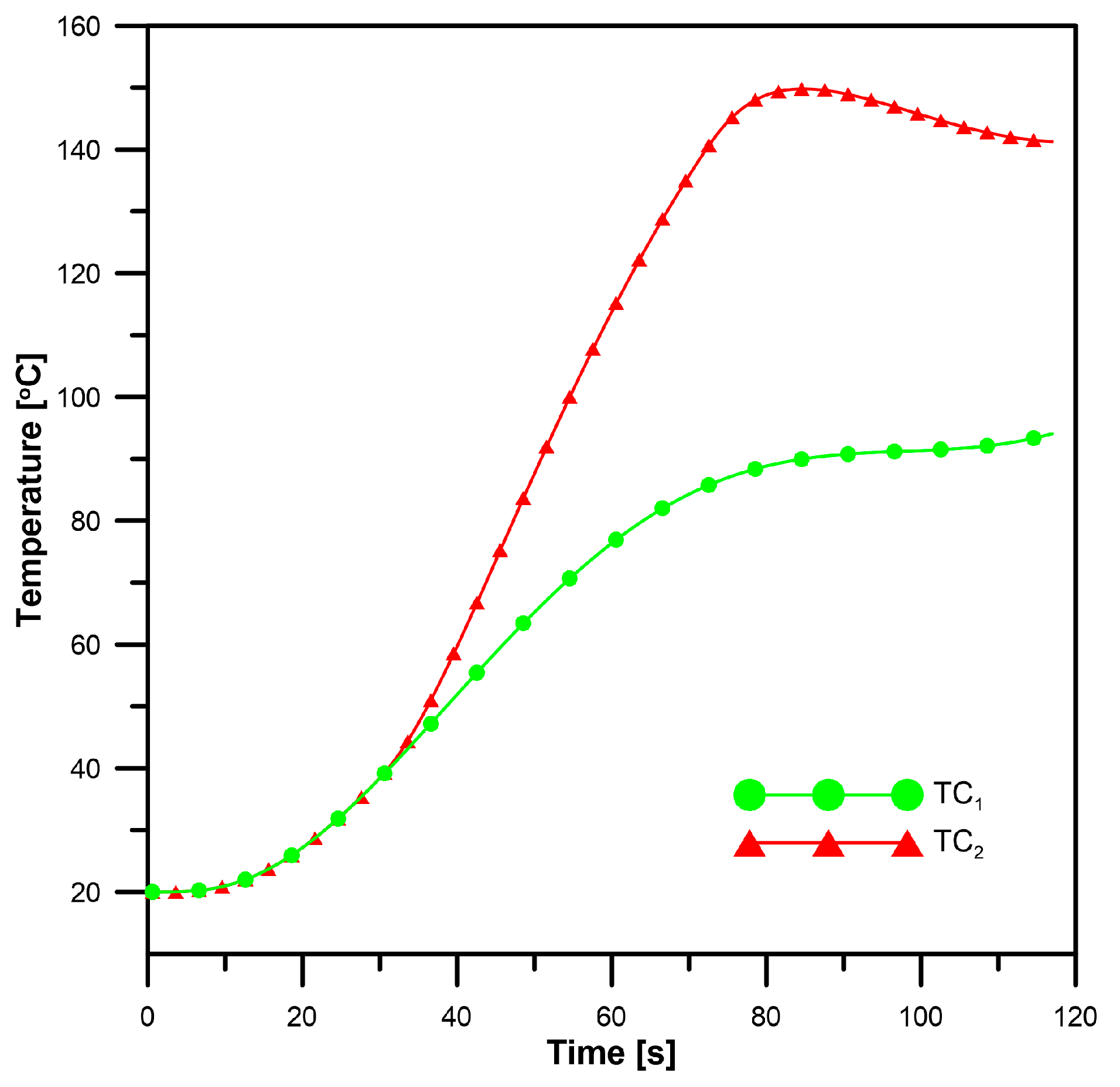
To solve the inverse boundary problem, temperature changes “measured” in points TC₁ and TC₂ are used. The curves are computed by a direct method using the FEM and the mesh densified twice (Figure 6). They may be applied as “undisturbed measuring” data ($Y_{m(k)}{}_{, exa}$) to verify the proposed method.

The number of submodels (N) depends on the material nonlinearities in the analysed temperature changes. Greater changes in material properties with temperature require more submodels. For the problem under consideration, the influence of N on accuracy is analysed as can be seen in

Table 2. Calculation time and obtained errors for the three methods with σ = 0.

Method	Calculation Time [s]	ST [°C]	ηT [%]	η [%] (q1)	η [%] (q2)
AMI (N = 2)	55	2.997	3.294	9.310	14.66
AMI (N = 4)	127	1.798	1.976	6.265	14.18
AMI (N = 5)	193	1.685	1.853	5.802	14.26
AMI (N = 6)	227	1.648	1.812	5.764	14.41
AMI (N = 8)	445	1.592	1.750	6.094	15.12
AMI (N = 10)	912	1.583	1.740	6.257	15.28
MMAI (N = 5)	56	-	-	8.837	18.29
LMA	6600	-	-	5.036	30.66

. The greater the N, the smaller the errors S_T and η_T are. Analysing errors ${\eta }_{q_1}$ and ${\eta }_{q_2}$, the best results are obtained for N = 5, and the corresponding set of prediction submodels is Ω = {PSM₁(20), PSM₂(90), PSM₃(160), PSM₄(230), PSM₄(300)}.

The golden section search method [28] is employed to find regularization parameters in Equation (27) to minimize the average relative error in Equation (30). The time to find the regularization coefficients is not taken into account in calculation times, which are presented in Table 2 and

Table 3. Calculation time and obtained errors for different σ.

σ	Method	Calculation Time [s]	ST [°C]	ηT [%]	η [%] (q1)	η [%] (q2)
0.001	AMI	216	1.686	1.853	5.802	14.26
	MMAI	89	-	-	8.891	18.32
0.03	AMI	219	1.774	1.905	10.32	20.50
	MMAI	57	-	-	12.04	25.77
0.05	AMI	206	1.847	2.030	16.72	26.52
	MMAI	88	-	-	19.29	34.08

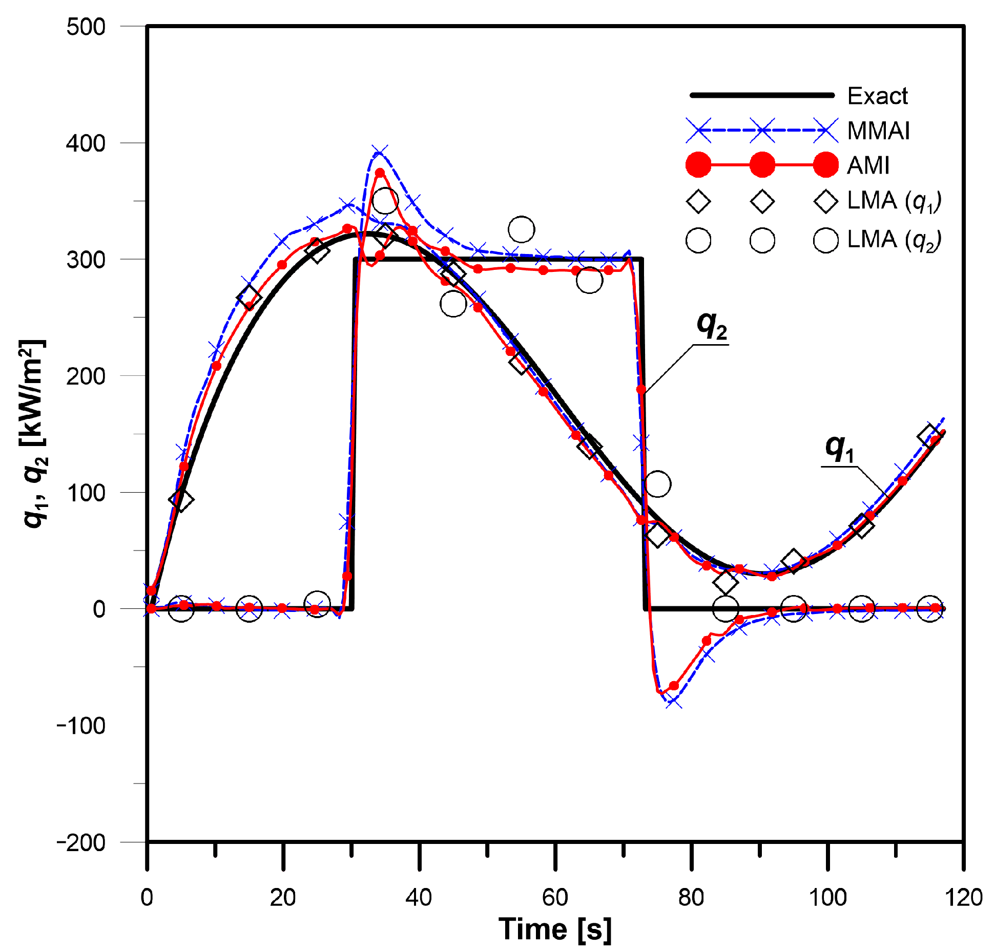
. The following values are applied for the proposed inverse method: α₁= 2.5 × 10⁻¹³, α₂ = 0.5 × 10⁻¹³. The heat fluxes identified by the AMI and MMAI methods for the number of submodels (N = 5) are presented in Figure 7. The exact fluxes are taken from Equation (28a,b). The obtained calculation time and errors are written in Table 2. In both methods, the code is written in the Matlab program. An Intel i7-4700HQ 2.4 GHz processor with 8 GB of RAM is used. The computation of the AMI method takes more time, but the identified heat fluxes are closer to the exact values. The MMAI method is faster because it calculates the temperature only in measurement points TC₁ and TC₂.

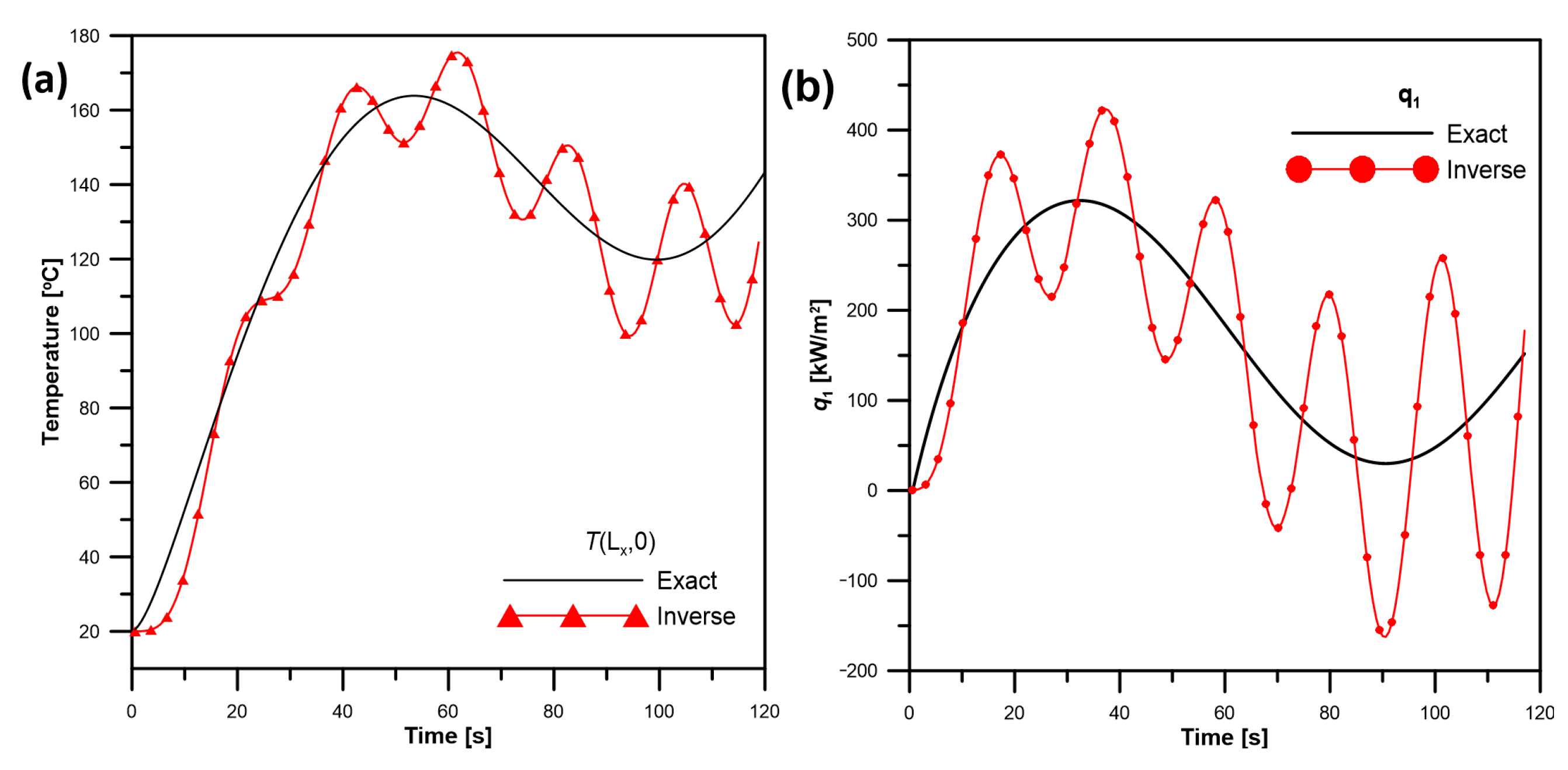
The decrease in the proposed method stability can be observed as oscillations of the determined quantities. Reducing the number of future steps N_F from five to two may reveal the oscillations, which are shown in Figure 8. This is the reason of the identification error increase to the values: S_T = 4.91 °C, η_T = 5.40%, η_q1 = 38.19%, and η_q2 = 55.64%. If the regularization coefficients are additionally lowered, the solution becomes completely unstable, giving the following errors: S_T = 5.E99 °C, η_T = 6.E99%, η_q1 = 5.7E90%, and η_q2 = 8.3E105%.

Additionally, the method based on the LMA algorithm is tested [9,10]. This procedure allows for the use of ANSYS Multiphysics software [29]. Temperature measurement points have to be moved to TC₁ (11L_x/12, L_y/2) and TC₂ (2L_x/3, 15L_y/16) to obtain a stable solution. The appropriate temperature changes are generated by the direct method. The number of future steps must also be increased to N_F = 10. Despite all these actions, the errors and computation time are much higher than in the AMI and MMAI methods.

The errors shown in Table 2 are created by the inverse problem’s ill-conditioning. Despite the considerable distance of the thermocouples from the unknown boundary conditions, the errors are not high. The AMI method for N = 5 allows the best identification of the unknown boundary conditions, and the mean error of the calculated temperature distribution does not exceed 1.7 °C and 1.9%.

To approach real conditions, “noisy measuring” data $Y_{(k)m}$ are calculated by summing normal random errors and “undisturbed measuring” data.

$$Y_{(k)m}=Y_{(k)m,}{}_{exa}+\omega \sigma$$

(32)

where ω is the random value of normal distribution with zero mean over the range [−2.576, 2.576], and σ is the measuring error standard deviation.

The number of submodels is (N = 5). For the disturbed data, the computing time by the AMI method also takes more time than by the MMAI method, as can be seen in Table 3. As the measuring error standard deviation σ increases, the errors in the identified temperature and heat fluxes (S_T, η_T and η_q) become greater. 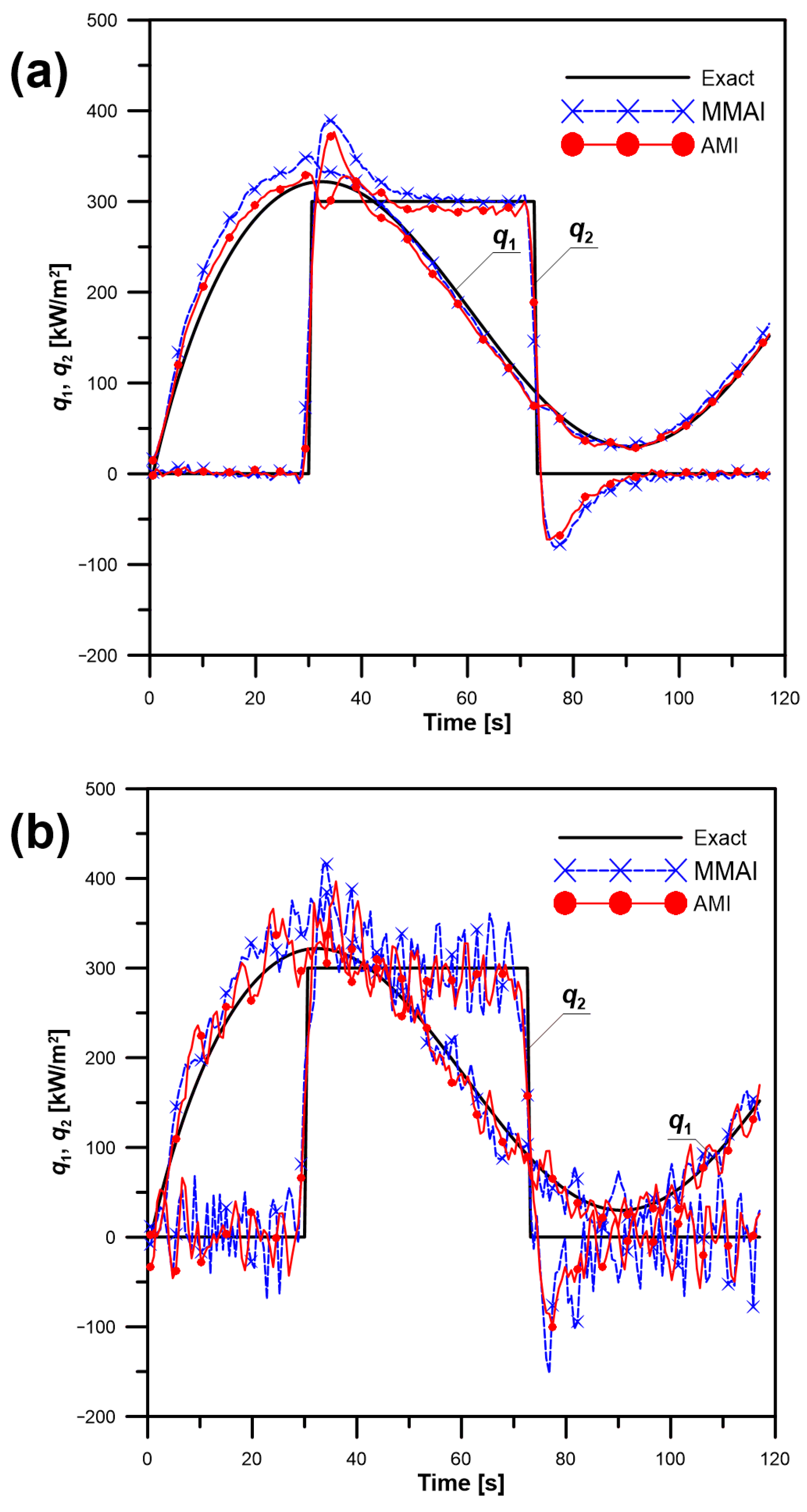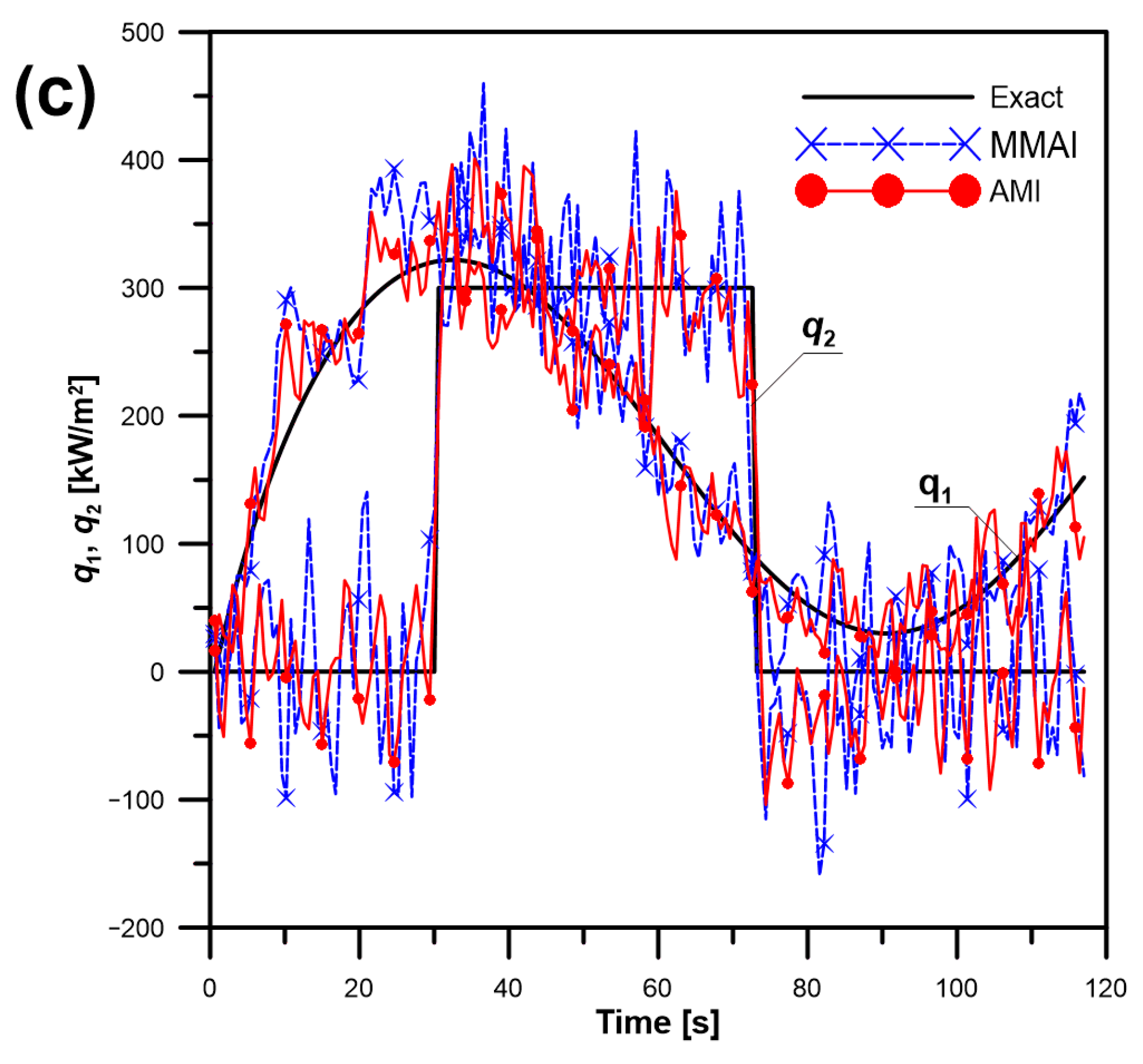For stronger disturbance, the regularization coefficients were different for every noise and were raised to the values of α₁= 9.8 × 10⁻¹³ and α₂ = 1.96 × 10⁻¹³. 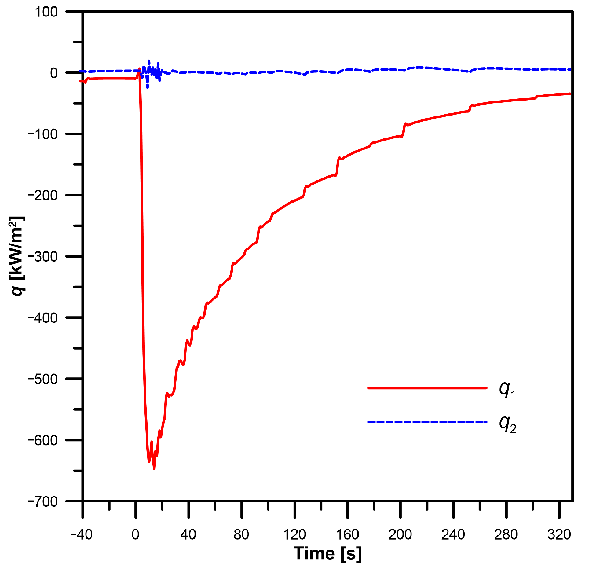The heat fluxes identified by the AMI method are close to the exact values, as can be seen in Figure 9. 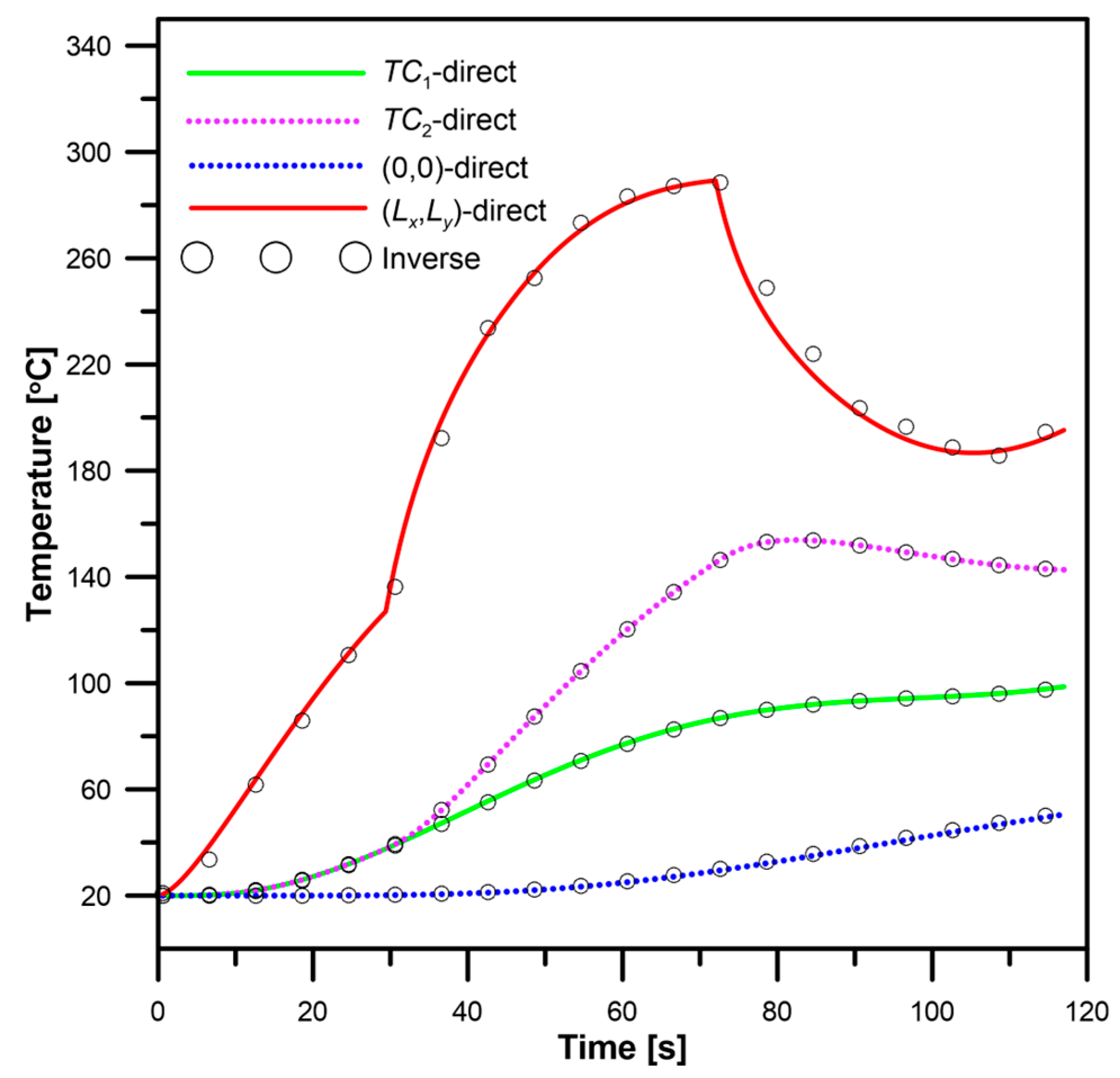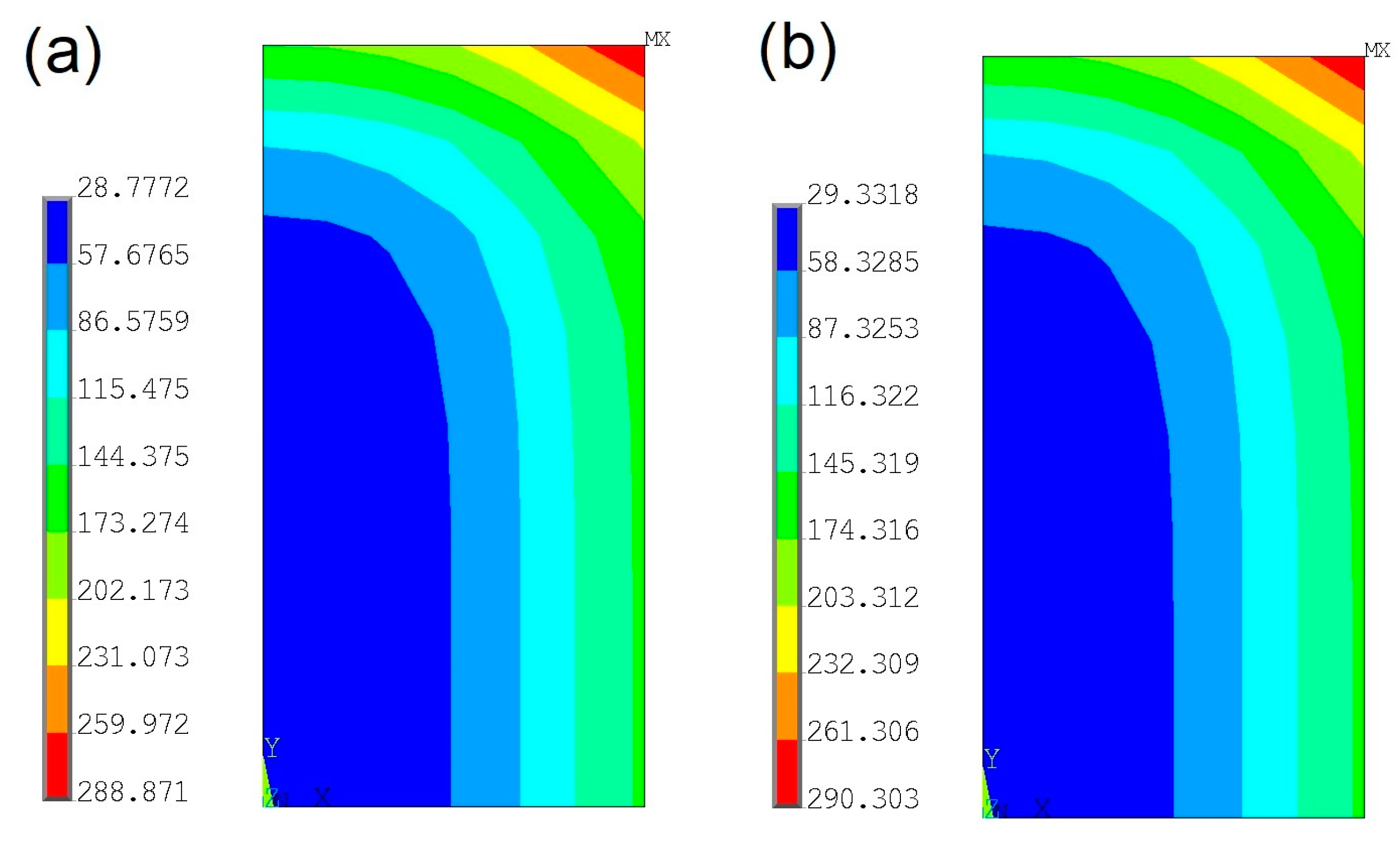Despite the introduced measuring errors and very difficult conditions of the test (flux q₂ suddenly changes from zero to 300 kW/m²), the mean error of the calculated temperature distribution does not exceed 1.9 °C and the relative error is about 2%. Comparisons of temperature calculated by a direct method and by the AMI method are presented in Figure 10 and Figure 11.

Both methods enabled accurate identification of unknown boundary conditions from the beginning of the heating process when a uniform temperature distribution appeared.

The additional advantage of the AMI method is that it can be used when the element’s initial temperature distribution is non-uniform. During long-term online identification, the system may crash and the algorithm must be restarted. The method, which is based on the superposition method, should analyse the process from the moment that the temperature distribution is uniform. This means that in the event of a system failure, the analysis must be repeated from the very beginning of the process. The AMI method is free from this disadvantage—it can be launched at any time during the process.

To demonstrate this capacity of the AMI method, the previously analysed heating process is identified starting halfway through the heating process. If the algorithm determining temperature is stopped after 51 s, the AMI method can start computations based on the determined temperature field at the previous time instant (50.4 s) and using the measured temperature histories in points TC₁ and TC₂. If the time is counted from the system restart, the measured temperature curves take the form given in Figure 12. The errors of the computed temperature and heat fluxes are S_T = 1.370 °C, η_T = 1.272%, η_q1 = 6.327%, and η_q2 = 17.96%. If the method that is based on the superposition algorithm is restarted after the interruption, and considering the last measurements before the system crashed as the starting condition, it becomes completely unstable.

The heat fluxes identified by the AMI method are given in Figure 13. Although the initial heat fluxes after the restart are not given, the AMI method enables their precise identification.

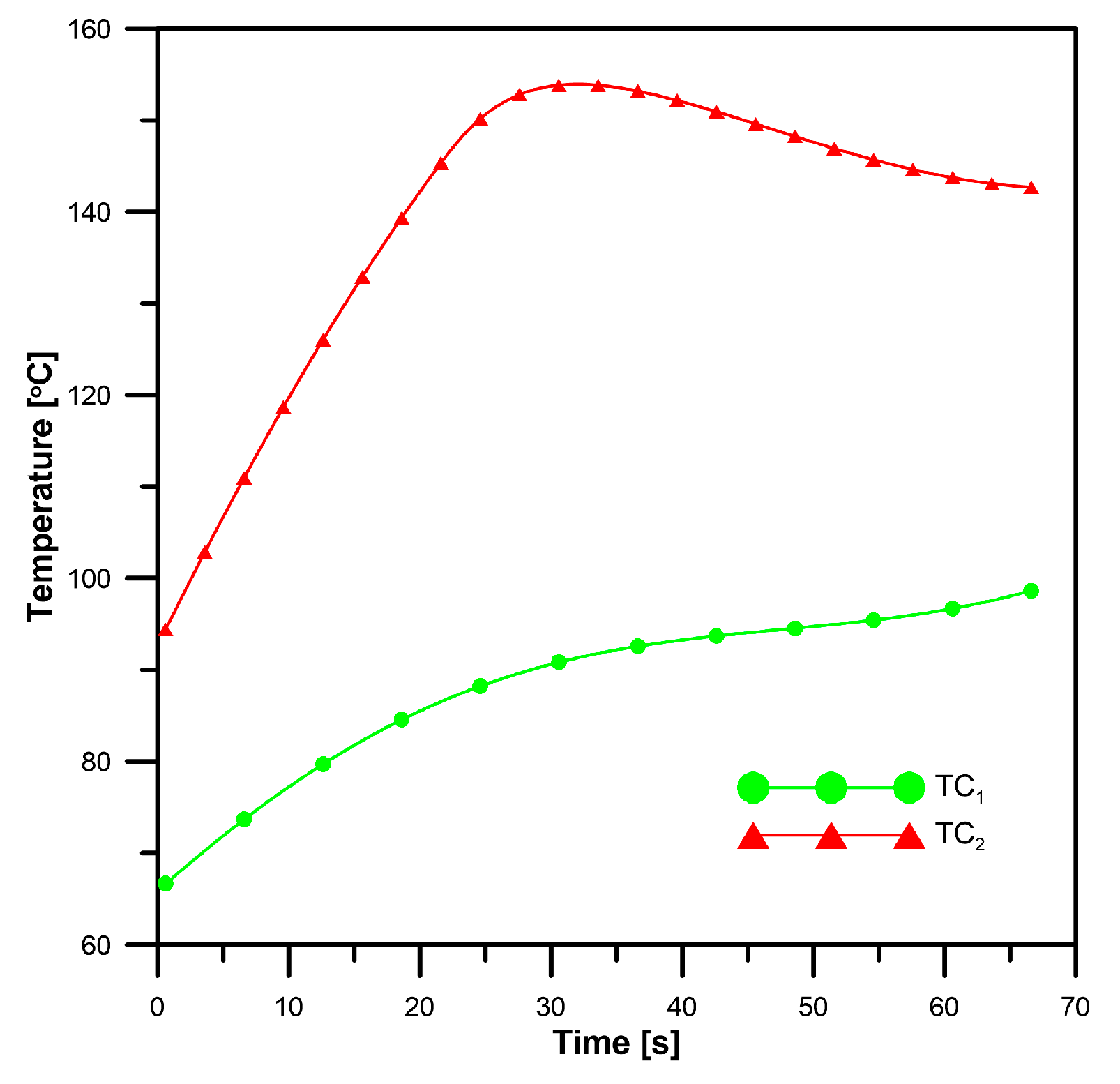
The proposed AMI method can also be used for bodies with irregular geometry. The control volume-FEM is used [30] instead of the CVM. The plate from previous analyses is deformed to the form shown in Figure 14. The same material properties and the same initial and boundary conditions as before are used to generate “measured” temperature histories in points TC₁ and TC₂, which are needed for the inverse boundary problem. The histories calculated using a direct solution based on the control volume-FEM are presented in Figure 15. Despite the irregular geometry resulting in irregular control volumes, the unknown heat fluxes identified by the AMI method are close to the exact values, which can be seen in Figure 16. The average errors in the estimated temperature and heat fluxes are S_T = 1.780 °C, η_T = 2.068%, η_q1 = 3.715%, and η_q2 = 18.36%. If the measuring points are shifted to the middle of the edges of S₁ and S₂, the errors will drop to η_q1 = 1.240% and η_q2 = 2.881%.

5. Experimental Verification

The experiment is carried out on a thick-walled cylinder, presented in Figure 17a. It is made of 17M0V84mod steel. Its temperature-dependent thermal properties are presented in Table 1 [26]. Six thermocouples for measuring wall temperature are located along the cylinder wall thickness (cf. Figure 17b). After completing the installation of the thermoelements, an electric resistance heating system is mounted on the cylinder outer surface, and insulation covers it. The thick-walled cylinder is heated to a temperature of 300 °C. Next, it is cooled by an injection of cold water, which flows through the spraying device inside the cylinder. The measured temperature histories in six points and the water temperature are shown in Figure 18.

The outer surface of the cylinder’s model is insulated, while an unknown thermal boundary condition appears on the inner one. The measured temperature history in point r₂ = 50 mm is used to solve the problem, which is defined in this way. For the problem under consideration, the influence of the number of submodels (N) on accuracy is analysed, as can be seen in

Table 4. Calculation time and errors obtained by the AMI method for different measurement points.

Measurement Point	N	Calculation Time [s]	ST [°C]	ηT [%]
T1 = T (r = 45 mm)	2	28	2.473	1.537
T2 = T (r = 50 mm)	1	10	3.185	2.016
T2 = T (r = 50 mm)	2	39	2.350	1.481
T2 = T (r = 50 mm)	3	79	2.309	1.451
T2 = T (r = 50 mm)	4	113	2.356	1.479
T2 = T (r = 50 mm)	5	171	2.394	1.503
T3 = T (r = 55 mm)	3	89	2.474	1.539
T4 = T (r = 60 mm)	3	63	2.798	1.747

. The best results are obtained for N = 3, and the corresponding set of prediction submodels is Ω = {PSM₁(30), PSM₂(165), PSM₃(300)}. The temperature histories identified by the AMI method for the number of submodels (N = 3) are compared to the measured temperature histories, as shown in Figure 18. The mean error of the calculated temperature distribution and relative error are S_T = 2.31 °C and η_T = 1.45%, respectively. If the inverse solution is based on temperature history in point r₁, r_3, or r_4, the errors are slightly larger, as presented in Table 4.

A further improvement in the solution accuracy can be obtained by adding the temperature history to the analysis, which is measured on the cylinder’s outer surface. In this way, the boundary condition on the outer surface can also be identified. The influence of the number of submodels (N) on accuracy is analysed, as is presented in

Table 5. Calculation time and errors obtained by the AMI method for two measurement points.

Measurement Point	N	Calculation Time [s]	ST [°C]	ηT [%]
T2 = T (r = 50 mm) and T6 = T (r = 80 mm)	1	52	1.995	1.253
T2 = T (r = 50 mm) and T6 = T (r = 80 mm)	2	94	1.902	1.196
T2 = T (r = 50 mm) and T6 = T (r = 80 mm)	3	226	1.916	1.204
T2 = T (r = 50 mm) and T6 = T (r = 80 mm)	4	373	1.922	1.208
T2 = T (r = 50 mm) and T6 = T (r = 80 mm)	5	622	1.925	1.209

. The best results are obtained for N = 2, and the corresponding set of prediction submodels is Ω = {PSM₁(20), PSM₂(300)}. The mean error of the calculated temperature distribution and relative error are S_T = 1.90 °C and η_T =1.20%, respectively. The identified heat fluxes are shown in Figure 19. A low heat flux q₂ on the outer surface indicates that the thermal insulation is good but not perfect in reality.

The uncertainties of the determined parameters were estimated using the error propagation rule of Gauss [31]. The following equation is used for the heat flux or temperature uncertainty calculation caused by temperature measurement errors:

$$2{\sigma }_{x_i}={\left[{\displaystyle \sum _{m=1}^{N_T}{\left(\frac{\partial x_i}{\partial f_m}2{\sigma }_{f_m}\right)}^2}\right]}^{0.5} i=1,2,3$$

(33)

The 95% uncertainty in the estimated parameters can be expressed in the form

$$x_i=x_i^{*}\pm 2{\sigma }_{x_i}$$

(34)

where $x_i^{*}$ represent the value of parameters obtained using the proposed inverse method (q₁, q₂, T). To show the influence of measurement errors on the determined heat fluxes or temperature, the 95% confidence intervals were calculated. The following uncertainties of measured temperatures are assumed: $2{\sigma }_{f_m}=\pm 0.258 K, m=1,\dots ,N_T$.

The uncertainties of the determined parameters were calculated for the assumed heat fluxes, which are shown in Figure 20. The calculation yielded the following results:

$$2{\sigma }_{q_1}=17647 \left[\mathrm{W}/{\mathrm{m}}^2\right], 2{\sigma }_{q_2}=2292 \left[\mathrm{W}/{\mathrm{m}}^2\right], 2{\sigma }_T=0.256 \left[\mathrm{K}\right]$$

Uncertainties for heat fluxes apply to the entire analysis period, and the calculated temperature uncertainty relates to the entire time–spatial temperature distribution.

6. Summary and Conclusions

An adaptive matrix inverse (AMI) method is presented to identify the temperature and unknown boundary heat flux distribution in a domain of a regular or irregular shape with temperature-dependent properties. The nonlinear IHCP is broken down into a number of linear submodels, and for each submodel, the temperature is obtained in measuring points. Next, based on the matching degree between the temperatures measured and calculated by each prediction submodel, the submodels are weighted and combined to create the full model for the solution of a nonlinear IHCP. Comparisons are also conducted with the existing MMAI procedure and the method based on the LMA algorithm, which are described in the literature.

The results of the presented numerical tests for undisturbed and disturbed “measuring” data indicate that the heat fluxes identified by the AMI method are the closest to the exact values. The MMAI method is faster because it calculates the temperature only in measurement points. The LMA method is the least accurate and it needs the longest time to perform the identification. A poorer accuracy and longer computation time are compensated for by a friendlier algorithm, which allows for the implementation of commercial calculation programs.

The presented method can be applied in an online mode due to the non-iterative nature of the computations. The measuring points can be located anywhere in the calculation domain to improve the solution quality. Unlike the inverse methods presented before, the proposed method can be launched at any time during the analysed process, and measuring points can be located anywhere in the calculation domain to improve the solution quality. The layout of measuring points is only limited by measurement possibilities, but it affects the solution accuracy. The proposed AMI method is well suited to online diagnostic systems.

The AMI method has been experimentally verified during the thick-walled cylinder cooling process. The temperature histories identified by the proposed method are compared to measured temperature histories. The influence of the number of submodels and the location of temperature measurement points on accuracy is analysed. A further improvement in the solution accuracy can be obtained by adding to the analysis the temperature history, which is measured on the cylinder’s outer surface. In this way, the boundary condition on the inner and outer surfaces can be simultaneously identified. Space-marching methods do not provide this possibility. A low heat flux on the outer surface indicates that the thermal insulation is good but not perfect in reality.

Future time steps and Tikhonov regularization are applied to improve the calculation stability. The golden section search method is employed to find the regularization parameters. For stronger disturbance, the regularization coefficients should be raised. The proposed AMI method has also been used for a body with irregular geometry. Despite the irregular geometry resulting in irregular control volumes, the unknown heat fluxes identified by the AMI method are close to the exact values.

All the computations presented in this paper were calculated in the Matlab program. Programming the AMI method in a high-level language can further reduce computing times.

The proposed method may be used to identify temperature distributions in elements with temperature-dependent properties. The AMI method can be implemented in online diagnostic systems for thermal state monitoring.