Abstract
Assets deteriorate over time, as well as being covered, corroded, or becoming old in less obvious ways. Maintenance can extend the remaining useful life (RUL) of an asset system, but sooner or later it must surely be replaced. In this study, we propose a new RUL estimation methodology to assist in decision making for the maintenance and replacement of assets from prioritizing equipment in a renovation plan. Our methodology uses advanced data analysis techniques that consider multiple competing criteria with the goal of maximizing values of the asset throughout its life cycle, while considering the rules of remuneration and service quality of the current regulation, as well as the values at risk according to the decisions and actions taken. Experimental results with real datasets show the efficiency of the proposed approach. Finally, this work also presents the development of an analytical tool to optimize asset renewal decisions applying the RUL estimation methodology proposed and its application to the Brazilian electric sector.
1. Introduction
Electric grids often operate in large power plants, while renewable energy grids are distributed in different locations [1]. The aggregation of these networks must be carried out considering infrastructure modernization; in addition, the monitoring, optimization, and protection of the energy flow are fundamental tasks for the supply of electric energy [1]. Additionally, energy conservation will reduce energy waste, contributing to a sustainable development [2,3]. To ensure the preservation of energy grids and the energy conservation, assets maintenance is extremely important. However, several energy asset systems in the world are aging [4,5]. All assets deteriorate over time, can be coated or corroded, or simply can age or deteriorate in less obvious ways, such as being affected by lightning [6]. Maintenance can extend the remaining useful life of an asset system, but unavoidably, sooner or later, there will be a need to replace them [7,8]. The operating costs of asset systems increase, so it will cost less to invest in a new asset system in the long term. Deterioration can lead to increased maintenance costs, higher energy consumption, or still downtime costs [9].
Even if the asset system still seems to be in a working state, there must be other reasons for replacement, including changes in requirements for an asset system, new laws and regulations, or the introduction of new, better, or more efficient technologies. Currently, for example, there is technology with the ability to accurately predict energy consumption, allowing for better fraud detection and maintenance planning [10,11].
Asset owners must determine when an asset system is not appropriate for usage anymore, considering the cost and the risk of malfunction. The end-of-life prediction of assets is essential in the domain of prognostics and health management (PHM) and the domain of condition-based maintenance (CBM) [12]. How long an asset system can remain operational is known as remaining useful life (RUL) [4]. On the other hand, the replacement asset value (RAV) is the monetary value that would be required to replace the production capability of the present assets in the plant; that includes production or process equipment, as well as utilities, support, and related assets [13]. These two concepts are the central variables investigated for the design of the model developed in this work to optimize energy asset renewal decisions.
In this work, we have evaluated data from the Brazilian electric sector. The main goals were (a) to develop a model to support decision making and a tool for planning asset maintenance and renovation actions using advanced data analysis techniques considering multiple competing criteria, and (b) to maximize the values of assets throughout their life cycle, at the same time considering the rules of remuneration and service quality of the current regulation, as well as the values at risk according to the decisions and actions taken. Specifically, the proposed approach was applied to the asset system of the Brazilian energy distributor Companhia Paranaense de Energia (COPEL) [14], a publicly traded company located in the city of Curitiba, in the southern region of Brazil. This company operates a generating complex of 21 own plants, of which 19 are hydroelectric, one thermoelectric and one wind farm, with a total installed capacity of 4756.1 megawatts. Transmission assets total 3821 km of transmission lines and 44 substations, while its distribution system comprises 178,979 km of lines and 341 substations, 334 of which are operated remotely. It serves more than 3.4 million consumer units in 393 municipalities [14].
In Brazil, the unscheduled interruption of the electricity supply resulting from failures in those equipment results in penalties from the Brazilian Electricity Regulatory Agency (ANEEL) [15]. In addition to the costs of corrective maintenance or equipment replacement, when it is ascertained that the plant unavailability is the result of inappropriate planning, maintenance or operation, the concessionaire may suffer from a warning to a fine of up to 1% of annual sales. In this sense, it is a challenge for Brazilian electricity generation, transmission, and distribution companies to guarantee their availability through traditional maintenance methods to avoid penalties.
The proposed solution was achieved through a methodology that lasted twenty-four months. After the first phase of the literature review, the CRISP-DM (Cross Industry Standard Process for Data Mining) methodology [16] was used to deal with the data mining and processing activities. Finally, the last phase was the delivery to COPEL of the general architecture of the analytical tool for an estimation of asset renewal (titled FERA—an acronym for “ferramenta para estimação de renovação de ativos”, in Portuguese). Together with its software and hardware architectures, there was a huge body of knowledge that was either deployed or partially captured for the project, and which can be used for further application on asset renewal decisions in other electricity companies. The reference body of knowledge is that related to the management of physical assets, which will be briefly reviewed in the next section.
Thus, we can summarize the contributions of this paper as follows: (1) application of advanced techniques of data analytics to create a new model for assessing the replacement of assets, taking into consideration conflicting aspects of the decision making process; (2) simulation of regulatory returns losses and penalties as a function of renewing assets; (3) application of new methods about replacement decisions—RUL and RAV; and (4) assessment of the performance of models with metrics of performance analysis.
The remainder of this paper is structured as follows: Section 2 discusses works related to RUL prediction of engineered systems. Section 3 describes the most relevant models used for the proposed solution. Section 4 shows the applications and results of the machine learning models chosen for RUL estimation, as well as the projection of maintenance applied to a case study, in addition to an overview of the final architecture of the FERA software. Finally, the conclusions and future work are given in Section 5 and Section 6, respectively.
2. Related Works
Asset operation and maintenance are critical components for investment in electrical distribution networks, the precise cost of which must be estimated precisely to optimize any investment strategy. Prediction of maintenance cost can be undertaken through the modeling of historical data of maintenance.
The RUL of an asset is defined as the time difference between the present and the end of its useful life [4]. Additionally, it can be understood as the amount of time in which an asset can operate before requiring repair or replacement. Through the RUL metric, engineers can plan equipment maintenance and optimize its operation from the point of view of efficiency, among other activities. In general, the RUL calculation is conducted using cadastral variables and behavioral data (e.g., asset condition indicators) and outputs a degree of confidence of prediction, also called score.
There are several methods to calculate the RUL, from the use of simple threshold values of a known indicator or the history of similar assets to the use of more advanced techniques. Some conventional techniques can be found in well-established commercial products in the market, such as the MATLAB preventive maintenance toolbox [17]. Below, some works are discussed regarding the calculation of the RUL of assets in the electricity sector and in other related areas.
Forecasting the RUL of assets can be obtained using more traditional techniques, such as FMEA (Failure Mode and Effect Analysis) [18]. On the other hand, recent works show the interest in and the use of non-conventional techniques or those outside the standard recipe for this estimation in assets in the electricity sector. In [19], the authors proposed a new method for the estimation of the RUL of electrical transformers by monitoring several variables indicative of the condition of these assets (the behavioral variables). The method used a statistical tool called particle filter. In the same sense, one can cite the work presented in [20], which was also applied to transformers. Other asset categories have also been object of study. In [21], for example, the authors used a technique known as PHM for estimating RUL in transmission lines. This method was tested in real case studies, obtaining satisfactory results compared with the conventional techniques.
With the advent of the data science area in recent years, several problems in the most diverse areas began to be solved by extracting knowledge from large databases, from the use of traditional statistical techniques to more advanced techniques, including, for example, decision trees, rule induction, and artificial neural networks. Using the techniques arising from statistics and the subfield of artificial intelligence known as learning machines, it is possible to extract patterns once hidden in large databases and support the decision-making process to the specialist in the area, which can significantly impact the revenue and efficiency of organizations. In this context, several works that used data science on the estimation of the RUL can be cited. Statistical models were used as estimators in [22]. The method demonstrated efficiency in predicting service life in turbine data and batteries. Unconventional data analysis is also presented in [23], even though it is poorly explored.
As for the use of artificial intelligence, the literature shows a series of works making use of the machine learning models called artificial neural networks. The model known as LSTM (Long Short-Term Memory) was used in the context of estimating the RUL in different situations [24]. The deep belief network, a more sophisticated and newer deep learning network, was used by Zhang at al. to estimate the RUL [25].
A transformer RUL estimation method was presented by Li et al. [19]. From the monitoring of several transformer variables and applying a model with differential equations established in the study, a non-linear system was created, which could be solved using a particle filter, a particular case of application of the Monte Carlo method. With this, the probability density function was obtained, with which it was possible to determine the RUL of the transformer.
Mosallam et al. [22] used a different methodology classified as direct RUL prediction, in which the algorithm learns to relate measurement data during the period of use of the equipment with the end of its useful life from a historical record, thus allowing the estimation of the RUL of new equipment. Being a data-driven methodology with two phases, health indicators are first created from the data collected from the equipment, which somehow correlate with the degradation of the equipment. These measurements and indicators are stored in an offline database, which will be used as a reference for comparison. To estimate the RUL of a new equipment in the online phase, its indicator is calculated and its value is compared with the offline base, using the K-Nearest Neighbors (K-NN) method. The remaining useful life of the equipment is then estimated using this classification.
Although several models are available in the literature for RUL estimation, there is no consensus on which is the best methodology, due to the variety of systems and observable data. The work presented in this paper has as one of its goals to solve the problem of selecting significant variables for estimation and multicriteria analysis, that is, when there are competing quantities for optimization. As for the definition of the most significant for the model, the CRISP-DM methodology was adopted, and the pre-processing of data in the data transformation process was necessary, considering the participation of the RUL specialist. Specifically, a database was used with the frequency of maintenance from 2016 to 2018, and to make a forecast for the years 2019 and 2020 applied a data-driven methodology. Two new machine learning (ML) models for maintenance projection were developed, with five general variables related to system equipment, namely manufacturer, regional office, family, age, and register unit type (RUT), i.e., a set or family of assets with identical or similar function. Those ML models are presented in Section 3.1.
3. Methodology
Having considered some relevant works related to RUL prediction in the previous section, this section describes the solution developed to meet the objectives of this work. Figure 1 shows the main procedural solution designed to develop the analytical tool to support decision making for planning actions for the maintenance and replacement of assets using advanced techniques from data analytics.
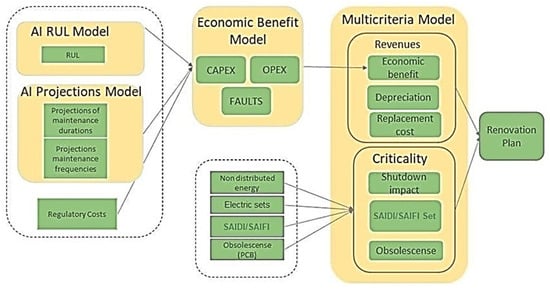
Figure 1.
Data flow for the analytical tool FERA [authors].
As it can be seen, there are five major groups of primary set data designed to produce the asset renovation or replacement plan:
- The first group consists of three categories of primary input data, namely: RUL data calculated by an artificial intelligence model, projections of maintenance durations and frequencies also calculated by an intelligence model, and regulatory costs.
- The second group, obtained from the previous group, defines the economic benefit model which, in its turn, helps define capital expenditure (CAPEX) and operational expenditure (OPEX) data, together with data from faults.
- The third group is composed of data from non-distributed energy, electric sets, SAIDI/SAIFI (system average interruption duration index/system average interruption frequency index), and obsolescence. SAIDI and SAIFI are two quality indicators of electrical energy system service provided.
- The second and the third groups are inputs for the fourth group that defines the revenue group, composed of data from the economic benefit model, as well as depreciation and replacement cost data.
- The fifth group defines the criticality group, which, in its turn, is composed of data from shutdown impact, SAIDI/SAIFI set, and obsolescence.
- Finally, the fourth and fifth groups contribute to the sixth group, which is the multicriteria model designed to provide the method for choosing which kinds of assets match the renovation plan.
3.1. New Maintenance Projection Models
In this work, two new ML models for maintenance projection were developed, with five general variables related to system equipment, namely manufacturer, regional office, family, age, and RUT.
One of the ML models was devoted to the frequency of corrective maintenance, while the other to the frequency of preventive maintenance. It was also decided to use frequency variables for corrective and preventive maintenance as input data for the corrective maintenance model, considering that the occurrence of preventive maintenance could have an impact on that of corrective maintenance. So, variables of the two types of maintenance were used for the preventive maintenance frequency projection model.
Once the variables had been defined, a Random Forest Algorithm [26] was used to generate the maintenance frequency models. The Random Forest Algorithm was chosen because it provided the smallest average error among the evaluated models. These models were trained using 10-fold cross-validation [27] and real databases containing more than ten thousand pieces of equipment used for training ML models. In addition, the models were implemented considering a database with the frequency of maintenance in the years 2016–2018, to make a forecast for the years 2019 and 2020. However, for the general context of this work, it was also necessary to extend the forecast for the equipment until the end of its useful life, which is commonly longer than 30 years. This time window for a ML algorithm implies a greater margin of prediction error.
Thus, two approaches were carried out to project the frequency of maintenance until the end of useful life. The first, called “incremental approach”, used the same ML model generated for projection to the years 2019 and 2020, changing only the input database. For this database, if the equipment did not reach an age equal to or greater than the RUL, the “equipment age” field was changed, increasing with each interaction. For example, for the year 2020, a given piece of equipment was 30 years old and had a RUL equal to 34 years.
To calculate the 2021 projection for the given equipment, the same variables as the previous year were used, except for the age plus one, which was equal to 31 years. Once this operation was carried out, the new base was used as an input to predict the maintenance frequency for this year. Similarly, for the year 2022, the age of this equipment was equal to 32 years, and the same ML model was used for this year’s projection, this procedure being repeated until the equipment reached the end of its useful life (34 years). This approach used a single ML model for all temporal projections, thus avoiding the generation of specific ML models every year, a process that would have implied higher computational cost.
However, aiming at more accurate results, a second approach, called feedback, was proposed, in which, given a base of entry, a new ML model was generated each year, changing two variables of the database used as input, i.e., (i) the age of the equipment (similarly to the first approach) and (ii) the maintenance frequency of the years prior to the desired projection, to be calculated from a feedback system.
This process was carried out repeatedly until all equipment reached its estimated useful life. This feedback system was obtained based on the frequency of three years prior to the desired projection, being divided into two steps. In the former, the maintenance frequency of 3 years was used to project the fourth year. For example, data from the 2016–2018 period were used to project the year 2019, this year being the output of the ML model. In the latter step, the maintenance frequency of the first year was eliminated from the system, and the maintenance frequency of the year projected prior to the third year was added. For example, to project the maintenance frequency in the year 2020, the frequency of the year 2016 was eliminated and the year 2019 was added.
Similarly, the process was carried out for the remaining years until the useful life of the equipment was exceeded. In this approach, for each feedback a new ML model was generated. In addition, this approach allowed combining the maintenance frequencies generated by the model and updated data (e.g., files with the maintenance that occurred in the years 2020–2024), generating new and more precise projections. The entire process was carried out automatically, and results were available in an output file containing three fields: equipment number, year, and maintenance frequency projected to this year.
Finally, the projection for the duration of frequencies was calculated, which was also part of the general scope of the project as illustrated in the data flow of Figure 1. To obtain this projection of maintenance duration, the average duration for each RUT was calculated from the sum of three variables: proportional planning, proportional displacement, and man-hour (M × H).
3.2. Financial Evaluation Models
Part of the criteria used to characterize the equipment to be assessed was related to the revenues or costs that they generated for the company. The indicators that quantified the CAPEX and OPEX values of the equipment were then treated. The CAPEX of an asset, which is considered as revenue that the equipment generates for the company, was obtained from its regulatory remuneration, with base values of gross and net remuneration being defined for each regulatory tariff cycle.
In one of the steps of this work, it was necessary to correlate the remuneration values from two different databases of the company. In this way, it was possible to obtain gross and net remuneration values for each equipment and then the regulatory reintegration share (RRS) (Equation (1)) and net capital remuneration (NCR) (Equation (2)) for each tariff regulatory cycle:
where GRB is the gross remuneration base, which comprises the new value replacement (NVR) of the set of assets and installations of the company. NRB is the net remuneration base, δ is a variable representing the depreciation average rate of an asset, and WACC is the weighted average cost of capital.
RRS = GRB × δ
NCR = NRB × WACC
Figure 2 shows the input variables for obtaining the equipment revenue parameter indicated by its net present value: NVR, accumulated depreciation (the total amount an asset has been depreciated up until a single point), depreciation rate (the percentage rate at which an asset is depreciated across the estimated productive life of the asset), WACC, regulatory lifetime (lifetime of an asset determined by regulatory agencies), and yechnical useful life (lifespan of a depreciable fixed asset, during which it can be expected to contribute to company operations).

Figure 2.
Variables used for calculating revenue via the net present value (NPV) [authors].
The OPEX of the asset was quantified based on the costs of preventive and corrective maintenance, considering the results of machine learning algorithms for the projection of maintenance frequencies. The cost that the distributor will incur with this equipment, until the end of its technical useful life, was obtained from projections, average maintenance duration for each RUT, and cost of M × H from the company. Figure 3 shows inputs and outputs for this model: cost: M × H, M × H, propose_planning (asset’s planned commissioning date), propose_displacement (postponement of the date of entry into operation of the asset), frequency (maintenance frequency), and technical useful life.
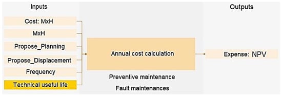
Figure 3.
Variables for calculating equipment operating costs [authors].
Finally, for each piece of equipment (e,p), the aggregate gain, also called economic benefit, was obtained as the difference between income and expenses in the present value (Equation (3)):
Gaine,p = CAPEXe,p − OPEXe,p
3.3. Multicriteria Models
The analytic hierarchy process (AHP) method is among the most used to analyze decision making based on multiple criteria [28,29]. It is a simple method that allows one to select the best options among several different alternatives using qualitative and quantitative parameters.
By this method, a comparison of the parameters under analysis was performed, using weights established by the planner. After determining the critical criteria, assigning weights, and comparing these multiple criteria, the priority alternative was found within a set of options. It also provided clear reasoning on why such an alternative is the best.
The AHP method consists of three phases: (1) structuring, (2) judgement, and (3) synthesis of the results. The first structuring phase consists of producing the decision model, which is presented as a hierarchy. There are two types of structuring, i.e., bottom-up and top-down. The bottom-up type structuring, which is used when the alternatives are better understood than the objectives, has three steps, i.e., (a) identifying the alternatives, (b) listing the pros and cons of each alternative, and (c) obtaining the criteria and objectives from the decision of the pros and cons. The top-down type one, which is preferable for strategic decisions where the objectives are better understood than the alternatives, also has three steps, i.e., (a) obtaining the main objective(s) of the decision, (b) identifying the secondary objectives, criteria, sub-criteria, etc., and (c) grouping alternatives at the last hierarchical level. Forman and Gass [30] established a numerical scale for determining the weights of the criteria to be adopted.
In the next phase of judgement, elements of the same hierarchical level must be compared with each other. From psychological experiments, it was discovered that the human brain has a limit for simultaneous comparisons of about 7 ± 2 items, i.e., a maximum of 9 [29]. Thus, the number nine appears as a limit to the number of elements per hierarchical level. After the decision model was structured, the next phase of the AHP was the judgment by specialists. Figure 4 exemplifies the steps of the method.

Figure 4.
Flowchart for application of the AHP method, CR—consistency ratio. Adapted from Saaty [30].
Finally, the last phase of the AHP method consists of obtaining and analyzing the results. This method can be summarized by the following steps: (1) definition of the problem and what criteria will be applied, (2) construction of the hierarchical decision structure, (3) construction of matrix for judging criteria, (4) calculation of local average priorities, (5) construction of the judgment matrix of the alternatives, based on a peer-to-peer comparison, and (6) calculation of global priorities.
In the field of energy distribution, studies such as those of Saaty [30] and Mussoi [31] used this method in prioritizing investments. Figure 5 schematizes the hierarchical decision tree for analysis at two levels of hierarchy aiming at prioritizing equipment exchange using the AHP method.
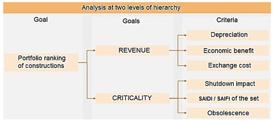
Figure 5.
Hierarchical decision tree for this work [authors].
3.4. Remaining Useful Life Estimation Model: Training and Testing
The RUL can be estimated by calculating the difference between the technical useful life (TUL) and the age of the asset. As can be seen in Figure 6, nine variables were used as inputs to estimate the RUL. The TUL value for each asset was obtained through a regression task performed by ML models. Altogether, four ML algorithms were used, namely Random Forest [32], multiple linear regression [33], decision tree [34], and gradient boosting [35].
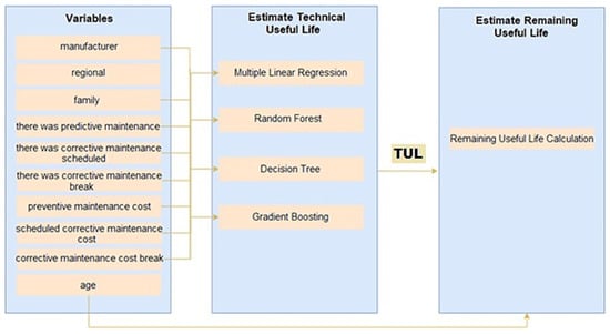
Figure 6.
Main methodological flow for estimation of the RUL [authors].
In this context, the decision tree and Random Forest algorithms were chosen considering the possibility of visualizing the rules formed by them to estimate the RUL, making it possible to analyze the learning according to the variables shown in Figure 6. In addition, the option of the gradient boosting was selected thanks to its ability of displaying, on a scale from 0 to 1, the importance of each variable for the trained model.
Finally, a simplified model was trained by multiple linear regression, since the others are ML algorithms of greater computational complexity and, consequently, tend to over-adjust the model for simpler tasks. Based on this procedure, for each RUT, training and validation of the model were carried out through three main steps (Figure 7): (a) pre-processing, (b) estimation of the RUL via ML model, and (c) analysis of variables and errors.
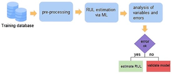
Figure 7.
Training and validation of the RUL model estimation for each RUT [authors].
Training and testing databases were obtained through an ETL (extraction, transformation, and loading) process. Several databases from various corporate systems were used. Section 4.2 provides more information.
As pre-processing, the TUL (used as a label for the training base) and the cost variables were normalized on a scale of 0 to 1 and discretized by the Quantile Method [36], respectively. In addition, for the manufacturer variable the manufacturer’s name was replaced by the manufacturer’s average TUL based on two rules: (1) if there were more than ten pieces of equipment from a manufacturer in the training base, the name of the equipment was replaced with its average TUL; (2) otherwise, it was replaced with the average TUL of all manufacturers available on the training base.
These manufacturer rules were applied to help the ML model to generalize cases in which there were minority manufacturers in the base (i.e., they have a small number of samples), as well as future prediction (i.e., in test bases) of equipment whose manufacturers do not exist in the training base. In addition, the database contains primary and secondary equipment.
After pre-processing, the RUL estimation stage was performed via ML in which each model was trained. So, the training was carried out using cross-validation of four machine learning models, one for each algorithm illustrated in Figure 6. In the cross-validation, a total of five folds were used (we set k = 5 to keep a compromise between computational cost, bias, and variance), in which the result was obtained for each fold. The error between the TUL estimated by the algorithm and the original TUL (label) of the training base was calculated using the mean absolute error (MAE) metric.
With the trained models, the TUL of each one was estimated to analyze the variables and errors obtained. In the analysis of variables, the rules of the decision tree and Random Forest models were visualized; then, the error, extracted using the MAE, was analyzed. When the model gave results below ten years, the RUL was estimated through the difference between the age and the TUL of the equipment. When the model returned an error over ten years, the previous steps were resumed to validate the model.
After this stage, the same pre-processing was applied to the test base, and the RUL was estimated through the trained algorithms. This base represents equipments that are active and, consequently, do not have a real TUL label. Therefore, instead of calculating the MAE to analyze the results, a statistical analysis was performed to identify possible errors in the ML models. The flow applied to the test base is illustrated in Figure 8.
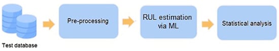
Figure 8.
Testing of the RUL model estimation for each RUT [authors].
As shown in Figure 7 and Figure 8, the models were trained using a training base, and the RUL was estimated on a test base. Therefore, for the training base, some equipment was removed from the handling base, and those in the scrap or “warehouse Z” (name given to the company assets removed from operation) were used for training. Then, the TUL was estimated for all existing equipment not included in the warehouse or scrap. In all, the TUL was estimated for 14 RUTs, so 14 machine learning models were trained for each type of approach, i.e., Random Forest, decision tree, regression, and gradient boosting (XGBoost). The models were trained with cross-validation using the MAE metric, as previously described. The MAE, obtained using Equation (4) below, was used to calculate the proposed model error on a scale of years. This scale was evaluated considering that for the model to be validated, it must obtain an error of at least half of the value of the average regulatory useful life of the RUT, which is a pre-defined criterion by RUL specialists from COPEL.
where n is the total number of equipments and |u − û| is the difference between the actual technical lifetime and the technical lifetime predicted by the proposed model. Table 1 lists the MAE for each model and RUT, using a training base.

Table 1.
Performance of ML algorithms by RUT.
To understand and identify possible problems, a case study was carried out of the RUT 570 (power transformer), which presents a larger amount of data and a higher proportion between renewal classes. The Random Forest algorithm was chosen because it provided the smallest average error among the evaluated models; therefore, the analysis presented in the following section contemplates the results of the predictors using this algorithm.
4. Results
This section shows the applications and results of the ML models chosen to estimate the RUL, as well as the projection of maintenance, applied to the electric sector, specifically to the assets of the Brazilian energy distributor COPEL. The results obtained from the application of this research in a case study is presented and discussed. Additionally, the asset renewal tool software (FERA) is presented through its architecture and some screenshots.
4.1. Application in the Brazilian Electric Sector
As the result of this research deals with methodology and software, the verification of functionality was carried out through a test of use and comparison of case study results with renovation plans available. The initial proposal for validating the results was the comparison of a renewal of assets elaborated with the current methodology of COPEL and with the asset renewal tool developed in this work.
Next, the step-by-step preparation of the decision model proposed in this work was performed, with analytical descriptions of the results obtained considering assets from RUT 570. Figure 5 highlights the two levels of hierarchy used, characterized by two objectives and three judgment criteria for each objective. For the results that are presented below, the evaluation of the objectives and default criteria were considered according to the judgment matrices shown in Table 2, Table 3 and Table 4.
Table 2.
Objectives judgment matrix.
Table 3.
Judgment matrix of revenue criteria.
Table 4.
Judgment matrix of criticality criteria.
The values listed in these tables were obtained from a prioritization study of substation assets carried out using indicators obtained from RUL projection reports and maintenance frequency projections until the end of their (substation assets) TUL. These reports were generated by the FERA tool.
It is important to remember that by the very definition of the model, all judgment matrices are reciprocal (aij = aji) and can be reconstructed with an amount of elements less than n2, where n is the dimension of the matrix. In fact, for the matrices in question, all relations were completely described by seven input values (Table 5).
Table 5.
Description of the AHP model weights database in this work.
For each of the matrices in Table 3, Table 4 and Table 5, the maximum eigenvalues were calculated (via product of an auxiliary matrix with the normalized eigenvector), as well as the coherence indices and the ratios of consistency, following the AHP method. The normalized eigenvectors of the criteria matrices and the goals matrix were multiplied to assign the average local priorities (or global weights), shown in Table 6.
Table 6.
Global weights of the AHP model considering default judgment.
These global weights were applied to the alternatives (RUT 570 equipment) to establish global priorities. For each of the evaluated criteria, the attributes listed in Table 7 were used.
Table 7.
Equipment attributes used to establish global priorities.
Once the attributes were obtained, it was necessary to make the relationship between them coherent, i.e., to rank the equipment by exchange priority, assets with higher GPC, obsolescence levels, shutdown impacts, and depreciation rates, as well as the lowest switching costs and economic benefit values. In this way, the inverse of the switching cost (1/NRV) and the opposite of economic benefit (−NPV) were used for ranking.
In addition, the attributes were normalized to obtain comparisons on the same scale using the max–min strategy (Equation (5)), which restricts the values in the range from zero to one:
Thus, for example, a completely depreciated asset has a depreciation criterion equal to the unit and equipment located in the set with the smallest GPC has null SAIDI/SAIFI criterion.
Table 8 lists the maximum and minimum values of each of the criteria before the normalization.
Table 8.
Maximum and minimum values of the evaluated attributes.
After normalization, the attribute values of each asset were multiplied by the weights of the criteria. The aggregate of these products resulted in a global score for each equipment, allowing the ranking. A priori, the maximum possible score was one.
From the clipping carried out, it became evident that the equipment exchange prioritization model developed highlighted the accumulated depreciation (EAD) and the economic benefit (−NPV) as factors of greater importance for the ranking, since all the assets presented in Table 7 have EAD and −NPV values normalized close to unity. This effect can also be observed by the dispersion of scores relating to normalized depreciation and economic benefit installments (40.36% × EAD + 16.34% × (−NPV)) with respect to the global score of the assets, which can be approximated by a straight line with R2 = 0.9869 (Figure 9).
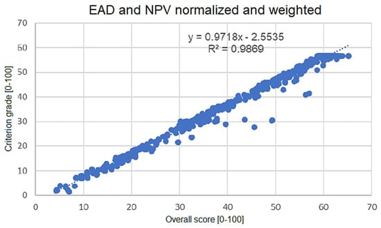
Figure 9.
Dispersion of scores relating to the accumulated depreciation and benefit criteria weighted against global scores [authors].
It should be noted that 116 of the 563 assets analyzed were completely depreciated according to data from the 2019 ACR, which was graphically identified by the plateau in Figure 9 for the highest global grade equipment. The distribution of the normalized accumulated depreciation of the assets can be viewed by the histogram shown in Table 9 and Figure 10.
Table 9.
Accumulated asset depreciation histogram data.
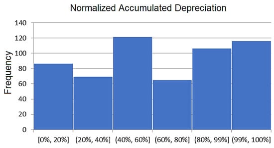
Figure 10.
Histogram of accumulated asset depreciation [authors].
Thus, with a rather depreciated base, it was up to the other criteria to determine the ordering of asset exchange priority. According to the data listed in Table 6, the global weights of the other criteria, in descending order, were the following: impact of shutdown (17.27%), exchange cost (15.13%), SAIDI/SAIFI (7.48%), and obsolescence (3.43%).
Figure 11 shows the dispersion of scores (without weighting, that is, ranging from 0 to 100 and not limited to criterion weight) of each of the above four criteria with respect to the global score. To characterize the tiebreaker between the first placed, the analysis was limited to the first 134 assets, position occupied by the last fully depreciated asset.
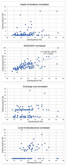
Figure 11.
Dispersion of assets when individualized criteria were evaluated [authors].
As can be seen by combining the depreciation and economic benefit scores, there is no direct relationship between individual criteria and overall score. For SAIDI/SAIFI, the criterion with greatest adherence to linear behavior, R2 = 0.5238, was calculated. It is worth mentioning the concentration of assets with very low scores for some criteria, even in the first places, which indicates the existence of extreme values that distort the max–min normalization, not compromising, however, the established priority list.
Still maintaining the restriction to the first 134 assets, the effect of the composition of the four criteria for the ordering of equipment can be seen in Figure 12, with good linear approximation (R2 = 0.8804). Therefore, the combination of criteria was essential to obtain the desired ordering.

Figure 12.
Dispersion of assets when evaluated combined criteria [authors].
In summary, the established AHP model was developed for determining exchange priority of RUT 570 equipment. Applying the AHP methodology, the results of questionnaires with COPEL’s technical staff were used to determine the weights of six evaluation criteria (depreciation, economic benefit, exchange cost, shutdown impact, SAIDI/SAIFI, and level of obsolescence), composing revenue and criticality objectives.
The results in Table 8 indicate the strong incidence of depreciation and economic benefit as priority criteria, which is reinforced by the dispersion shown in Figure 9. In other terms, considering the determined weights, it is possible to establish a preliminary ranking based solely on depreciation and economic benefit that is faithful to the prioritization based on the six criteria.
On the other hand, the weighting of the four other criteria was necessary for the purposes of a tiebreaker. In this regard, it is noteworthy that there was no individual criterion capable of capturing the effect of composition of all plots (Figure 11), it being essential that there be a joint final assessment to obtain the proposed ranking (Figure 12).
4.2. Experiments Using Incremental and Feedback Approaches
As a way of evaluating the results obtained from the application of the incremental and feedback approaches, two case studies were carried out for RUTs 210 (circuit breaker) and 340 (voltage regulator) in the year 2019 regarding the frequency of corrective maintenance (Figure 13). For these RUTs, the corrective maintenance model allowed projecting an average maintenance frequency carried out that year of around 0 and 0.5.
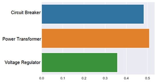
Figure 13.
Average maintenance frequency predicted for 2019 [authors].
4.2.1. Case Study: RUT 210 (Circuit Breaker)
Initially, the distribution of data from the training and test bases was analyzed to identify discrepancies. In this regard, for both cases, costs and RUT had a similar average between the bases, although the average age was different between the two bases. A comparison of the age distribution in the test base with that in the training one (Figure 14) shows that most equipment in the former was new, aging up to 20 years, while a high amount of the one in the latter was more than 30 years old.
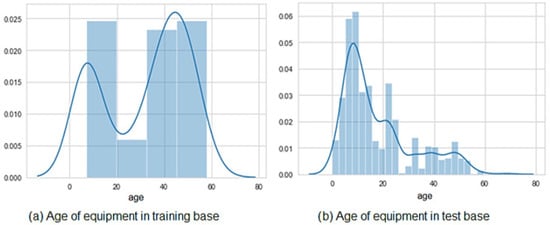
Figure 14.
Age of equipment in the (a) training and (b) test bases [authors].
Since the two bases are differentiated mainly by the age of the equipment, the RUL estimated by the random forest predictor and the age of the equipment in the test base are correlated in Figure 15. As can be seen, the predictor estimated that, in general, most equipment under the age of 31 years was still within the estimated useful life, contrary to the older one.
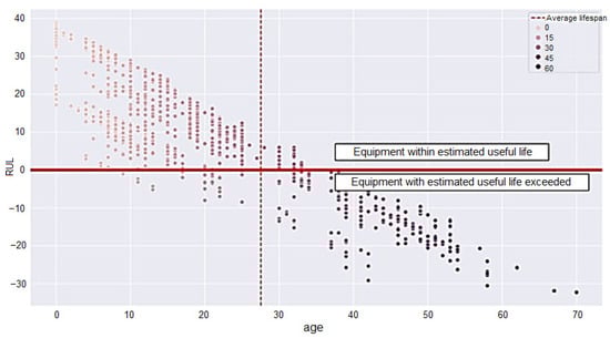
Figure 15.
Relationship between the estimated useful life and the age of the equipment for RUT 210 [authors].
This result is justified by the training base, given that the average useful life of the Siemens equipment is around 15 years. Consequently, it can be said that the predictor created specific decision rules for this manufacturer, so that, when viewing new data from it, the useful life of the equipment was also estimated at around 15 years. In addition, it was identified that the test base and training base have some different manufacturers. However, the predictor did not distinguish the equipment as to the manufacturer’s existence in the training base, thus validating the pre-processing performed for this attribute.
4.2.2. Case Study: RUT 340 (Voltage Regulator)
Likewise, data distribution and remaining life estimation were performed for the RUT 340. Just as for the RUT 210, the average age was a differential between the bases. Figure 16 illustrates the distribution of equipment according to age, on a scale from zero to one. Therefore, as in the previous case study, the two bases have different distributions for this attribute.

Figure 16.
Age of equipment in the training and test bases for the RUT 340 [authors].
Figure 17 illustrates the corresponding relationship between the estimated useful life and age. The average service life of the manufacturers of the training base was less than or equal to 20 years, which indicates that the predictor, as for RUT 210, created specific rules based on the manufacturers.
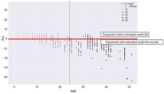
Figure 17.
Relationship between the estimated useful life and the age of the equipment for RUT 340 [authors].
Finally, based on the analysis showed in this section, it was observed that, in general, for both RUTs, the machine learning algorithm can estimate the RUL for equipment that is below or equal to the average age of the equipment. Above the average age, the predictor identifies the equipment as an outdated service life. In addition, it was observed that, although the predictor estimates the useful life of all equipment in general, the equipment from manufacturers that had a lower average useful life were generalized by the predictor and considered as an outdated useful life.
4.3. Asset Renewal Tool Architecture
Figure 18 shows an overview of the final proposed architecture for the FERA software. Following the flow of data entry to the view of the dashboard by users, the tool has the following basic architectural elements:
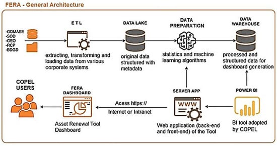
Figure 18.
Overview of the architecture of the FERA [authors].
- Extraction, Transformation, and Loading (ETL) module. It is responsible for ingesting data from the various corporate systems that are used by the tool, namely GDMASE (a substation maintenance system), SOD (a distribution operation system), GEO (a geographic information system), RCP (acronym for Relatório de Controle Patrimonial in Portuguese, meaning asset control report), and BDGD (acronym for Base de Dados Geográficos da Distribuidora in Portuguese, meaning distributor geographic database). In this module, the metadata of each available data set are identified and transferred to the Data Lake;
- Data Lake. It is a structured data repository with metadata (name, size, type, etc.) arranged in a database from which access and necessary combinations between different information are allowed;
- Data Preparation. It is a module responsible for executing queries, transforming data, and executing statistical and ML algorithms on data from the Data Lake to obtain indicators and structured data for the generation of dashboards;
- Data Warehouse. It is a structured data repository to generate the tool’s dashboards, which consists of a database in the format of a data warehouse with easy data disposition for the use of business intelligence (BI) and data analysis tools;
- Power Business Intelligence. It is a BI tool adopted by COPEL for data analysis, construction of reports, and graphs, which is responsible for viewing data on the dashboard;
- Web Application Server. It is a Web application responsible for data configuration, integration of the Power BI tool and user interaction, which consists of the back-end and front-end (user interface) services that define the FERA software;
- Dashboard. It is a user interaction interface where graphical and tabular information on asset renewal indicators is presented. It also allows the configuration of system parameters and other tool administration actions.
4.3.1. Software Architecture
Figure 19 shows a view of the software architecture used to execute the components of FERA. The modules that make up the tool use a set of software that involves operating systems, programming languages, and data visualization tools. To make the tool available in the “on premises” format, that is, using COPEL’s information technology (IT) infrastructure, it was necessary to license some software in accordance with corporate standards:
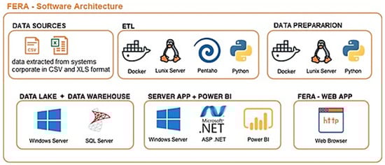
Figure 19.
View of the software architecture used to execute the components of the FERA [authors].
- Data Sources. Data are made available in CSV (comma-separated values) format and may also be made available in XLSX format (Excel spreadsheet) or another format according to the need;
- ETL Module. It uses Python scripts and programs combined with Pentaho Kettle scripts to extract data and send them to the Data Lake. These programs are run on Linux operating systems with an environment configured from a Docker container;
- Data Preparation Module. It uses scripts and programs in Python language executed on Linux operating system with an environment configured from a Docker container;
- Data Lake and Data Warehouse modules. They consist of databases using the Microsoft SQL Server Database Management System (DBMS) running on the Microsoft Windows Server operating system;
- Application Server Module. It consists of a Web application developed under the Microsoft ASP.NET platform and the Microsoft Power BI tool, running on the Microsoft Windows Server operating system. In this module, Windows Server licensing is required. Licensing of the Power BI tool is not mandatory, and the desktop version can be used free of charge by Microsoft;
- Asset Renewal Tool. It is a common Web application that can be run on the latest versions of available Internet browsers.
4.3.2. Hardware Architecture
Some components of the presented infrastructure are made available within COPEL’s server configuration, such as the database server and the Web application server. The values for processing capacity, memory, and storage were based on the cloud infrastructure used for the development of the tool. Figure 20 shows a view of the hardware architecture used to execute the components of the FERA.

Figure 20.
View of the hardware architecture used to execute the components of the FERA [authors].
The tool was developed using a cloud architecture where the hardware infrastructure and network services are configured in a more flexible way, allowing their adaptation in a more simplified way. To make the tool available in the ”on premises” format, it was necessary to configure the hardware infrastructure by COPEL’s IT area. The hardware components for running the tool are:
- File Server. It is a repository of files to be extracted for the tool. The data extracted from the corporate systems are made available on a share on a COPEL file server, with read permissions for a user specially created for the ETL module;
- Workstations for users to use the tool. They have no specific configuration, and may be desktop computers or laptops using Windows, Linux, or MacOS operating systems with sufficient processing and memory to run Internet browsers;
- Asset Renewal Tool modules. They can be executed on physical or virtualiz servers with access between them within COPEL’s corporate network. Table 10 shows the hardware infrastructure needed to execute the module that makes up the asset renewal tool.
Table 10. Hardware infrastructure.
5. Conclusions
This paper presented an overview of the most relevant results obtained from the development and application of a new methodology to support decision making and a tool for planning actions for the maintenance and replacement of assets using advanced techniques from data analytics. The FERA software is being used by the Companhia Paranaense de Energia (COPEL), one of the largest energy distribution companies in the southeast region of Brazil.
After a brief contextualization and presentation of the problem to be dealt with, the paper presented a brief review of the literature related to RUL prediction of engineered systems. For the development of this work, a broad methodology was set up comprising distinct but interrelated models, which have been presented and discussed in this paper as the proposed solution, i.e., a concurrent multicriteria model, a model for the maximization of asset value across its life cycle, a model for simultaneously weighting remuneration rules and quality of service from the current regulation framework, a risk analysis as a function of adopted decisions, and actions.
Next, the paper presented the experiments conducted during the research and the results obtained by applying the designed methodology to one case study (RUT 570—power transformer). In this regard, the obtained results showed that considering the determined weights, it is possible to establish a preliminary ranking (of equipment by exchange priority) based solely on depreciation and economic benefit that is faithful to the prioritization based on the six criteria. Additionally, there is no individual criterion capable of capturing the effect of composition of all plots, it being essential that there is a joint final assessment to obtain the proposed ranking.
Finally, the paper presented an overview of the final proposed architecture for the FERA software.
6. Future Work
The research presented in this paper has the potential to be extended to other related areas. This can be inferred from the presence of RUL estimation works in industries not related to electricity. For example, Lei and Sandborn [37] and Sivalingam et al. [38] reported RUL prediction methods in the wind energy scenario. The predictive model described in this paper can assist in the management of plant resources.
Author Contributions
Conceptualization: H.d.C.S., M.H.d.N.M., J.C.d.S.C. and R.B.C.P.; methodology: H.d.C.S., M.H.d.N.M., J.C.d.S.C. and R.B.C.P.; software: H.d.C.S., J.C.d.S.C. and R.B.C.P.; validation: H.d.C.S., J.C.d.S.C. and R.B.C.P.; formal analysis: H.d.C.S., M.H.d.N.M., J.C.d.S.C. and R.B.C.P.; investigation: H.d.C.S. and J.C.d.S.C.; resources: H.d.C.S. and M.H.d.N.M.; writing—original draft preparation: H.d.C.S., M.H.d.N.M., J.C.d.S.C. and R.B.C.P.; writing—review and editing: M.A.M., L.A.S. and A.C.; visualization: H.d.C.S.; supervision: L.A.S., A.C. and M.H.d.N.M.; project administration: M.H.d.N.M.; funding acquisition: H.d.C.S. and M.H.d.N.M. All authors have read and agreed to the published version of the manuscript.
Funding
This work received funding and technical support from COPEL (Companhia Paranaense de Energia) as part of the ANEEL PD-02866-0514/2019 project, “Tool to Support the Optimization of Asset Renewal Decisions”, which is part of an R and D program regulated by ANEEL, Brazil. Coordination for the Improvement of Higher Education Personnel—Brazil (CAPES)—Financing Code 001.
Data Availability Statement
Not applicable.
Acknowledgments
This work was partially supported by the Brazilian agency CAPES and Brazilian National Council for Scientific and Technological Development (CNPq), process number 310862/2022-1. The authors thank the Systems Engineering Program at Polytechnic School, University of Pernambuco (UPE), and the Brazilian companies In Forma Software and Sinapsis, for structural support. The authors also thank the researchers Ana Gabriela Bezerra Benitez (from University of São Paulo, USP), Cecília Flávia da Silva, and Starch Melo de Souza (from Informatics Center, Federal University of Pernambuco, UFPE) for their support to the experimental work.
Conflicts of Interest
The authors declare no conflict of interest.
Abbreviations
RUL—remaining useful life; RAV—replacement asset value; PHM—prognostics and health management; ML—machine learning; RUT—register unit type; CAPEX—capital expenditure; OPEX—operational expenditure; SAIDI/SAIFI—system average interruption duration index/system average interruption frequency index; RRS—regulatory reintegration share; NCR—net capital remuneration; NVR—new value replacement; NRB—net remuneration base; WACC—weighted average cost of capital; AHP—analytic hierarchy process; TUL—technical useful life; MAE—mean absolute error; FERA—ferramenta para estimação de renovação de ativos, in Portuguese (tool for estimation of asset renewal, in English); COPEL—Companhia Paranaense de Energia.
References
- Mattos Neto, P.; Oliveira, J.; Domingos, S.; Siqueira, H.; Marinho, M.; Madeiro, F. An adaptive hybrid system using deep learning for wind speed forecasting. Inf. Sci. 2021, 581, 495–514. [Google Scholar] [CrossRef]
- Sial, A.; Singh, A.; Mahanti, A. Detecting anomalous energy consumption using contextual analysis of smart meter data. Wirel. Netw. 2021, 27, 4275–4292. [Google Scholar] [CrossRef]
- Sial, A.; Singh, A.; Mahanti, A.; Gong, M. Heuristics-Based detection of abnormal energy consumption. In Smart Grid and Innovative Frontiers in Telecommunications. SmartGIFT 2018. Lecture Notes of the Institute for Computer Sciences, Social Informatics and Telecommunications Engineering; Chong, P., Seet, B.C., Chai, M., Rehman, S., Eds.; Springer: Cham, Switzerland, 2018; Volume 245, pp. 21–31. [Google Scholar] [CrossRef]
- Si, X.-S.; Wang, W.; Hu, C.-H.; Zhou, D.-D. Remaining useful life estimation—A review on the statistical data driven approaches. Eur. J. Oper. Res. 2011, 213, 1–14. [Google Scholar] [CrossRef]
- Akpan, J.; Olanrewaju, O.A. Asset management models brief review and framework development for energy sustainability & sustainable development. In Proceedings of the International Conference on Industrial Engineering and Operations Management, Istanbul, Turkey, 7–10 March 2022; pp. 1229–1239. [Google Scholar]
- Cavalcanti, G.; Feitosa, M.; Pereira, K.; Marinho, M.; Neto, A.; de Carvalho Sobral, L.; Goncalves, P.M.R.; Lara, D.T.M.; Gomes, T.F.; Teixeira, R.J.; et al. Efficiency of class III surge protection devices against lightning surges. IEEE Lat. Am. Trans. 2021, 19, 1459–1467. [Google Scholar] [CrossRef]
- Olesen, J.F.; Shaker, H.R. Predictive maintenance for pump systems and thermal power plants: State-of-the-art review, trends and challenges. Sensors 2020, 20, 2425. [Google Scholar] [CrossRef]
- Li, W.; Vaahedi, E.; Choudhury, P. Power system equipment aging. IEEE Power Energy Mag. 2006, 4, 52–58. [Google Scholar] [CrossRef]
- Omer, A.M. Energy, environment and sustainable development. Renew. Sustain. Energy Rev. 2008, 12, 2265–2300. [Google Scholar] [CrossRef]
- Izidio, D.; Mattos Neto, P.; Barbosa, L.; Oliveira, J.; Marinho, M.; Rissi, G. Evolutionary hybrid system for energy consumption forecasting for smart meters. Energies 2021, 14, 1794. [Google Scholar] [CrossRef]
- Mattos Neto, P.; Oliveira, J.; Bassetto, P.; Siqueira, H.; Barbosa, L.; Alves, E.; Marinho, M.; Rissi, G.; Li, F. Energy consumption forecasting for smart meters using extreme learning machine ensemble. Sensors 2021, 21, 8096. [Google Scholar] [CrossRef]
- Meng, J.; Yue, M.; Diallo, D. A degradation empirical-model-free battery end-of-life prediction framework based on Gaussian process regression and Kalman filter. Trans. Transp. Electrif. 2022. [Google Scholar] [CrossRef]
- Johnstone, D.J. Replacement cost asset valuation and regulation of energy infrastructure tariffs. Abacus 2003, 39, 1–41. [Google Scholar] [CrossRef]
- Companhia Paranaense de Energia S.A.-Copel. Available online: https://www.copel.com/site/institucional/nossa-historia/ (accessed on 27 February 2023).
- Agência Nacional de Energia Elétrica. Available online: https://www.gov.br/aneel/pt-br (accessed on 27 February 2023).
- Shearer, C. The CRISP-DM model: The new blueprint for data mining. J. Data Warehous. 2000, 5, 13–22. [Google Scholar]
- Predictive Maintenance Toolbox. Available online: https://www.mathworks.com/products/predictive-maintenance.html (accessed on 27 February 2023).
- Liao, L.; Köttig, F. Review of hybrid prognostics approaches for remaining useful life prediction of engineered systems, and an application to battery life prediction. IEEE Trans. Reliab. 2014, 63, 191–207. [Google Scholar] [CrossRef]
- Li, S.; Ma, H.; Saha, T.K.; Yang, Y.; Wu, G. On particle filtering for power transformer remaining useful life estimation. IEEE Trans. Power Deliv. 2018, 33, 2643–2653. [Google Scholar] [CrossRef]
- Catterson, V.M. Prognostic modeling of transformer aging using Bayesian particle filtering. In Proceedings of the 2014 IEEE Conference on Electrical Insulation and Dielectric Phenomena (CEIDP), Des Moines, IA, USA, 19–22 October 2014; pp. 413–416. [Google Scholar] [CrossRef]
- Walsh, T.R.; Alhloul, S.; Hajimorad, M. Estimating the remaining useful life of power grid transmission lines using synchrophasor data. In Proceedings of the 2014 International Conference on Prognostics and Health Management, Cheney, WA, USA, 22–25 June 2014; pp. 1–8. [Google Scholar] [CrossRef]
- Mosallam, A.; Medjaher, K.; Zerhouni, N. Data-driven prognostic method based on Bayesian approaches for direct remaining useful life prediction. J. Intell. Manuf. 2016, 27, 1037–1048. [Google Scholar] [CrossRef]
- Ragab, A.; Ouali, M.; Yacout, S.; Osman, H. Remaining useful life prediction using prognostic methodology based on logical analysis of data and Kaplan–Meier estimation. J. Intell. Manuf. 2016, 27, 943–958. [Google Scholar] [CrossRef]
- Elsheikh, A.; Yacout, S.; Ouali, M.S. Bidirectional handshaking LSTM for remaining useful life prediction. Neurocomputing 2019, 323, 148–156. [Google Scholar] [CrossRef]
- Zhang, C.; Lim, P.; Qin, A.K.; Tan, K.C. Multiobjective deep belief networks ensemble for remaining useful life estimation in prognostics. Trans. Neural Netw. Learn. Syst. 2016, 28, 2306–2318. [Google Scholar] [CrossRef]
- Kang, Z.; Catal, C.; Tekinerdogan, B. Remaining useful life (RUL) prediction of equipment in production lines using artificial neural networks. Sensors 2021, 21, 932. [Google Scholar] [CrossRef]
- Refaeilzadeh, P.; Tang, L.; Liu, H. Cross-validation. In Encyclopedia of Database Systems; Liu, L., Özsu, M.T., Eds.; Springer US: New York, NY, USA, 2009; Volume 5, pp. 532–538. [Google Scholar]
- Golden, B.L.; Wasil, E.A.; Harker, P.T. The Analytic Hierarchy Process: Applications and Studies, 1st ed.; Springer: Berlin/Heidelberg, Germany, 1989; Volume 2. [Google Scholar]
- Forman, E.H.; Gass, S.I. The analytic hierarchy process—An exposition. Oper. Res. 2001, 49, 469–486. [Google Scholar] [CrossRef]
- Saaty, T. Método de Análise Hierárquica; McGraw-Hill: São Paulo, Brazil, 1991. [Google Scholar]
- Mussoi, F.R.L. Modelo de Decisão Integrado para a Priorização Multiestágio de Projetos de Distribuição Considerando a Qualidade da Energia Elétrica. Ph.D. Thesis, Federal University of Santa Catarina, Florianópolis, Brazil, 2013. [Google Scholar]
- Livingston, F. Implementation of Breiman’s random forest machine learning algorithm. ECE591Q Mach. Learn. J. Pap. 2005, 1–13. [Google Scholar]
- Olive, D.J. Multiple linear regression. In Linear Regression, 1st ed.; Olive, D.J., Ed.; Springer: Cham, Switzerland, 2017; pp. 17–83. [Google Scholar]
- Tso, G.K.F.; Yau, K.K.W. Predicting electricity energy consumption: A comparison of regression analysis, decision tree and neural networks. Energy 2007, 32, 1761–1768. [Google Scholar] [CrossRef]
- Bentéjac, C.; Csörgő, A.; Martínez-Muñoz, G. A comparative analysis of gradient boosting algorithms. Artif. Intell. Rev. 2021, 54, 1937–1967. [Google Scholar] [CrossRef]
- Koenker, R. Quantile regression: 40 years on. Artif. Intell. Rev. 2017, 9, 155–176. [Google Scholar] [CrossRef]
- Lei, X.; Sandborn, P.A. Maintenance scheduling based on remaining useful life predictions for wind farms managed using power purchase agreements. Renew. Energy 2018, 116, 188–198. [Google Scholar] [CrossRef]
- Sivalingam, K.; Sepulveda, M.; Spring, M.; Davies, P. A review and methodology development for remaining useful life prediction of offshore fixed and floating wind turbine power converter with digital twin technology perspective. In Proceedings of the 2018 2nd International Conference on Green Energy and Applications (ICGEA), Singapore, 24–26 March 2018; pp. 197–204. [Google Scholar] [CrossRef]
Disclaimer/Publisher’s Note: The statements, opinions and data contained in all publications are solely those of the individual author(s) and contributor(s) and not of MDPI and/or the editor(s). MDPI and/or the editor(s) disclaim responsibility for any injury to people or property resulting from any ideas, methods, instructions or products referred to in the content. |
© 2023 by the authors. Licensee MDPI, Basel, Switzerland. This article is an open access article distributed under the terms and conditions of the Creative Commons Attribution (CC BY) license (https://creativecommons.org/licenses/by/4.0/).