Implementing Optimization Techniques in PSS Design for Multi-Machine Smart Power Systems: A Comparative Study

Abstract

This study performed a comparative analysis of five new meta-heuristic algorithms specifically adopted based on two general classifications; namely, nature-inspired, which includes artificial eco-system optimization (AEO), African vulture optimization algorithm (AVOA), gorilla troop optimization (GTO), and non-nature-inspired or based on mathematical and physics concepts, which includes gradient-based optimization (GBO) and Runge Kutta optimization (RUN) for optimal tuning of multi-machine power system stabilizers (PSSs). To achieve this aim, the algorithms were applied in the PSS design for a multi-machine smart power system. The PSS design was formulated as an optimization problem, and the eigenvalue-based objective function was adopted to improve the damping of electromechanical modes. The expressed objective function helped to determine the stabilizer parameters and enhanced the dynamic performance of the multi-machine power system. The performance of the algorithms in the PSS’s design was evaluated using the Western System Coordinating Council (WSCC) multi-machine power test system. The results obtained were compared with each other. When compared to nature-inspired algorithms (AEO, AVOA, and GTO), non-nature-inspired algorithms (GBO and RUN) reduced low-frequency oscillations faster by improving the damping of electromechanical modes and providing a better convergence ratio and statistical performance.

1. Introduction

The interconnection of synchronous machines in the power grid system makes the power system complex. This complexity gives rise to electromechanical modes, reduces low-frequency oscillation control within the synchronous machines, and affects the stability of the power grid system. To improve the damping of the electromechanical modes, smart damping controllers are designed and coupled to synchronous machines. A study [1] conducted a thorough review of damping controller design. The authors pointed out that one of the smart damping controllers is the power system stabilizer (PSS). However, for optimal performance of the PSS, optimization techniques are adopted in its design [2]. Meta-heuristic algorithms which use deep and global search mechanisms to discover optimal solutions are widely adopted in PSS design [3]. A comprehensive review of meta-heuristic algorithms in [4] classified the algorithms. Therefore, this study experimentally compares two broad groups of meta-heuristic algorithms (nature- and non-nature-inspired) by using algorithms from each group to design power system stabilizers for a multimachine power system.

Dealing with the problem of low-frequency oscillation in a power system is essential to maintaining a reliable, stable, and synchronized power system. The low-frequency oscillation occurs in the synchronous machines of the power system and can lead to damage and huge economic impact if not dealt with [5]. Therefore, damping low-frequency oscillations is important to enhance power transfer capability and stability in the power system. Stability here involves small signal analysis due to low-frequency oscillations [6]. A power system stabilizer (PSS) damping controller is used to damp low-frequency oscillations. PSS is a compensator for the lag error between the generator exciter and electrical torque as it produces extra (compensating) torque on the rotor [7,8,9].

The power system is non-linear; this non-linearity results in sudden oscillations over a wide operating range [10]. Sudden oscillations make conventional PSS with fixed parameters ineffective for the power system’s best damping efficiency [11,12]. The PSS design concept is based on linear control theory; hence, the power system is linearized around a designated operating point.

Over the years, various PSS design techniques have emerged, and they include self-tuning regulators [13,14], feedback control loops [15], and pole placement methods [16,17,18]. These methods, however, suffer from low intensive efficiency in computing solutions and require a long time to process information [19,20].

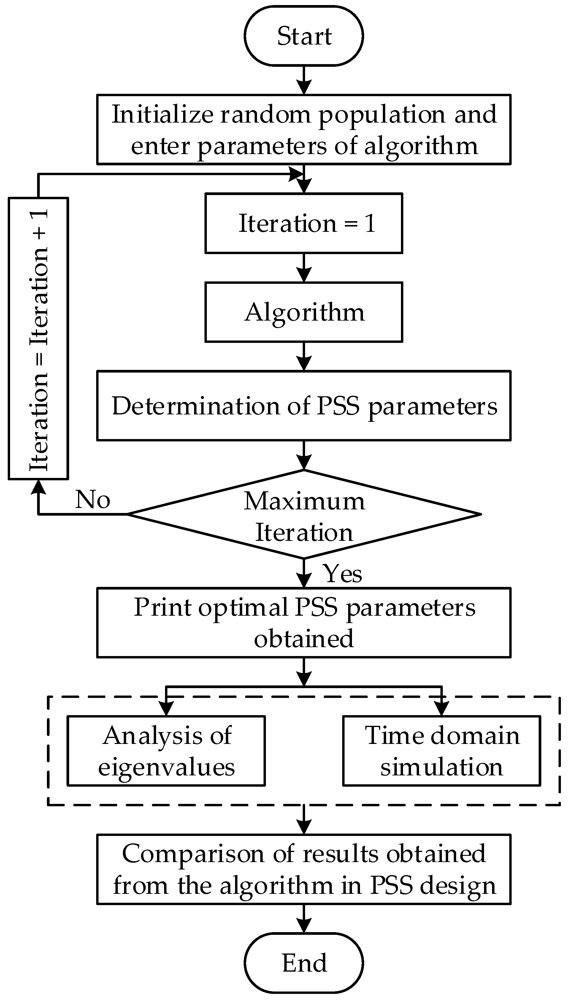
Metaheuristic algorithm techniques in PSS design have emerged recently. Several metaheuristic algorithms have been proposed for PSS design in a multi-machine power system, including the farmland fertility algorithm in [21,22], the kidney-inspired algorithm in [23], particle swarm optimization in [24,25], improved particle swarm optimization in [26,27], bacterial foraging in [28], an improved salp swarm algorithm in [29], evolutionary programming in [30], an improved Harris Hawk algorithm in [31], chaotic teaching-learning in [32], firefly algorithm in [33], cuckoo search algorithm in [34,35], new chaotic sunflower optimization in [36], whale and improved whale optimization in [37,38], gray wolf and sine-cosine were combined in [39], and ant-lion algorithm in [40]. The important advantage of metaheuristic algorithms is that their search engine simulates two important steps: exploration and exploitation. The former is concerned with locating new positions in search spaces that are distinct from the current positions in the entire search space. The former entails searching for optimally close positions. Simulating exploration only may result in new positions with low precision. On the contrary, deploying exploitation only enhances the rate of getting stuck in the local optimum positions. Hence, many new metaheuristic algorithms tend to balance the exploration and exploitation processes in their search algorithms. Metaheuristic algorithms are being developed and proposed for PSS optimization problems because of the no-free-launch theorem, which expresses that no algorithm is best for all optimization problems [1]. This study performs a comparative study of five metaheuristic algorithms: GBO and RUN, which are based on mathematical concepts, and AVOA, AEO, and GTO, which are nature-inspired for optimal PSS design in a multi-machine power system considering different operating conditions; the whole procedure is graphically represented in Figure 1. The aim is to propose the best-performing algorithms from this study.

The rest of the paper is arranged as follows: Section 2 briefly explains the mathematical modeling of the five algorithms, Section 3 describes the power system test model and PSS design, Section 4 presents the results and discussions from the analysis, and Section 5 concludes the paper.

2. Metaheuristic Algorithms

2.1. Artificial Eco-System (AEO)

The artificial ecosystem is a nature-inspired novel metaheuristic algorithm developed by [41]. The algorithm imitates the flow of energy between the three unique components in an ecosystem and their behavioral process, which are the producer (production), the consumer (consumption), and the decomposer (decomposition). The interaction between these three components makes up an ecosystem food chain, which describes the feeding process in an ecosystem and shows the flow of energy in an ecosystem. Only one producer and one decomposer exist as individuals in the ecosystem’s population. The rest of the population, representing the search space, are consumers chosen as carnivores, herbivores, or omnivores with the same probability. The defined objective function indicates an individual with a higher energy level for a minimization problem.

2.1.1. Production Process

The production process allows AEO to randomly produce a new search entity. The newly created search entity replaces the previous “best entity” (solution) $(x_n)$. This displacement is between the best entity and a new search entity randomly produced in the search space $(x_{rand})$. An operator known as a production operator is used to mathematically describe this behavior as shown in Equations (1)–(3):

$$x_1(t+1)=(1-a)x_n(t)+a{x}_{rand}(t)$$

(1)

$$a=(1-\frac{t}{maxit})r_1$$

(2)

$$x_{rand}=r\times (V_{PSS}^{max}-V_{PSS}^{min})+V_{PSS}^{min}$$

(3)

where the population size is represented by $n$, $a$ is the weight coefficient, $t$ is the current iteration, the maximum number of iterations performed or stop criteria is given as $maxit$, $V_{PSS}^{max}$ and $V_{PSS}^{min}$ are the upper PSS and lower PSS limits, respectively, and $r_1$ is a value randomly generated in the range of $\left[0, 1\right].r$ is a vector produced randomly within the range of $\left[0, 1\right].$ $x_{rand}$ is an individual position generated randomly in the search space.

2.1.2. Consumption Process

After the production process, consumption takes place among the consumers. Each consumer wishing to obtain food energy may either feed on another consumer randomly chosen with a lower energy level, a producer, or both. A consumption factor $c$, with levy flight characteristics, is proposed and defined in Equations (4) and (5) as a simple parameter-free random walk.

$$C=\frac{1}{2}\frac{v_1}{\left|v_2\right|}$$

(4)

$$v_1\in N (0, 1), v_2\in N(0, 1)$$

(5)

$v_1 \mathrm{and} v_2$ are the levy flight distributions where the normal distribution is given as $N(0, 1)$ with a standard deviation of 1 and mean of 0.

The consumption factor is crucial because it assists each consumer in hunting for food. The three consumers, carnivores, herbivores, and omnivores, adopt unique consumption strategies.

If herbivore is randomly selected as a consumer, they can only eat the producer. Its behavior is represented in a mathematical model as shown in Equation (6).

$$x_i(t+1)=x_i(t)+C\times (x_i(t)-x_1(t)), i\in \left[2,\dots ,n\right]$$

(6)

However, if a randomly chosen consumer is an omnivore, it can only eat a randomly chosen consumer with more energy. This can be shown mathematically in Equations (7) and (8):

$$x_i(t+1)=x_i(t)+C\times (x_i(t)-x_j(t)), i\in \left[3,\dots ,n\right]$$

(7)

$$j=randi(\left[2i-1\right])$$

(8)

Moreover, if an omnivore is randomly selected as a consumer, it can eat a random consumer with a higher energy level and a producer as well. It is mathematically modeled in Equations (9) and (10):

$$x_i(t+1)=x_i(t)+C\times (r_2\times (x_i(t)-x_1(t))+(1-r_2)(x_i(t)-x_j(t)),i=3,\dots ,n$$

(9)

$$j=randi(\left[2i-1\right])$$

(10)

where $r_2$ is a number generated randomly in the range of $\left[0, 1\right].$

2.1.3. Decomposition Process

The decomposition process is essential because it provides the producer with the required nutrients for growth. The decomposer chemically breaks down the remains of each individual in the population after death. Its behavior is mathematically modeled as a decomposition factor $D$ with weighting coefficients $e$ and $h$ in Equations (11)–(14) as follows:

$$x_i(t+1)=x_n(t)+D\times (e\times x_n(t)-h.x_i(t)), i=1,\dots ,n$$

(11)

$$D=3u, u\in N(0,1).$$

(12)

$$e=r_3\times randi(\left[1, 2\right])-1$$

(13)

$$h=2\times r_3-1$$

(14)

2.2. African Vulture Optimization Algorithm (AVOA)

The AVOA is like most metaheuristic algorithms that mimic the biological principles of living things. The AVOA is based on the theories and principles of Old World African vultures described in [42], with habitats in Africa, Europe, and Asia. The AVOA optimization steps are grouped into four and are presented as follows:

Step One: (Population Initialization) To determine the population where the best vulture is located, the population size is initiated, and the fitness of all members is calculated, the best solution is chosen as the best vulture of the first group; likewise, the second-best solution is the best vulture in the second group; concurrently, other solutions follow from Equation (15)

$$R(i)=\{\begin{array}{c}BestVultur{e}_{1 }if P_i=L_1\\ BestVultur{e}_2 if P_i=L_2\end{array}$$

(15)

where $L_1$ and $L_2$ are measured parameters before the search operation. They are within the range $\left[0, 1\right]$ and the sum of the two parameters is $1$. Roulette wheel selection is used for the probability of choosing the best solution from each group and is expressed in Equation (16) as

$$P_i=\frac{F_i}{{{\displaystyle \sum }}_{i=1}^n{F}_i}$$

(16)

where $F$ denotes the satisfaction rate and $P_i$ is the best solution for each group. If an $\alpha —\mathrm{numeric}$ parameter is near $1$ and the $\beta —\mathrm{numeric}$ parameter is near $0$, it increases intensification, while if the $\beta —\mathrm{numeric}$ parameter is near $1$ and the $\alpha —\mathrm{numeric}$ parameter is near $0$, it increases AVOA diversity.

Step Two: (Vulture starvation rate) The starvation rate of vultures determines the distance vultures travel in search of food (search space) Equation (17) explains this behavior.

$$t=h\times (si{n}^W(\frac{\pi }{2}\times \frac{iteratio{n}_i}{maxiterations})+cos(\frac{\pi }{2}\times \frac{iteratio{n}_i}{maxiterations}))$$

(17)

$$F=(2\times randi+1)\times z\times (1-\frac{iteratio{n}_i}{maxiterations})+1$$

(18)

where $F$ denotes satisfaction rate, $maxiterations$ represents the total number of iterations initiated, $iteratio{n}_i$ indicates the current iteration number, $z$ is a randomly generated number between $\left[-2, 2\right],randi$ value is $\left[0, 1\right]$; a value below $0$ for $z$ means the vulture is starving, while a value above or equal to $0$ means the vulture is satisfied.

Step Three: (Exploration) Vultures in the AVOA experience difficulty finding food; hence, they explore their habitat for a long time and travel far and wide in search of food. Two strategies are adopted in this search process and a parameter $P_1$ is used to decide on each strategy to be chosen. This parameter is set before the optimization operation and is within the range of $\left[0, 1\right]$.

In choosing a strategy in the exploration phase, a random number $ran{d}_{P1 }$ is generated if $ran{d}_{P1}\ge P_{1 }$ Equation (22) is used; otherwise, Equation (21) is adopted. In this scenario, each vulture randomly searches the environment for food. This behavior is modeled in Equation (19)

$$P(i+1)=\{\begin{array}{c}Equation(22) if P_1\ge ran{d}_{P1}\\ Equation(21) if P_1<ran{d}_{P1}\end{array}$$

(19)

$$P(i+1)=R(i)-F+ran{d}_2\times ((ub-lb)\times ran{d}_3+lb)$$

(20)

$$P(i+1)=R(i)-D(i)\times F$$

(21)

$$D(i)=\left|X\right|+R(i)-P(i)$$

(22)

In Equation (21), vultures initiate a random search for food in their immediate environment. The distance of the search is randomly selected for one of the best vultures of the two groups. The vulture position vector in the next iteration is expressed as $P(i+1)$, and the satisfaction rate of the vulture is $F$ computed using Equation (18) in the present iteration. $R(i)$ in Equation (21) is one of the best vultures chosen via Equation (15). $ran{d}_2$ is a random number within the range $\left[0, 1\right]$. and is used to ensure a random high coefficient at the environmental search scale; thus, increasing the variety of search space areas. $D(i)$ Equation (22) denotes the distance between the vulture and a present optimal one. $X$ is a randomly generated value within range $\left[0, 2\right]$. $ub$ and $lb$ denote the upper and lower boundary limits.

Step Four: (Exploitation) This stage is further divided into two parts.

Stage one: Stage one explores the efficiency of the AVOA. The AVOA initiates the exploitation process if $F<1$. $P_2$ is a parameter within the range $\left[0, 1\right]$ and is adopted to decide on the strategy to be selected. A strategy called siege-fight is gently applied if the value $ran{d}_{P2}\ge P_2$; otherwise, a strategy known as rotational flying is adopted. This behavior is modeled in Equation (23).

$$P(i+1)=\{\begin{array}{c}Equation(25) if P_2\ge ran{d}_{P2}\\ Equation(26) if P_2<ran{d}_{P2}\end{array}$$

(23)

$$P(i+1)=D(i)\times (F+ran{d}_4)-d(t)$$

(24)

$$P(i+1)=R(i)-(S_1+S_2)$$

(25)

$$d(i)=R(i)-P(i)$$

(26)

$ran{d}_4$ is a generated random value in the range $\left[0, 1\right]$ and $d(t)$ is the distance between one best vulture from one group to the other best vultures in the other group calculated using Equation (26).

$S_1$ and $S_2$ are computed using Equations (27) and (28) as expressed below.

$$S_1=R(i)\times (\frac{ran{d}_5\times P(i)}{2\pi })\times \cos (P(i))$$

(27)

$$S_2=R(i)\times (\frac{ran{d}_6\times P(i)}{2\pi })\times \sin (P(i))$$

(28)

$ran{d}_5$ and $ran{d}_6$ in Equations (27) and (28) are made up of random numbers between $\left[0, 1\right].$

Stage two: Stage two of the AVOA is employed if $F<0.5$. At the start, $ran{d}_{3 }$ is produced in the range $\left[0, 1\right]$. If parameter $P_3\ge ran{d}_3$, a strategy known as “competition for food” is initiated which attracts various vultures to the food source. The position of vultures is updated via Equation (29).

$$P(i+1)=\frac{A_1+A_2}{2}$$

(29)

Equations (30) and (31) compute $A_1, A_2$ as explained below.

$$A_1=BestVultur{e}_1(i)-\frac{BestVultur{e}_1(i)\times P(i)}{BestVultur{e}_1(i)-{(P(i))}^2}\times F$$

(30)

$$A_2=BestVultur{e}_1(i)-\frac{BestVultur{e}_2(i)\times P(i)}{BestVultur{e}_2(i)-{(P(i))}^2}\times F$$

(31)

In the second stage of AVOA exploitation, vultures gather toward the best vulture to feast on leftover food. As a result, the vulture’s position is updated using Equation (32).

$$P(i+1)=R(i)-d(t)\times F\times levy(d)$$

(32)

where $d$ is the problem’s dimension; the “levy flight” phenomenon enhances AVOA efficiency and is described as

$$LF(x)=0.001\times \frac{u\times \sigma }{{\left|v\right|}^{\frac{1}{P}}}$$

(33)

$$\sigma ={(\frac{\mathsf{\Gamma }(1+\beta )\times \sin (\frac{\pi \beta }{2})}{\mathsf{\Gamma }(1+\beta 2)\times \beta \times 2\times (\frac{\beta -1}{2})})}^{\frac{1}{P}}$$

(34)

$\beta =1.5 (\mathrm{Constant} \mathrm{value})$ while $v \mathrm{and} u$ are randomly generated numbers within a range of $\left[0, 1\right]$.

For more details about the AVOA, see [42].

2.3. Gorilla Troop Optimization (GTO)

A new metaheuristic algorithm inspired by the gorilla’s pack behavior and developed by [43] is mathematically modeled to explain the two important phases in optimization (exploration and exploitation). GTO algorithm uses five different operators in exploration and exploitation for optimization problems.

Exploitation: Follow the silverback; competition for adult females

Exploration: Migrate to unknown places, migrate around known places, and move to other gorilla groups.

2.3.1. Exploration Process

The process applied to the exploration phase is explained here. Gorillas live in groups under the leadership and dominance of the silverback; however, there are times when gorillas move away from their group. This movement can occur in three ways, each represented by a parameter $P$ with the range $\left[0, 1\right]$, gorillas can move to unknown places (i.e., $rand<P$), to known places (i.e., $rand\ge 0.5$), and to other gorilla groups (i.e., $rand\ge 0.5$). The first movement type provides a possibility for the algorithm to survey the entire search space well, the second movement type improves the algorithm’s exploration performance, and the third movement type enhances the algorithm’s ability to escape the local optima trap. Equation (35) models this behavior.

$$GX(t+1)=\{\begin{array}{cc}(UB-LB)\times r_1+LB& rand<P\\ (r_2-C)\times X_r(t)+L\times H& rand\ge 0.5\\ X(i)-L(L\times (X(t)-G{X}_r(t))+r_3\times (X(t)-G{X}_r(t)))& rand<0.5\end{array}$$

(35)

$GX(t+1)$ is the candidate position vector of a gorilla in the next iteration $t$. $X(t)$ is the present vector of the position of the gorilla. $r_1,r_2,r_3$, and $rand$ are random values within range $\left[0, 1\right]$ updated in each iteration. $UB$ and $LB$ denote the upper and lower limit boundaries of variables. $X_r$ is one member of the gorillas in a group that is randomly selected from the entire population and $G{X}_r$ is one of the vectors of the gorilla’s positions of the randomly selected candidate’ it also includes the updated positions in each phase. $c,$ $H$, and $L$ are computed using Equations (36)–(38).

$$C=F\times (1-\frac{It}{maxIt})$$

(36)

$$F=Cos(2\times r_4)+1$$

(37)

$$L=C\times l$$

(38)

$It$ in Equation (36) represents the iteration current value, $maxIt$ is the total number of iterations performed, $Cos$ in Equation (37) denotes the cosine function, and $r_4$ is random values within range $\left[0, 1\right]$ updated in each iteration. $l$ in Equation (38) is a random value in the range $\left[-1, 1\right]$. The silverback dominance is modeled using Equation (38). From Equation (35), $H$ is computed using Equation (39), while $Z$ is computed in Equation (40).

$$H=Z\times X(t)$$

(39)

$$Z=\left[-C, C\right]$$

(40)

where $Z$ is a random value in the dimensions of the problem within the range $\left[-C, C\right]$

2.3.2. Exploitation Process

The two behaviors applied here are following the silverback and competition for adult females. The silverback dominates the group, makes decisions for the group, directs gorillas to food sources, and determines their movements. Silverbacks may get old and die eventually, thus letting blackbacks (the young male gorillas) become the leader, or the other male gorillas may fight the silverback and dominate the group. Each of the behaviors in the exploitation phase, as already mentioned, can be selected using $C$ in Equation (36); if $C\ge W$, the following silverback behavior is selected, while if $C<W$, competition for adult females is selected. $W$ is a value to be set before optimization.

Equation (41) simulates following the silverback.

$$GX(t+1)=L\times M\times (X(t)-X_{silverback})+X_{(t)}$$

(41)

where $X_{silverback}$ is the position vector of the silverback gorilla, $X_{(t)}$ is the position vector of the gorilla, $L$ is computed using Equation (38) and $M$ is computed using Equation (42):

$$M={({\left|\frac{1}{N}{\displaystyle \sum }_{i=1}^{N}G{X}_i(t)\right|}^g)}^{\raisebox{1ex}{$1$}\!\left/ \!\raisebox{-1ex}{$g$}\right.}$$

(42)

$$g=2^L$$

(43)

where $G{X}_i(t)$ indicates each candidate gorilla’s vector position in iteration $t$, $N$ is the total gorilla numbers, $g$ is estimated via Equation (43), and $L$ in Equation (43) is computed using Equation (38):

$$Q=2\times r_5-1$$

(44)

$$A=\beta \times E$$

(45)

where $r_5$ is a random value within $\left[0, 1\right]$ range, $A$ in Equation (45) is a coefficient vector that determines the degree of violence in conflicts, $\beta$ is a parameter that is set before optimization operation, and $E$ in Equation (45) is a parameter set while being used to model the effect of violence on the dimensions of the solution. If $rand\ge 0.5$, $E_s^{\prime }$ value of $E$ is equal to random values in a normal distribution with problems dimensions, while if $rand<0.5,$ $E$ will be equal to a random value in a normal distribution. For more details about GTO see [43].

2.4. Gradient-Based Optimization (GBO)

A search engine based on newton’s method and developed by [44] employs a set of vectors to search the solution space, which involves two operators: the gradient search rule (GSR) and the local escaping operator (LEO). These two operators help balance the exploitation and exploration process.

2.4.1. Initialization

In GBO, the following vector $N$ in dimensional space $D$ describes the population and iteration numbers as shown in Equation (46).

$$X_n=X_{min}+rand(0,1)\times (X_{max}-X_{min})$$

(46)

$X_{min}$ and $X_{max}$ are the boundary limits of $X$ variables and $rand$ is a randomly generated number within range $\left[0, 1\right].$

2.4.2. GSR Process

An important factor $\rho$ is adopted in balancing the exploration of important regions in search space while maintaining near global and optimal points. The factor $\rho$ is based on the sine function and expressed as follows:

$${\rho }_1=2\times rand\times \alpha -\alpha$$

(47)

$$\alpha =\left|\beta \times \sin (\frac{3\pi }{2})+\sin (\beta \times \frac{3\pi }{2})\right|$$

(48)

$$\beta ={\beta }_{min}+({\beta }_{max}-{\beta }_{min})\times {(1-{(\frac{m}{M})}^3)}^2$$

(49)

${\beta }_{max}$ and ${\beta }_{min}$ are constant values of $0.2$ and $1.2$, respectively, the current iteration is denoted by $m$, $M$ is the maximum number of iterations, and the $\rho$ value changes during iterations of optimization. Starting with a large value to ensure wide variety, the $\rho$ value increases through defined iterations within an assigned range. Thus, increasing GBO solution diversity and providing multiple solution exploration to the problem for the algorithm. GSR is expressed as

$$GSR=randn\times {\rho }_1\times \frac{2\mathsf{\Delta }x\times x_n}{x_{worst}-x_{best}+\epsilon }$$

(50)

GBO uses a behavior that is random to create an exploration method. This includes finding local optima. From Equation (50), the random offset is specified as it deals with the difference between a randomly chosen solution $x_{r1}^m$ and the best solution $x_{best}$. $\mathsf{\Delta }x$ variable’s meaning is changed during iterations following Equation (53) below. $randn$ is an additional random number for exploration as shown below:

$$\mathsf{\Delta }x=rand(1:N)\times \left|step\right|$$

(51)

$$step=\frac{(x_{best}-x_{r1}^m)+\delta }{2}$$

(52)

$$\delta =2\times rand\times (\left|\frac{x_{r1}^m+x_{r2}^m+x_{r3}^m+x_{r4}^m}{4}-x_n^m\right|)$$

(53)

$rand(1:N)$ denotes random vector $N$ elements in range within $\left[0, 1\right],$ the integers $r_1,r_2,r_3$, and $r_{4 }$ are randomly chosen in a way that $(r_1\ne r_2\ne r_3\ne r_4\ne n$) Equation (52) expresses a step-in phase scale computed by $x_{best}$ and $x_{r1}^m$.

For convergence, movement with direction is adopted to enable convergence across the solution field $x_n$. To provide a convenient local search ability with an effect on GBO convergence, a property $DM$ uses its best vector from a population of vector candidates and sends the present vector $x_n$ in the best vector $x_{best}-x_n$ direction and is calculated as follows:

$$DM=rand\times {\rho }_2\times (x_{best}-x_n)$$

(54)

$rand$ is a uniformly generated number within range $\left[0, 1\right] \mathrm{and} {\rho }_2$ is a random value adopted to address the size phase in each vector; ${\rho }_2$ also is considered an important parameter and is calculated as

$${\rho }_2=2\times rand\times \alpha -\alpha$$

(55)

GSR and DM using Equations (56) and (57) shown below are improved based on the present vector position $x_n^m$.

$$X{1}_n^m=x_n^m-GSR+DM$$

(56)

$X{1}_n^m$ is an improved vector as a result of improved $X{1}_n^m$. From Equations (34) and (39), $X{1}_n^m$ transformation is expressed as

$$X{1}_n^m=x_n^m-randn\times {\rho }_1\times \frac{2\mathsf{\Delta }x\times x_n^m}{y{p}_n^m-y{q}_n^m+\epsilon }+randn\times {\rho }_2\times (x_{best}-x_n^m)$$

(57)

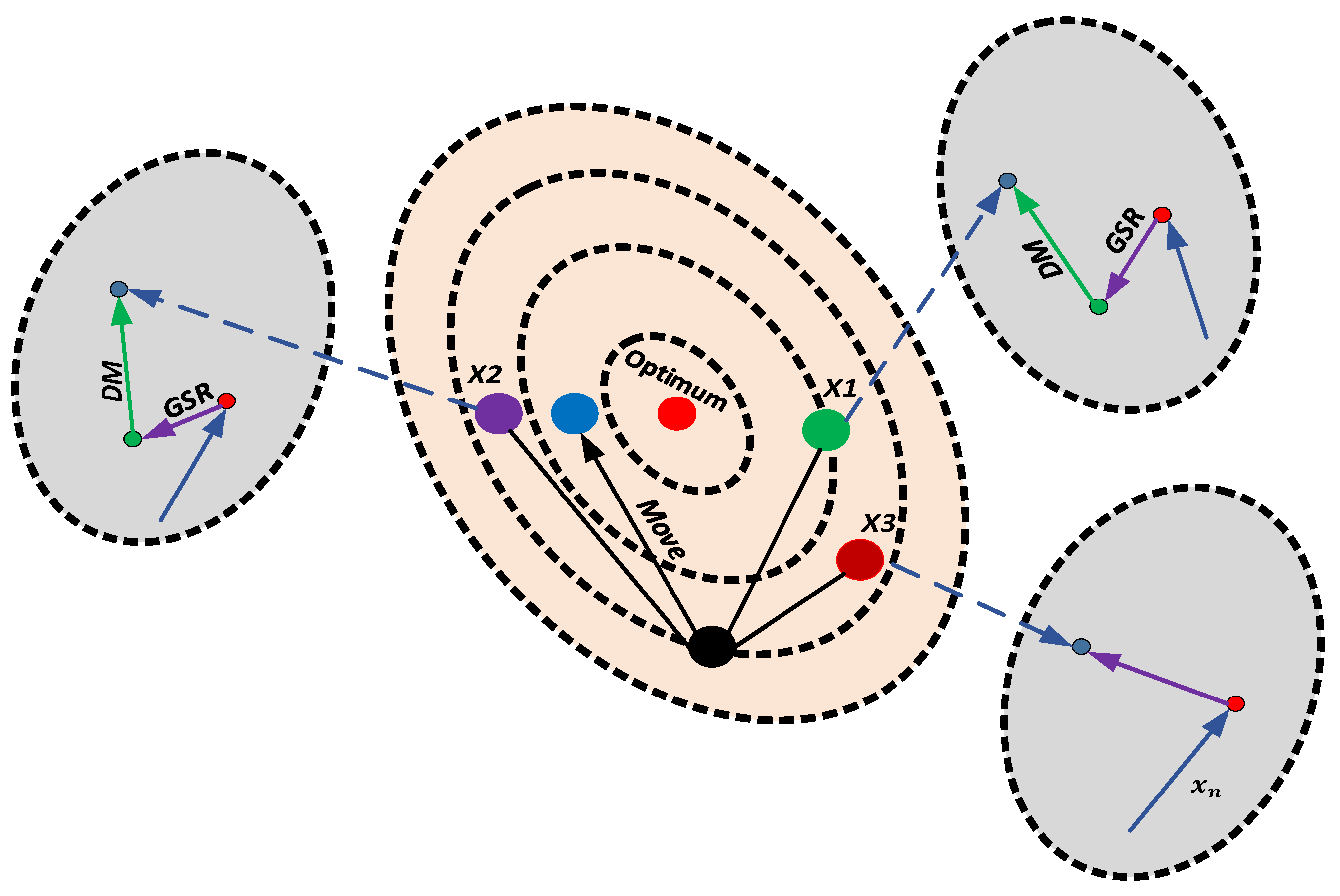
$y{p}_n^m=y_n+\mathsf{\Delta }x, y{q}_n^m=y_n-\mathsf{\Delta }x,y_n=$ average of two vectors which are the present solution $x_n \mathrm{and} z_n+1 .$ For more details about GBO see [44], Figure 2 shows the optimization process of GBO.

2.5. Runge Kutta Optimization (RUN)

The RUN algorithm concept is from the Runge-Kutta method of solving ordinary differential equations in the numeric form developed by [45]. This algorithm has two stages; the first stage procedure is based on the Runge-Kutta theory, while the second stage is known as enhanced solution quality (ESQ). The RUN algorithm is explained as follows:

Solution Updating: RUN optimization adopts a search mechanism (SM) from the Runge-Kutta concept in updating the present solution position of each iteration; this is scripted in stage one below.

Stage One: Search mechanism for updating the present solution position in RUN.

Step 1: If $rand<0.5$ then

Exploration process;

$$x_{n+1}=(X_c+r\times SF\times g\times x_c)+SF\times SM+\mu \times (randn\times (x_m-x_c))$$

(58)

Else

Exploration process;

$$x_{n+1}=(X_m+r\times SF\times g\times x_m)+SF\times SM+\mu \times (randn\times (x_{r1}-x_{r2}))$$

(59)

End if.

$r$ represents an integer number within range $\left[-1, 1\right]$ and this parameter helps in enhancing RUN diversity. $g$ is a randomly generated value within the range $\left[0, 2\right],$ as is parameter $\mu$. $SM$ is computed as in the study [30]. $SF$ is an adaptive factor computed as

$$SF=2\times (0.5-rand)\times f$$

(60)

$$F=\alpha \times \exp (-b\times rand\times (\frac{i}{maxit}))$$

(61)

$maxit$ is the maximum number of iterations and the parameters $x_m$ and $x_c$ are computed as

$$x_c=\varnothing \times x_n+(1-\varnothing )\times x_{r1}$$

(62)

$$x_m=\varnothing \times x_{best}+(1-\varnothing )\times x_{cbest}$$

(63)

$\varnothing$ is a randomly generated number within range $\left[0, 1\right]$; $x_{best}$ is the best solution found. $x_{cbest}$ is the position of the best solution found after each iteration.

Stage two: Enhanced solution quality (ESQ).

This process is adopted to increase solution quality and evade local optimal trapping during iterations. The process is scripted below:

Step 2: ESQ adoption in RUN to compute solution $x_{new2}$.

If $rand<0.5$ then

If $w<1$, then

$$x_{new2}=x_{new1}+r\times w\times \left|(x_{new1}-x_{arg})+randn\right|$$

(64)

Else

$$x_{new2}=(x_{new1}-x_{avg})+r\times w\times \left|(u.x_{new1}-x_{avg})+randn\right|$$

(65)

End if

End if.

From Step 2, $w, x_{avg}$ and $x_{new}$ new values are calculated via the below equations:

$$w=rand(0,2).\exp (-c(\frac{i}{maxit}))$$

(66)

$$x_{avg}=\frac{x_{r1}+x_{r2}+x_{r3}}{3}$$

(67)

$$x_{new1}=\beta \times x_{avg}+(1-\beta )\times x_{best}$$

(68)

$\beta$ is a randomly generated number within range $\left[0, 1\right], c=5\times rand$, the parameter $rand$ is random, and $r$ is an integer number with values $-1, 0, \mathrm{or} 1$. $x_{best}$ is the best solution found. The calculated solution $x_{new2}$ does not in each case have better fitness than the best solution. Thus, the RUN algorithm further computes $x_{new3 }$ to improve fitness via Step 3.

Step 3: Improving the new solution $x_{new3}$.

If $rand<w$, then

$$x_{new3}=(x_{new2}-rand{x}_{new2})+SF\times (ran{d}_{xRk}+(v.x_b-x_{new2}))$$

(69)

End If.

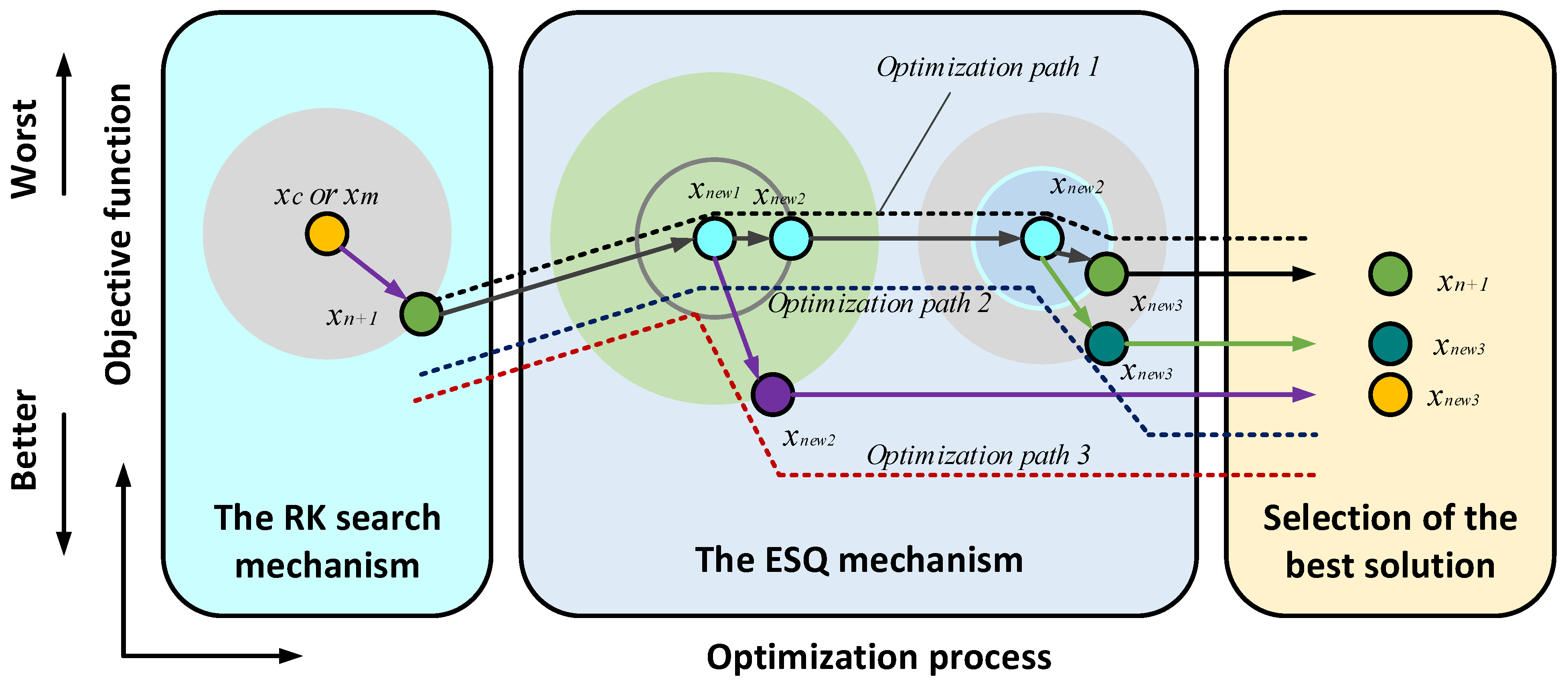
$v$ is a random number which is $2 \mathrm{rand}$. Figure 3 shows the Runge-Kutta optimization process. For more details about RUN, see [45].

3. Problem Formulation

3.1. Power System Model

The power system dynamic model is described using differential algebraic equations (DAEs) in [46] and is used to represent a power system with m-number of synchronous machines and the voltage regulator called automatic voltage regulator (AVR). The DAEs are as described in Equations (70)–(74):

$$T_{d0i}^{\prime }\frac{d{E}_{qi}^{\prime }}{dt}=-E_{qi}^{\prime }-(X_{di}-X_{di}^{\prime })I_{di}+E_{fdi}$$

(70)

$$T_{q0i}^{\prime }\frac{d{E}_{di}^{\prime }}{dt}=-E_{di}^{\prime }-(X_{qi}-X_{qi}^{\prime })$$

(71)

$$\frac{d{\delta }_i}{dt}={\omega }_i-{\omega }_s$$

(72)

$$\frac{2H_i}{{\omega }_s}\frac{d{\omega }_i}{dt}=T_{Mi}-E_{di}^{\prime }{I}_{di}-E_{qi}^{\prime }{I}_{qi}-(X_{di}-X_{di}^{\prime })I_{di}{I}_{qi}-{\mathrm{D}}_{\mathrm{i}}({\omega }_i-{\omega }_s)$$

(73)

$$T_{Ai}\frac{d{E}_{fdi}}{dt}=-K_{Ai}{E}_{fdi}+K_{Ai}(V_{refi}-V_i)$$

(74)

where in Equations (70)–(74), subscript $i$ denotes $i\mathrm{th}$ synchronous generator, $T_{d0}^{\prime }$ and $T_{q0}^{\prime }$ are the d-axis and q-axis open-circuit time constants, $E_d^{\prime }$ and $E_q^{\prime }$ are the transient EMF of the d-axis and q-axis due to flux linkage in the damper coils, $E_{fd}$ the excitation field voltage, $X_d$ and $X_q$ are the synchronous transient and sub-transient of d-axis and q-axis reactances, $\delta$ is the rotor angle of the generator, $\omega$ is the generator rotor speed, ${\omega }_s$ generator synchronous speed, $H$ is the generator inertia constant, $D$ is the damping coefficient, $T_M$ is the mechanical torque or power output, $I_d$ and $I_q$ are stator current d-axis and q-axis components, $V_{ref}$ is the reference excitation voltage, $V$ is the terminal voltage of the generator, $K_A$ is excitation static gain, $T_A$ is the regulator time constant, $T_E$ is the electrical torque, $V_d$ and $V_q$ are generator terminal voltage of the d-axis and q-axis components, and $R_s$ is the armature resistance.

$T_{Mi}$, the input mechanical torque, is kept constant in designing the excitation controller, i.e., to not significantly affect machine dynamics, the generator action is assumed to be slow. Electrical torque is substituted in Equation (73) as follows:

$$T_{Ei}=E_{di}^{\prime }{I}_{di}+E_{di}^{\prime }{I}_{di}+(X_{qi}^{\prime }-X_{di}^{\prime })I_{di}{I}_{qi}$$

(75)

A power grid system of n number of buses and m number of generators, with load buses m-n described using algebraic equations as follows from Equations (76)–(78):

$$\begin{gathered} 0=V_i{e}^{j\theta i}+(R_{si}+j{X}_{di}^{\prime })(I_{di}+j{I}_{qi})e^{j(\delta i-\frac{\pi }{2})}-\left[E_{di}^{\prime }+(X_{qi}^{\prime }-X_{di}^{\prime })I_{qi}+j{E}_{qi}^{\prime }\right]e^{j(\delta i-\frac{\pi }{2})} \\ i=1,\dots ,m \end{gathered}$$

(76)

$$V_i{e}^{j\theta i}(I_{di}+j{I}_{qi})+P_{Li}(V_i)+j{Q}_{Li}(V_i)={\displaystyle \sum }_{k=1}^n{V}_i{V}_k{Y}_{ik}{e}^{j(\theta i-\theta k-{\alpha }_{ik})},i=1,\dots ,m$$

(77)

$$P_{Li}(V_i)+j{Q}_{Li}(V_i)={\displaystyle \sum }_{k=1}^n{V}_i{V}_k{Y}_{ik}{e}^{j(\theta i-\theta k-{\alpha }_{ik})},i=m+1,\dots ,n$$

(78)

The load active power and reactive power are represented by $P_L$ and $Q_L$, respectively. $\mathrm{Yej}\mathsf{\alpha }$ denotes the power system admittance matrix and $\theta$ is the bus voltage $V$ angle. The admittance matrix load element in power lines is reduced by the order reduction method, as in Equation (79).

$$\mathsf{\Delta }\dot{x=Ax+Bu,}$$

(79)

The power system linear model is described using Equation (79), where $x$ is the system state vector variables, $A$ the state space matrix of the system, $B$ is the system input matrix, and $u$ is the system control input vector.

$$G_i(s)=\frac{V_{PSSi(s)}}{\mathsf{\Delta }{w}_i(s)}=K_{Gi}\frac{T_{w}s}{(1+s{T}_w)}\frac{(1+s{T}_{1i})}{(1+s{T}_{2i})}\frac{(1+s{T}_{3i})}{(1+s{T}_{4i})}$$

(80)

3.2. PSS Design Procedure

For analysis, this study employs a conventional lead-lag PSS connected to an IEEE-ST1-type excitation [18]. The ith system transfer function in Equation (80) describes the PSS connection with the IEEE-ST1 excitation system.

Where the output signal of the PSS at the ith machine is $V_{PSSi}$, $T_w$ is the washout time constant equal to 10 in this study, synchronous machine speed deviation signal is $\mathsf{\Delta }{w}_i$. Optimal parameters of stabilizer gain $K_{pssi}$ and parameters $T_{i1}$, $T_{i2},$ $T_{i3}$, and $T_{i4}$, are to be determined.

An eigenvalue objective function is employed to enhance the damping characteristics of electromechanical modes (EMs) of the system and shift the eigenvalues of the power system to the left region of the complex s-plane. Stabilizer gain and parameters of the PSS are determined through the defined eigenvalue objective function as follows in Equation (81):

$$\begin{gathered} J_{eig}=max\left\{real({\lambda }_i)|{\lambda }_i ϵ EMs\right\}+P_C{{\displaystyle \sum }}^{ }\left\{real({\lambda }_j)|{\lambda }_j>0\right\} \\ EMs=\left\{{\lambda }_k|0<\frac{im({\lambda }_k)}{2\pi }<5\right\} \end{gathered}$$

(81)

Eigenvalues of the power system state space matrix are denoted by ${\lambda }_i$, while $P_C$ is a penalty constant applied in producing positive eigenvalues and can enhance slow eigenvalues [18]. In this study, $P_C$ is 50. $J_{eig}$, which is the objective function, is minimized subject to PSS gain $(K_{pssi})$ and time constants ($T_{1i},T_{2i},T_{3i},$ and $T_{4i})$ constraints ($0.001\le K_{pssi}\le 50$ and $0.001\le T_{1i}\le 1$, $0.001\le T_{3i}\le 1$, 0.001, and $0.02\le T_{4i}\le 1$) [47].

4. Results and Discussion

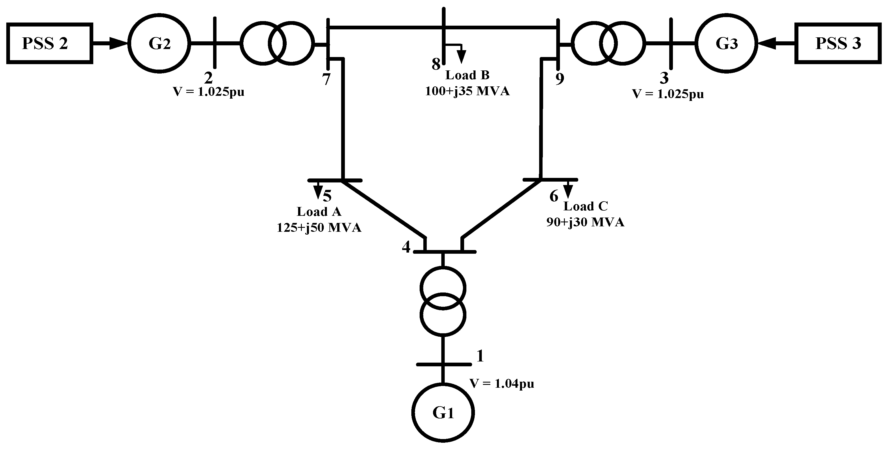
The power test system adopted in this study is the Western System Coordinating Council (WSCC), which is a three-machine, nine-bus test system, as seen in Figure 4 below. The modeling parameters for the test system are shown in

Table 1. Parameters of the WSCC test system.

Parameter	Value
Transmission line	$X_{T14}=0.0576 \mathrm{pu},X_{T27}=0.0625 \mathrm{pu},X_{T39}=0.0586 \mathrm{pu},$ $X_{T45}=0.085 \mathrm{pu},X_{T46}=0.092 \mathrm{pu},X_{T57}=0.161 \mathrm{pu},$ $X_{T69}=0.17 \mathrm{pu},X_{T78}=0.072 \mathrm{pu},X_{T89}=0.1008 \mathrm{pu},$ $X_{L14}=0 \mathrm{pu},X_{L27}=0 \mathrm{pu},X_{L39}=0 \mathrm{pu},X_{L45}=0.176 \mathrm{pu},$ $X_{L46}=0.158 \mathrm{pu},X_{L57}=0.306 \mathrm{pu},X_{L69}=0.358 \mathrm{pu},$ $X_{L78}=0.149 \mathrm{pu},X_{L89}=0.209 \mathrm{pu},$
Machine	$H_1=23.63 \mathrm{s}, H_2=6.4 \mathrm{s},H_3=3.01 \mathrm{s},D=0.0, T_{d01}^{\prime }=8.96 \mathrm{s},$ $T_{d02}^{\prime }=6.0 \mathrm{s},T_{d03}^{\prime }=5.89 \mathrm{s}, T_{q01}^{\prime }=0.31 \mathrm{s},T_{q02}^{\prime }=0.535 \mathrm{s},$ $T_{q03}^{\prime }=0.6 \mathrm{s}, X_{q1}=0.0969,X_{q2}=0.8645,$ $X_{q3},=1.2578, X_{d1}=0.146,X_{d2}=0.8958,X_{d3}=1.3125,$ $X_{q1}^{\prime }=0.0969 \mathrm{s}, X_{q2}^{\prime }=0.8645 \mathrm{s},X_{q3}^{\prime }=1.2578 \mathrm{s},$ $X_{d1}^{\prime }=0.0608 \mathrm{s},X_{d2}^{\prime }=0.1198 \mathrm{s},X_{d3}^{\prime }=0.1813 \mathrm{s}$ $X_d=0.8958, X_q^{\prime }=0.1969 \mathrm{s}, X_d^{\prime }=0.1198 \mathrm{s}$
Exciter	$K_{A1}=20.0, T_{A1}=0.2 \mathrm{s}, K_{A2}=20.0, T_{A2}=0.2 \mathrm{s}, K_{A3}=20.0,$ $T_{A3}=0.2 \mathrm{s}$

. The standard parameters for the generators and loads can be seen in the Figure 4. PSSs are coupled to generators (G2 and G3), with a washout time constant $T_w=10$. The total number of parameters optimized was 10 (i.e., five for each PSS). The five algorithms were run 15 times on the model separately, and the parameter settings are shown in

Table 2. Parameter settings of the five algorithms in PSSs design.

Parameter	Value
Population size	$100$
Number of variables	$10(K_{pss2},K_{pss3},T_{21}{T}_{22},T_{23},T_{24},T_{31},T_{32},T_{33},T_{34})$
Maximum iteration	$100$
Lower bound	$\left[0.001,0.001,0.001,0.02,0.001,0.02,0.001,0.02,0.001,0.02\right]$
Upper bound	$\left[50,50,1,1,1,1,1,1,1,1\right]$
Number of runs	$15$
Simulation time	$5 \mathrm{s}$

. The study is carried out under different operating conditions as shown in

Table 3. Operating conditions for the WSCC test system in 100 MVA per unit used for simulation.

Generator	Base Condition		Condition 1		Condition 2		Condition 3
	P	Q	P	Q	P	Q	P	Q
G1	0.72	0.27	2.21	1.09	0.36	0.16	0.33	1.12
G2	1.63	0.07	1.92	0.56	0.80	−0.11	2.00	0.57
G3	0.85	−0.11	1.28	0.36	0.45	−0.20	1.50	0.38
Load	Base Condition		Condition 1		Condition 2		Condition 3
	P	Q	P	Q	P	Q	P	Q
A	1.25	0.50	2.00	0.80	0.65	0.55	1.50	0.90
B	0.90	0.30	1.80	0.60	0.45	0.35	1.201	0.80
C	1.00	0.35	1.50	0.60	0.50	0.25	1.00	0.50

; a 100 MVA per unit scale was used. The optimal PSS parameters obtained for generators (G2 and G3) under base condition is shown in Table 4. Five dominant modes of the power test system are considered as shown in Table 5. Then, eigenvalues and nonlinear time-domain analysis simulation were run under a 100 ms symmetrical three-phase fault observed at $t=1 \mathrm{s}$ for different operating conditions.

4.1. Base Condition

In the base operating condition from Table 3, the optimal PSS parameters obtained for generators (G2 and G3) are shown in Table 4, where the optimized PSS parameters were used to carry out a small signal stability analysis (SSA).

Table 4. Optimal PSS parameters.

	Algorithm	$K_{PSS2}$	$T_{21}$	$T_{22}$	$T_{23}$	$T_{24}$
G2	AEO	6.2789	0.5222	0.0216	0.5813	0.0315
	AVOA	6.0246	0.5609	0.0318	0.5622	0.0220
	GTO	4.5150	0.6839	0.0309	0.6122	0.0263
	RUN	3.5079	0.7349	0.0223	0.7106	0.0343
	GBO	3.9795	0.8135	0.0257	0.4994	0.0242
	Algorithm	$K_{PSS3}$	$T_{31}$	$T_{32}$	$T_{33}$	$T_{34}$
G3	AEO	6.1017	0.0018	0.1678	0.0012	0.2185
	AVOA	4.8140	0.0197	0.3420	0.1815	0.2420
	GTO	2.5359	0.0036	0.9930	0.9996	0.3233
	RUN	2.5617	0.5713	0.0202	0.5842	0.0209
	GBO	3.0922	0.8156	0.0329	0.6459	0.0287

Table 4. Optimal PSS parameters.

	Algorithm	$K_{PSS2}$	$T_{21}$	$T_{22}$	$T_{23}$	$T_{24}$
G2	AEO	6.2789	0.5222	0.0216	0.5813	0.0315
	AVOA	6.0246	0.5609	0.0318	0.5622	0.0220
	GTO	4.5150	0.6839	0.0309	0.6122	0.0263
	RUN	3.5079	0.7349	0.0223	0.7106	0.0343
	GBO	3.9795	0.8135	0.0257	0.4994	0.0242
	Algorithm	$K_{PSS3}$	$T_{31}$	$T_{32}$	$T_{33}$	$T_{34}$
G3	AEO	6.1017	0.0018	0.1678	0.0012	0.2185
	AVOA	4.8140	0.0197	0.3420	0.1815	0.2420
	GTO	2.5359	0.0036	0.9930	0.9996	0.3233
	RUN	2.5617	0.5713	0.0202	0.5842	0.0209
	GBO	3.0922	0.8156	0.0329	0.6459	0.0287

With NO-PSS on the power system, the electromechanical modes 1 and 2 $(-0.686\pm 12.776i \mathrm{and}-0.123\pm 8.287i)$ with weak damping ratios are significantly changed after the optimization process, particularly for RUN $(-4.989\pm 15.024i,-3.834\pm 8.270i)$ and GBO $(-4.875\pm 18.240i,-3.795\pm 7.660i)$ algorithms as shown in Table 5. Moreover, the worst damping ratio of 0.0148 was enhanced to 0.4203 for RUN and 0.4439 for GBO as shown in

Table 6. Eigenvalue damping ratio and frequency.

Modes	NO-PSS		AEO		AVOA		GTO		RUN		GBO
	Damping Ratio	Frequency	Damping Ratio	Frequency	Damping Ratio	Frequency	Damping Ratio	Frequency	Damping Ratio	Frequency	Damping Ratio	Frequency
1	0.0536	2.0333	0.2532	1.8072	0.2426	1.8118	0.2600	1.8190	0.3152	2.3911	0.2581	2.9037
2	0.0148	1.3189	0.2660	1.8003	0.2725	1.8010	0.2592	1.8155	0.4203	1.3170	0.4439	1.2192
3	0.6726	0.4165	0.7001	0.4796	0.6790	0.4894	0.7106	0.4876	0.7819	0.4869	0.7736	0.5069
4	0.9593	0.2188	0.9040	0.3235	0.9134	0.3147	0.8838	0.3537	0.8677	0.3494	0.8646	0.3504
5	0.9608	0.1616	0.8544	0.3266	0.9076	0.2473	0.9070	0.2662	0.8782	0.3322	0.8716	0.3392

.

Table 5. Eigenvalue results for NO-PSS and the algorithms after optimization in base operating condition.

Modes	NO-PSS	AEO	AVOA	GTO	RUN	GBO
1	$-0.686\pm 12.776i$	$-2.972\pm 11.355i$	$-2.847\pm 11.384i$	$-3.077\pm 11.429i$	$-4.989\pm 15.024i$	$-4.875\pm 18.240i$
2	$-0.123\pm 8.287i$	$-3.121\pm 11.312i$	$-3.205\pm 11.316i$	$-3.062\pm 11.407i$	$-3.834\pm 8.270i$	$-3.795\pm 7.660i$
3	$-2.379\pm 2.617i$	$-2.955\pm 3.014i$	$-2.844\pm 3.075i$	$-3.094\pm 3.064i$	$-3.837\pm 3.051i$	$-3.888\pm 3.185i$
4	$-4.671\pm 1.375i$	$-4.298\pm 2.033i$	$-4.435\pm 1.977i$	$-4.199\pm 2.222i$	$-3.832\pm 2.190i$	$-3.789\pm 2.202i$
5	$-3.5199\pm 1.016i$	$-3.374\pm 2.052i$	$-3.360\pm 1.554i$	$-3.603\pm 1.670i$	$-3.832\pm 2.090i$	$-3.789\pm 2.131i$

Table 5. Eigenvalue results for NO-PSS and the algorithms after optimization in base operating condition.

Modes	NO-PSS	AEO	AVOA	GTO	RUN	GBO
1	$-0.686\pm 12.776i$	$-2.972\pm 11.355i$	$-2.847\pm 11.384i$	$-3.077\pm 11.429i$	$-4.989\pm 15.024i$	$-4.875\pm 18.240i$
2	$-0.123\pm 8.287i$	$-3.121\pm 11.312i$	$-3.205\pm 11.316i$	$-3.062\pm 11.407i$	$-3.834\pm 8.270i$	$-3.795\pm 7.660i$
3	$-2.379\pm 2.617i$	$-2.955\pm 3.014i$	$-2.844\pm 3.075i$	$-3.094\pm 3.064i$	$-3.837\pm 3.051i$	$-3.888\pm 3.185i$
4	$-4.671\pm 1.375i$	$-4.298\pm 2.033i$	$-4.435\pm 1.977i$	$-4.199\pm 2.222i$	$-3.832\pm 2.190i$	$-3.789\pm 2.202i$
5	$-3.5199\pm 1.016i$	$-3.374\pm 2.052i$	$-3.360\pm 1.554i$	$-3.603\pm 1.670i$	$-3.832\pm 2.090i$	$-3.789\pm 2.131i$

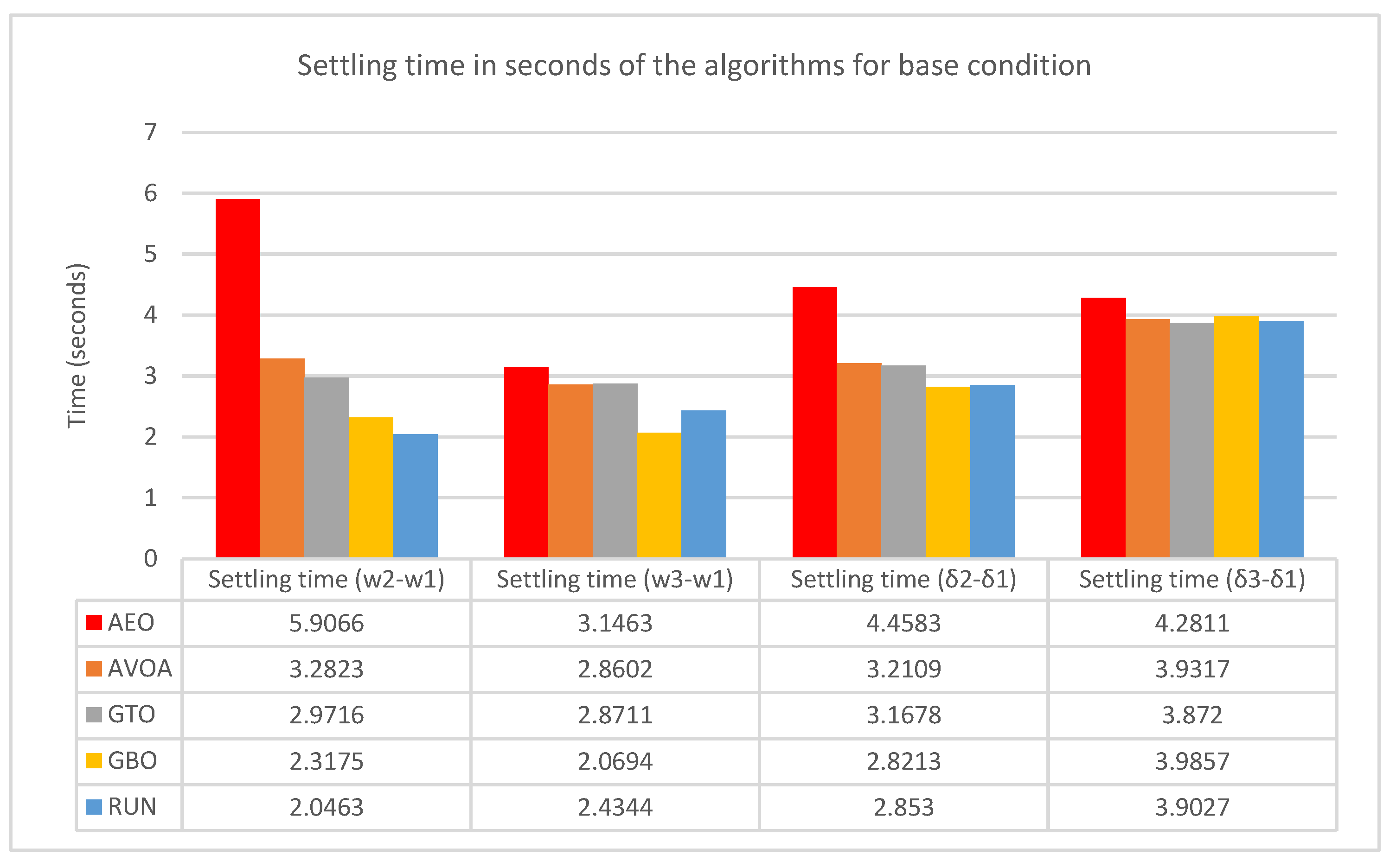
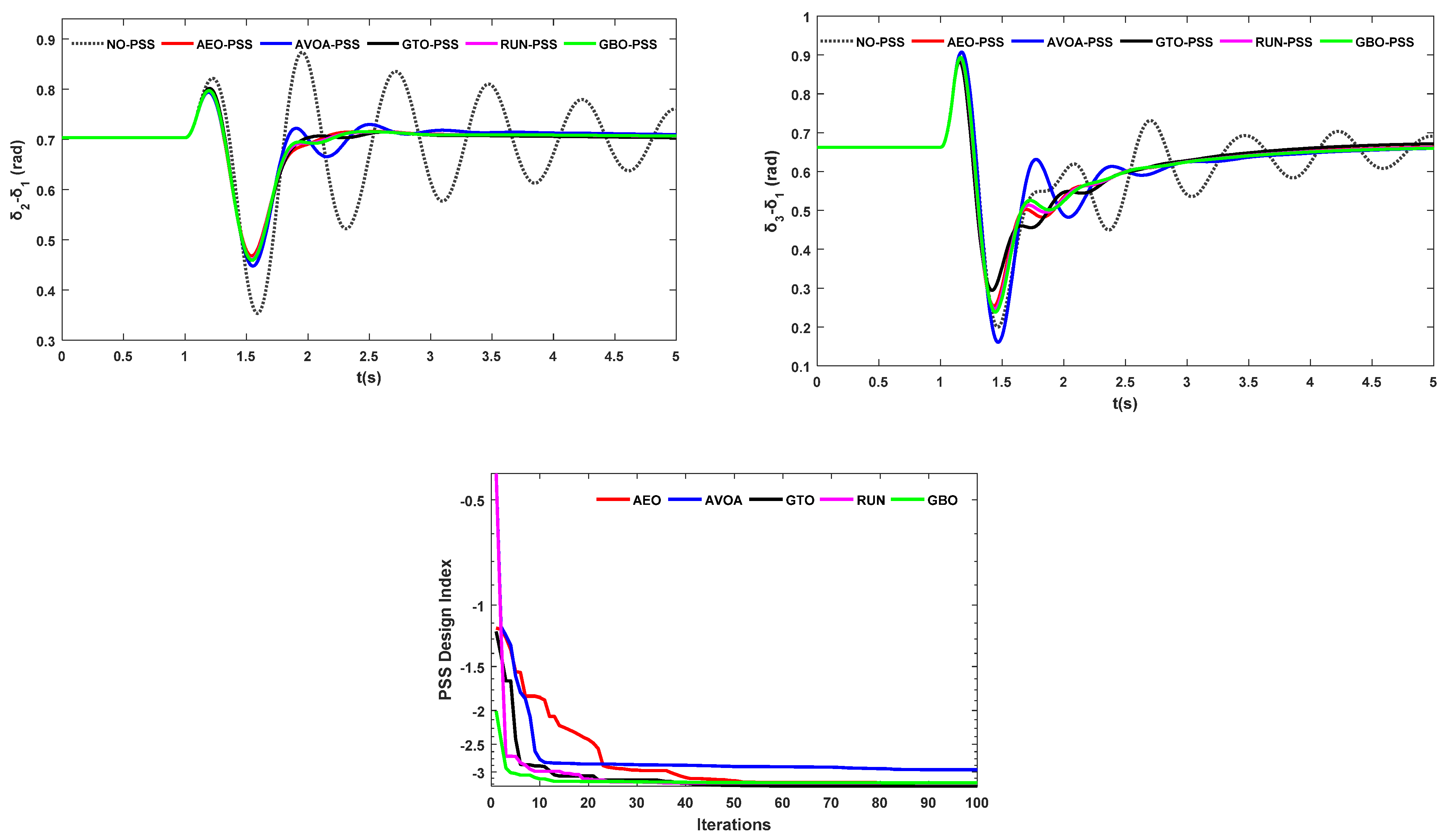
The system is restored to its original form after fault clearance, and generator rotor speed and angle variations indicate the status of stability in the power system. Hence, rotor speed deviations $({\omega }_2-{\omega }_1, {\omega }_3-{\omega }_1)$ and angle deviations of generators 2 and 3 with respect to generator 1 $({\delta }_2-{\delta }_1, {\delta }_3-{\delta }_1)$ are shown graphically in Figure 5. The time domain simulations and convergence curve results of Figure 5 show that RUN and GBO designed PSSs, which are mathematically inspired, effectively damp oscillations compared to AEO, AVOA, and GTO that are nature-inspired and hence the two algorithms are recommended for robust optimal PSSs design.

Table 7. Transient stability analysis of base condition time-domain simulations.

Algorithms	${\omega }_2-{\omega }_1$		${\omega }_3-{\omega }_1$
	Rise Time (s)	Settling Time (s)	Rise Time (s) ($\times {10}^{-4}$)	Settling Time (s)
AEO	0.00046	5.9066	1.1522	3.1463
AVOA	0.0046	3.2823	8.8800	2.8602
GTO	0.0035	2.9716	6.8550	2.8711
GBO	0.0022	2.3175	5.6230	2.0694
RUN	0.0024	2.0463	6.1301	2.4344
Algorithms	${\delta }_2-{\delta }_1$		${\delta }_3-{\delta }_1$
	Rise Time (s)	Settling Time (s)	Rise time (s) ($\times {10}^{-4}$)	Settling Time (s)
AEO	0.0016	4.4583	66.000	4.2811
AVOA	0.0154	3.2109	7.1930	3.9317
GTO	0.0149	3.1678	8.3940	3.8720
GBO	0.0135	2.8213	7.8607	3.9857
RUN	0.0132	2.8530	7.9990	3.9027

indicates transient analysis from Figure 5 in terms of rise time and settling time, which are key indicators of the performance of each algorithm. Furthermore, the settling time which is the time it takes each algorithm applied in PSS’s design to stabilize and control the low-frequency oscillation due to fault in the system has been presented in a bar chart in Figure 6. Without a PSS controller, the system is unstable for the period of simulation; hence, its settling time is not considered. For the five algorithms compared, GBO and RUN show slight improvements from the bar charts for rotor speed deviations $({\omega }_2-{\omega }_1, {\omega }_3-{\omega }_1)$ and angle deviations of generators 2 and 3 with respect to generator 1 $({\delta }_2-{\delta }_1, {\delta }_3-{\delta }_1)$.

4.2. Condition 1

To further verify the robustness of RUN and GBO-based PSSs, the operating conditions were changed from Table 3. Figure 7 graphically indicates the generator rotor speed deviations $({\omega }_2-{\omega }_1, {\omega }_3-{\omega }_1)$ and angle deviations of generators 2 and 3 with respect to generator 1, as well as the convergence curve results $({\delta }_2-{\delta }_1, {\delta }_3-{\delta }_1)$.

Table 8. Transient stability analysis of condition 1-time domain simulations.

Algorithms	${\omega }_2-{\omega }_1$		${\omega }_3-{\omega }_1$
	Rise Time (s)	Settling Time (s)	Rise Time (s)	Settling Time (s)
AEO	0.0037	2.9400	0.0016	2.9637
AVOA	0.0012	3.2454	0.00058	3.0309
GTO	0.0046	2.9307	0.0020	2.8008
GBO	0.0040	2.7993	0.0018	2.0736
RUN	0.0041	2.6255	0.0018	2.4559
Algorithms	${\delta }_2-{\delta }_1$		${\delta }_3-{\delta }_1$
	Rise Time (s)	Settling Time (s)	Rise Time (s)$(\times {10}^{-4})$	Settling Time (s)
AEO	0.000008	3.0845	0.0150	3.2810
AVOA	0.0134	3.1465	1.2119	3.2913
GTO	0.0015	3.0561	1.1691	3.2376
GBO	0.0024	2.6180	2.8990	3.1512
RUN	0.0052	2.3847	1.8165	3.3010

indicates transient analysis from Figure 7 in terms of rise time and settling time, which are key indicators of the performance of each algorithm. Furthermore, the settling time, which is the time it takes each algorithm applied in PSS’s design to stabilize and control the low-frequency oscillation due to fault in the system, has been presented in a bar chart in Figure 8. Without a PSS controller, the system is unstable for the period of simulation; hence, its settling time is not considered. For the five algorithms compared, GBO and RUN show slight improvements from the bar charts for rotor speed deviations $({\omega }_2-{\omega }_1, {\omega }_3-{\omega }_1)$ and angle deviations of generators 2 and 3 with respect to generator 1 $({\delta }_2-{\delta }_1, {\delta }_3-{\delta }_1)$.

4.3. Condition 2

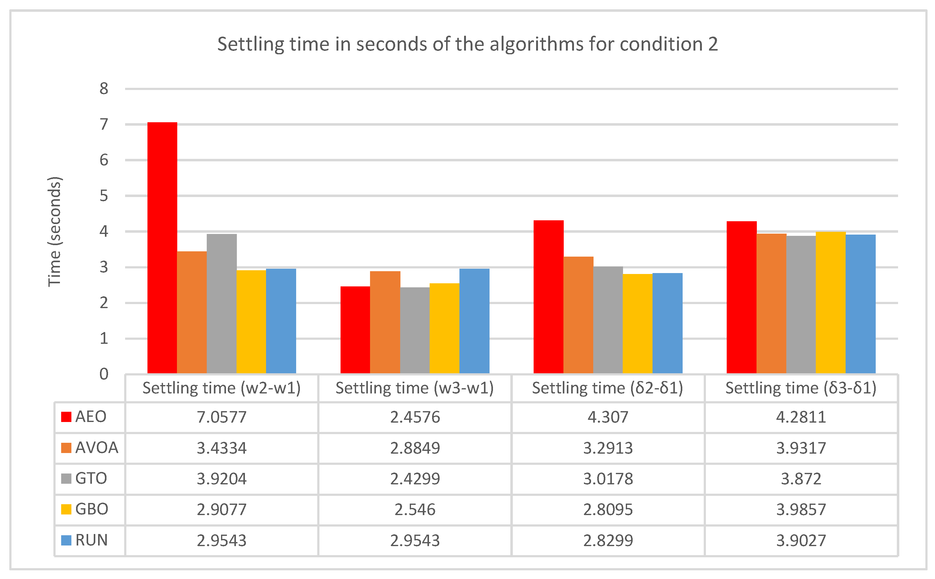
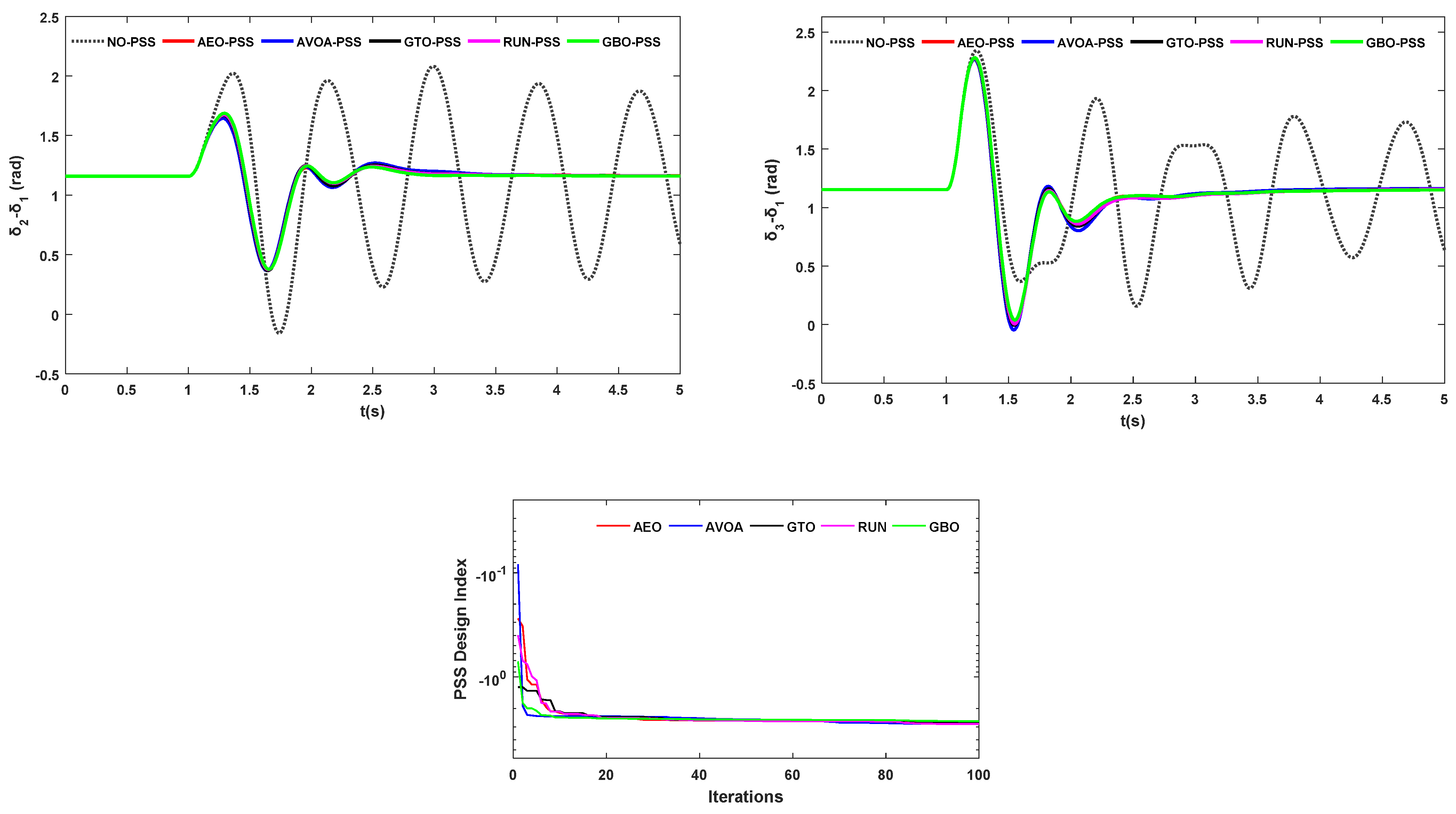
The operating conditions were again changed from Table 3. Figure 9 graphically indicates the generator rotor speed $({\omega }_2-{\omega }_1, {\omega }_3-{\omega }_1)$ and angle deviations of generators 2 and 3 with respect to generator 1, as well as the convergence curve results $({\delta }_2-{\delta }_1, {\delta }_3-{\delta }_1)$.

Table 9. Transient stability analysis of condition 2-time domain simulations.

Algorithms	${\omega }_2-{\omega }_1$		${\omega }_3-{\omega }_1$
	Rise Time (s)	Settling Time (s)	Rise Time (s)	Settling Time (s)
AEO	0.0060	7.0577	0.0011	2.4576
AVOA	0.0121	3.4334	0.0020	2.8849
GTO	0.0075	3.9204	0.0015	2.4299
GBO	0.0106	2.9077	0.0020	2.5460
RUN	0.0101	2.9543	0.0101	2.9543
Algorithms	${\delta }_2-{\delta }_1$		${\delta }_3-{\delta }_1$
	Rise Time (s)	Settling Time (s)	Rise Time (s)	Settling Time (s)
AEO	0.0028	4.3070	0.01110	4.2811
AVOA	0.0226	3.2913	0.00056	3.9317
GTO	0.0031	3.0178	0.01590	3.8720
GBO	0.0161	2.8095	0.00050	3.9857
RUN	0.0159	2.8299	0.00016	3.9027

indicates transient analysis from Figure 9 in terms of rise time and settling time, which are key indicators of the performance of each algorithm. Furthermore, the settling time, which is the time it takes each algorithm applied in PSS’s design to stabilize and control low-frequency oscillation due to faults in the system, has been presented in a bar chart in Figure 10. Without a PSS controller, the system is unstable for the period of simulation; hence, its settling time is not considered. Of the five algorithms compared, GBO and RUN show slight improvements from the bar charts for rotor speed deviations $({\omega }_2-{\omega }_1, {\omega }_3-{\omega }_1)$ and angle deviations of generators 2 and 3 with respect to generator 1 $({\delta }_2-{\delta }_1, {\delta }_3-{\delta }_1)$.

4.4. Condition 3

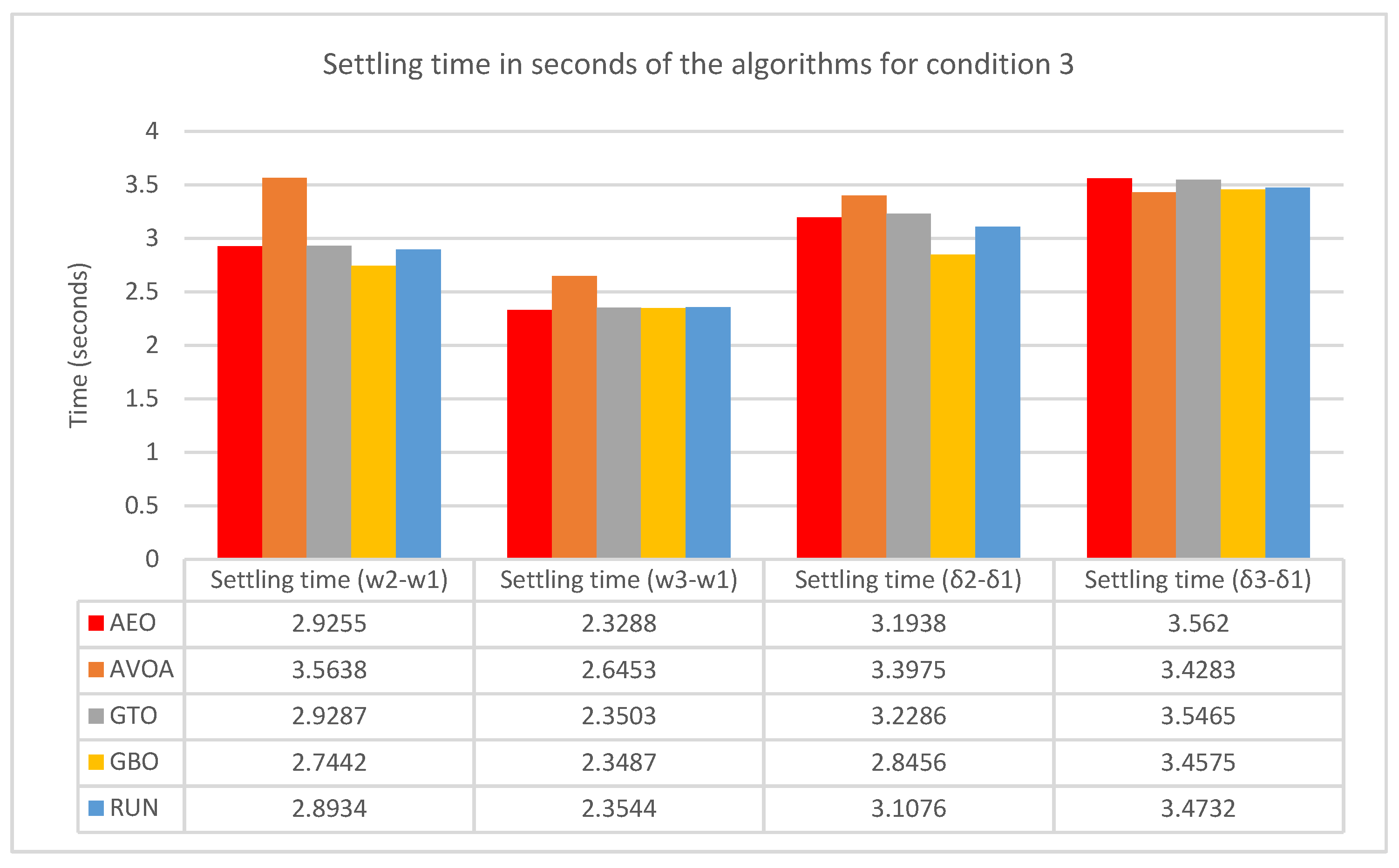
Condition 3 operating conditions are in Table 3. Figure 11 graphically indicates the generator rotor speed $({\omega }_2-{\omega }_1, {\omega }_3-{\omega }_1)$ and angle deviations of generators 2 and 3 with respect to generator 1, as well as the convergence curve results $({\delta }_2-{\delta }_1, {\delta }_3-{\delta }_1)$.

Table 10. Transient stability analysis of condition 3-time domain simulations.

Algorithms	${\omega }_2-{\omega }_1$		${\omega }_3-{\omega }_1$
	Rise Time (s) ($\times {10}^{-4}$)	Settling Time (s)	Rise Time (s) ($\times {10}^{-4}$)	Settling Time (s)
AEO	9.3990	2.9255	4.1200	2.3288
AVOA	4.5786	3.5638	1.8760	2.6453
GTO	10.000	2.9287	4.2604	2.3503
GBO	43.000	2.7442	16.000	2.3487
RUN	12.000	2.8934	4.8472	2.3544
Algorithms	${\delta }_2-{\delta }_1$		${\delta }_3-{\delta }_1$
	Rise Time (s)	Settling Time (s)	Rise Time (s)	Settling Time (s)
AEO	0.0113	3.1938	0.0026	3.5620
AVOA	0.0092	3.3975	0.0104	3.4283
GTO	0.0104	3.2286	0.0056	3.5465
GBO	0.0094	2.8456	0.00019	3.4575
RUN	0.0103	3.1076	0.0048	3.4732

indicates transient analysis from Figure 11 in terms of rise time and settling time, which are key indicators of the performance of each algorithm. Furthermore, the settling time, which is the time it takes each algorithm applied in PSS’s design to stabilize and control the low-frequency oscillation due to fault in the system, has been presented in a bar chart in Figure 12. Without a PSS controller, the system is unstable for the period of simulation; hence, its settling time is not considered. Of the five algorithms compared, GBO and RUN show slight improvements from the bar charts for rotor speed deviations $({\omega }_2-{\omega }_1, {\omega }_3-{\omega }_1)$ and angle deviations of generators 2 and 3 with respect to generator 1 $({\delta }_2-{\delta }_1, {\delta }_3-{\delta }_1)$.

5. Conclusions

This study compared five meta-heuristic optimization algorithms for PSSs design to damp low-frequency oscillation in a multi-machine power system. Three of the five algorithms are nature-inspired (AEO, AVOA, and GTO) while the remaining two are based on mathematical concepts (RUN and GBO). An eigenvalue objective function was defined to achieve this aim. Eigenvalue analysis and time domain simulations were carried out under three operating conditions in the multi-machine system. In the base condition, the optimized PSS parameters used for small signal stability analysis improved the damping ratio of the system with NO-PSS controller from 0.0148 (1.48%) to 0.2660 (26.6%) for AEO-PSS, 0.2725 (27.25%) for AVOA-PSS, 0.2592 (25.92%) for GTO-PSS, 0.4203 (42.03%) for RUN-PSS, and 0.4439 (44.39%) for GBO-PSS. Furthermore, in the time domain simulation of the different conditions (base, condition 1, 2, and 3) run for 5 s, GBO and RUN provided slight overall improvement in settling time for the generator rotor speed deviations $({\omega }_2-{\omega }_1, {\omega }_3-{\omega }_1)$ and angle deviations $({\delta }_3-{\delta }_1, {\delta }_3-{\delta }_1)$ of generators 2 and 3 with respect to generator 1. This improvement is evident in the bar graphs plot for the settling time values. The power test model used in this study was the Western System Coordinating Council power test system, which is a standard IEEE test system. It is safe to say and thus recommended that this research can be applied to a larger test system (for example, the 10-machine New England test system) and it should give the same results. Conclusively, RUN and GBO outperformed AEO, AVOA, and GTO in optimally designing lead-lag PSSs for the multi-machine power system and hence strengthens the claim made by [30] in the run beyond metaphor that most metaphor-based nature-inspired algorithms in AEO, AVOA, and GTO that imitate search patterns in animals might have limitations in an optimization problem.

References

1. Sabo, A.; Kolapo, B.Y.; Odoh, T.E.; Dyari, M.; Abdul Wahab, N.I.; Veerasamy, V. Solar, Wind and Their Hybridization Integration for Multi-Machine Power System Oscillation Controllers Optimization: A Review. Energies 2023, 16, 24. [Google Scholar] [CrossRef]
2. Sabo, A.; Abdul Wahab, N.I.; Othman, M.L.; Mohd Jaffar, M.Z.A.; Beiranvand, H. Optimal design of power system stabilizer for multimachine power system using farmland fertility algorithm. Int. Trans. Electr. Energy Syst. 2020, 30, e12657. [Google Scholar] [CrossRef]
3. Hannan, M.A.; Islam, N.N.; Mohamed, A.; Lipu, M.S.H.; Ker, P.J.; Rashid, M.M.; Shareef, H. Artificial intelligent based damping controller optimization for the multi-machine power system: A review. IEEE Access 2018, 6, 39574–39594. [Google Scholar] [CrossRef]
4. Moshtaghi, H.R.; Eshlaghy, A.T.; Motadel, M.R. A Comprehensive Review on Meta-Heuristic Algorithms and their Classification with Novel Approach. J. Appl. Res. Ind. Eng. 2021, 8, 63–89. [Google Scholar]
5. Sabo, A.; Wahab, N.I.; Othman, M.L.; Mohd Jaffar, M.Z.; Acikgoz, H.; Beiranvand, H. Application of Neuro-Fuzzy Controller to Replace SMIB and Interconnected Multi-Machine Power System Stabilizers. Sustainability 2020, 12, 9591. [Google Scholar] [CrossRef]
6. Sabo, A.; Abdul Wahab, N.I.; Othman, M.L.; Mohd Jaffar, M.Z.A.; Beiranvand, H.; Acikgoz, H. Application of a neuro-fuzzy controller for single machine infinite bus power system to damp low-frequency oscillations. Trans. Inst. Meas. Control. 2021, 43, 3633–3646. [Google Scholar] [CrossRef]
7. Ekinci, S.; İzci, D.; Hekimoğlu, B. Implementing the Henry gas solubility optimization algorithm for optimal power system stabilizer design. Electrica 2021, 21, 250–258. [Google Scholar] [CrossRef]
8. El-Dabah, M.A.; Kamel, S.; Khamies, M.; Shahinzadeh, H.; Gharehpetian, G.B. Artificial Gorilla Troops Optimizer for Optimum Tuning of TID Based Power System Stabilizer. In Proceedings of the 2022 9th Iranian Joint Congress on Fuzzy and Intelligent Systems (CFIS), Bam, Iran, 2–4 March 2022; IEEE: Piscataway, NJ, USA, 2022; pp. 1–5. [Google Scholar]
9. Kumar, A. Nonlinear AVR for power system stabilisers robust phase compensation design. IET Gener. Transm. Distrib. 2020, 14, 4927–4935. [Google Scholar] [CrossRef]
10. Sabo, A.; Wahab, N.I.A.; Othman, M.L.; Zurwatul, M.; Jaffar, A.M. Novel Farmland Fertility Algorithm Based PIDPSS Design for SMIB Angular Stability Enhancement. Int. J. Adv. Sci. Technol. 2020, 29, 873–882. [Google Scholar]
11. Sabo, A.; Wahab, N.I.A.; Othman, M.L.; Jaffar, M.Z.A.B.M.; Acikgoz, H.; Nafisi, H.; Shahinzadeh, H. Artificial Intelligence-Based Power System Stabilizers for Frequency Stability Enhancement in Multi-machine Power Systems. IEEE Access 2021, 9, 166095–166116. [Google Scholar] [CrossRef]
12. Odoh, T.E.; Sabo, A.; Wahab, N.I.A. Mitigation of Power System Oscillation in a DFIG-Wind Integrated Grid: A Review. Appl. Model. Simul. 2022, 6, 134–149. [Google Scholar]
13. Ghandakly, A.A.; Farhoud, A.M. A parametrically optimized self-tuning regulator for power system stabilizers. IEEE Trans. Power Syst. 1992, 7, 1245–1250. [Google Scholar] [CrossRef]
14. Barreiros, J.A.L.; e Silva, A.S.; Costa, A.J.A.S. A self-tuning generalized predictive power system stabilizer. Int. J. Electr. Power Energy Syst. 1998, 20, 213–219. [Google Scholar] [CrossRef]
15. Khodabakhshian, A.; Hemmati, R. Robust decentralized multi-machine power system stabilizer design using quantitative feedback theory. Int. J. Electr. Power Energy Syst. 2012, 41, 112–119. [Google Scholar] [CrossRef]
16. Denai, M.B.A.; Mohamed, B. Robust stabilizer of electric power generator using H∞ with pole placement constraints. J. Electr. Eng. 2005, 56, 176–182. [Google Scholar]
17. Gomes, S., Jr.; Guimarães, C.H.C.; Martins, N.; Taranto, G.N. Damped Nyquist Plot for a pole placement design of power system stabilizers. Electr. Power Syst. Res. 2018, 158, 158–169. [Google Scholar] [CrossRef]
18. Peres, W.; Coelho, F.C.R.; Costa, J.N.N. A pole placement approach for multi-band power system stabilizer tuning. Int. Trans. Electr. Energy Syst. 2020, 30, e12548. [Google Scholar] [CrossRef]
19. Davut, I. A novel modified arithmetic optimization algorithm for power system stabilizer design. Sigma J. Eng. Nat. Sci. 2022, 40, 529–541. [Google Scholar]
20. Izci, D. A novel improved atom search optimization algorithm for designing power system stabilizer. Evol. Intell. 2022, 15, 2089–2103. [Google Scholar] [CrossRef]
21. Sabo, A.; Wahab, N.I.A.; Othman, M.L.; Jaffar, M.Z.A.M.; Beiranvand, H. Farmland fertility optimization for designing of interconnected multi-machine power system stabilizer. Appl. Model. Simul. 2020, 4, 183–201. [Google Scholar]
22. Sabo, A.; Wahab, N.I.A.; Othman, M.L.; Jaffar, M.Z.A.M. Mitigation of Oscillations in SMIB using a Novel Farmland Fertility Optimization based PIDPSS. In Proceedings of the 2020 2nd International Conference on Smart Power & Internet Energy Systems (SPIES), Bangkok, Thailand, 15–18 September 2020; IEEE: Piscataway, NJ, USA, 2020; pp. 234–239. [Google Scholar]
23. Ekinci, S.; Demiroren, A.; Hekimoglu, B. Parameter optimization of power system stabilizers via kidney-inspired algorithm. Trans. Inst. Meas. Control. 2019, 41, 1405–1417. [Google Scholar] [CrossRef]
24. Ekinci, S.; Demiroren, A. PSO based PSS design for transient stability enhancement 2. Modeling of Flux Decay Model and Fast. IU J. Electr. Electron. Eng. 2015, 15, 1855–1862. [Google Scholar]
25. Wang, D.; Ma, N.; Wei, M.; Liu, Y. Parameters tuning of power system stabilizer PSS4B using hybrid particle swarm optimization algorithm. Int. Trans. Electr. Energy Syst. 2018, 28, e2598. [Google Scholar] [CrossRef]
26. Latif, S.; Irshad, S.; Ahmadi Kamarposhti, M.; Shokouhandeh, H.; Colak, I.; Eguchi, K. Intelligent Design of Multi-Machine Power System Stabilizers (PSSs) Using Improved Particle Swarm Optimization. Electronics 2022, 11, 946. [Google Scholar] [CrossRef]
27. Bento, M.E.C. A hybrid particle swarm optimization algorithm for the wide-area damping control design. IEEE Trans. Ind. Inform. 2021, 18, 592–599. [Google Scholar] [CrossRef]
28. Ibrahim, N.M.A.; Elnaghi, B.E.; Ibrahim, H.A.; Talaat, H.E.A. Performance assessment of bacterial foraging based power system stabilizer in multi-machine power system. Int. J. Intell. Syst. Appl. 2019, 11, 43. [Google Scholar] [CrossRef] [Green Version]
29. Akbari, E.; Mollajafari, M.; Al-Khafaji, H.M.R.; Alkattan, H.; Abotaleb, M.; Eslami, M.; Palani, S. Improved salp swarm optimization algorithm for damping controller design for multimachine power system. IEEE Access 2022, 10, 82910–82922. [Google Scholar] [CrossRef]
30. Abido, M.A.; Member, S. Optimal Design of Power System Stabilizers Using Evolutionary Programming. Trans. Energy Convers. 2002, 17, 429–436. [Google Scholar] [CrossRef]
31. Chaib, L.; Choucha, A.; Arif, S.; Zaini, H.G.; El-Fergany, A.; Ghoneim, S.S.M. Robust design of power system stabilizers using improved harris hawk optimizer for interconnected power system. Sustainability 2021, 13, 11776. [Google Scholar] [CrossRef]
32. Farah, A.; Guesmi, T.; Hadj Abdallah, H.; Ouali, A. A novel chaotic teaching–learning-based optimization algorithm for multi-machine power system stabilizers design problem. Int. J. Electr. Power Energy Syst. 2016, 77, 197–209. [Google Scholar] [CrossRef]
33. Singh, M.; Patel, R.N.; Neema, D.D. Robust tuning of excitation controller for stability enhancement using multi-objective metaheuristic Firefly algorithm. Swarm Evol. Comput. 2019, 44, 136–147. [Google Scholar] [CrossRef]
34. Chitara, D.; Niazi, K.R.; Swarnkar, A.; Gupta, N. Cuckoo search optimization algorithm for designing of a multimachine power system stabilizer. IEEE Trans. Ind. Appl. 2018, 54, 3056–3065. [Google Scholar] [CrossRef]
35. Aswathi, V.S.; Laly, M.J.; Mathew, A.T.; Cheriyan, E.P. Cuckoo Search Optimization Algorithm based Small Signal Stability Improvement of a Two-Area Power System incorporated with AVR and PSS. In Emerging Technologies for Sustainability; CRC Press: Boca Raton, FL, USA, 2020; pp. 303–311. ISBN 0429353626. [Google Scholar]
36. Alshammari, B.M.; Guesmi, T. New chaotic sunflower optimization algorithm for optimal tuning of power system stabilizers. J. Electr. Eng. Technol. 2020, 15, 1985–1997. [Google Scholar] [CrossRef]
37. Dasu, B.; Sivakumar, M.; Srinivasarao, R. Interconnected multi-machine power system stabilizer design using whale optimization algorithm. Prot. Control. Mod. Power Syst. 2019, 4, 1–11. [Google Scholar] [CrossRef]
38. Butti, D.; Mangipudi, S.K.; Rayapudi, S.R. An improved whale optimization algorithm for the design of multi-machine power system stabilizer. Int. Trans. Electr. Energy Syst. 2020, 30, e12314. [Google Scholar] [CrossRef]
39. Devarapalli, R.; Bhattacharyya, B. A hybrid modified grey wolf optimization-sine cosine algorithm-based power system stabilizer parameter tuning in a multimachine power system. Optim. Control. Appl. Methods 2020, 41, 1143–1159. [Google Scholar] [CrossRef]
40. Bayu, E.S.; Khan, B.; Ali, Z.M.; Alaas, Z.M.; Mahela, O.P. Mitigation of Low-Frequency Oscillation in Power Systems through Optimal Design of Power System Stabilizer Employing ALO. Energies 2022, 15, 3809. [Google Scholar] [CrossRef]
41. Zhao, W.; Wang, L.; Zhang, Z. Artificial ecosystem-based optimization: A novel nature-inspired meta-heuristic algorithm. Neural Comput. Appl. 2020, 32, 9383–9425. [Google Scholar] [CrossRef]
42. Abdollahzadeh, B.; Gharehchopogh, F.S.; Mirjalili, S. African vultures optimization algorithm: A new nature-inspired metaheuristic algorithm for global optimization problems. Comput. Ind. Eng. 2021, 158, 107408. [Google Scholar] [CrossRef]
43. Abdollahzadeh, B.; Soleimanian Gharehchopogh, F.; Mirjalili, S. Artificial gorilla troops optimizer: A new nature-inspired metaheuristic algorithm for global optimization problems. Int. J. Intell. Syst. 2021, 36, 5887–5958. [Google Scholar] [CrossRef]
44. Ahmadianfar, I.; Bozorg-haddad, O.; Chu, X. Gradient-based optimizer: A new metaheuristic optimization algorithm. Inf. Sci. 2020, 540, 131–159. [Google Scholar] [CrossRef]
45. Ahmadianfar, I.; Asghar, A.; Gandomi, A.H.; Chu, X.; Chen, H. RUN beyond the metaphor: An efficient optimization algorithm based on Runge Kutta method. Expert Syst. Appl. 2021, 181, 115079. [Google Scholar] [CrossRef]
46. PAi, M.A.; Sauer, P.W.; Chow, J.H. Power System Dynamics and Stability With Synchrophasor Measurement and Power System Toolbox, 2nd ed.; IEEE Press: Piscataway, NJ, USA; Wiley: Hoboken, NJ, USA, 2018; pp. 1–364. [Google Scholar]
47. Beiranvand, H.; Rokrok, E. General relativity search algorithm: A global optimization approach. Int. J. Comput. Intell. Appl. 2015, 14, 1550017. [Google Scholar] [CrossRef]
Figure 1. Flow chart of the overall procedure for PSS design.
Energies 16 02465 g001
Figure 2. GBO optimization process.
Energies 16 02465 g002
Figure 3. Runge-Kutta optimization process.
Energies 16 02465 g003
Figure 4. Western System Coordination Council (WSCC) power test system.
Energies 16 02465 g004
Figure 5. Base condition time domain simulations and convergence curves for the power test system.
Energies 16 02465 g005
Figure 6. Bar chart of settling time for the algorithms for base condition.
Energies 16 02465 g006
Figure 7. Condition 1-time domain simulations and convergence curves for the power test system.
Energies 16 02465 g007
Figure 8. Bar chart of settling time for the algorithms for condition 1.
Energies 16 02465 g008
Figure 9. Condition 2-time domain simulations and convergence curves for the power test system.
Energies 16 02465 g009aEnergies 16 02465 g009b
Figure 10. Bar chart of settling time for the algorithms for condition 2.
Energies 16 02465 g010
Figure 11. Condition 3-time domain simulations and convergence curves for the power test system.
Energies 16 02465 g011aEnergies 16 02465 g011b
Figure 12. Bar chart of settling time for the algorithms for condition 3.
Energies 16 02465 g012