Optimal Installation of Heat Pumps in Large District Heating Networks

Abstract

Power-to-heat technology represents a promising solution for the decarbonization of the energy sector. The installation of large-scale heat pumps within district heating systems is widely recognized to be a cost-effective and competitive way to provide flexibility to the electric system, enhancing the use of intermittent renewable energy sources. The goal of this paper is to show how the economic and environmental benefits provided by the installation of a large-scale heat pump in existing district heating systems vary according to the installation location in different scenarios. To do that, an integrated methodology is developed. This includes a physical model of the thermo-fluid dynamic of the district heating network and a detailed modeling of the heat pump. To compare the different positions and also the different operating conditions, an approach based on exergy analysis is adopted. Moreover, a specific control strategy of the mass-flow rate is analyzed to further reduce greenhouse gas emissions. The application to a real large-scale district heating network shows that reductions in CO₂ emissions of almost 4% can be obtained by installing a single heat pump of about 4 MWe (over a total thermal load of about 305 MWt), while this positive effect can be reduced by up to 63% if placing the heat pump at non-optimal locations.

1. Introduction

District heating (DH) is a convenient and low-carbon solution to provide heat and domestic hot water to buildings, especially in high heat density areas [1]. With respect to traditional heating devices, this technology offers higher security of supply, lower costs, and lower greenhouse gas emissions [2,3,4], responding to the main challenges that the European Union is facing [5].

Nowadays, this technology is experiencing a transition to a new generation of systems, which has been defined by Lund et al. [6] as fourth generation DH (4GDH) and that will help transitioning towards a future sustainable energy system. Among the most important goals of this transition, the future DH systems will need to be able to reduce operating temperatures, to integrate renewables, and to be connected to other energy grids in order to pursue a common objective [7].

In this framework, power-to-heat technologies represent a promising solution for renewable sources integration within DH networks [8,9,10,11]. Thanks to their numerous advantages—such as the greater flexibility they provide to the electricity system and the competitive investment costs [12]—these devices will have an increasing role in the future energy system [13,14], representing an essential element in the development of integrated multi energy systems [15,16]. Moreover, their integration within DH applications is becoming increasingly relevant as the operating temperatures of DH are targeting significant reductions [17,18].

Between electric boilers and compression heat pumps (HPs), Blarke [19] found the latter to be the most cost-effective power-to-heat solution. Historically, the first DH-associated HP appeared in Switzerland in 1942, as a consequence of the poor fossil fuel supply during the Second World War and the large availability of hydropower [12]. Then, during the 1980s, HPs received particular attention—especially in Sweden—due to a national electricity surplus from new nuclear power plants [12,20]. Nowadays, they represent an interesting solution to efficiently use intermittent and unpredictable energy sources, such as photovoltaic and wind power, playing an important role in the conversion to a renewable-based energy system [21,22]. The state-of-the-art of large-scale HPs for DH applications was analyzed by David et al. [23]. The analysis includes devices operating in European Union with more than 1 MW thermal output. The work proved that existing HPs are mature enough to be a key element of the future energy system. In particular, they can be effectively adopted to push the transition to next-generation systems, as highlighted by Abokersh et al. [24] in a work aimed at optimizing the performance of a HP on a solar assisted district heating system.

The installation of HPs in DH networks can be carried out at different levels: at building, network, and plant levels. The integration at the building level is achieved by means of small-scale HPs: in this case, an effective integration of the two technologies can be achieved adopting suitable business models, as discussed by Lygnerud et al. [25]. The focus of this paper is instead on large-scale heat pumps (LHPs), which can be installed at network and plant level. Due to the complexity of these systems, their optimal operation is challenging to achieve; in this regard, Wei et al. [26] provided a data-driven MPC optimization framework for a DH system using LHPs for heating supply.

Numerous papers have been published in the scientific literature to analyze the most important characteristics of different configurations for the installation of HPs in DH systems. Barco-Burgos et al. [27] proposed a review of the different configurations adopted to integrate high-temperature HPs into DH and district cooling networks. Ommen et al. [28] focused on the operational performance of five different configurations of HPs for different operating temperatures. This study proves that highest coefficient of system performance and lowest costs can be achieved with the “source-demand” and “source-return” configurations, in which the heat is respectively directly sent to the customers and used to preheat the return line of a DH network. The seasonal coefficient of performance with different heat sources was analyzed by Pieper et al. [29] who considered groundwater, seawater, air, and multiple heat source cases which is found to be the best solution. The work published by Sayegh et al. [30] deals with the integration of a heat pump into a DH network; after presenting different solutions in terms of placement (central, local, and individual HPs), connection and operational modes, the authors state that is not possible to obtain a unique and universal solution. Instead, it is worthwhile to analyze each single situation and country individually. The Finnish case was analyzed by Kontu et al. [31], whose research work aims at assessing the viability of large-scale HP in existing DH systems. Ayele et al. [32] performed an economic optimization of the sizing and location of a heat pump within small DH networks, showing the advantages of taking into account both the electric and heating networks.

The aim of this work is to show how the advantages of installing a large HP within an existing large scale DH network can be dependent on the location selected for the installation. Indeed, besides the operating conditions of the system and the scenario analyzed, this dependence can be related to the fact that the HP would work with different operating temperatures according to the selected location. For this reason, an analysis quantifying the potential advantages of HP installation at different locations of a sample DH network is carried out. To perform this analysis, it is worth taking into account which kind of thermal plants are operating and how they are managed, since this could have a relevant influence on the performance of the system. The approach adopted is based on exergy considerations and relies on a solid thermo-fluid dynamic model of the network, which enables the consideration of the variability of the COP with temperature as well as the limitations due to the fluid flow. Moreover, the implementation of a mass-flow rate control strategy is tested to further reduce greenhouse gas emissions. An application to a case study of a large-scale DH system is presented.

The current paper is structured as follows: this first section introduces the topic and justifies the relevance of the work, also giving a brief literature review. The second section illustrates the methodology adopted in the analysis. The case study is presented in the third section; while results are reported and discussed in the fourth section. Finally, the fifth section is devoted to presenting conclusions.

2. Methodology

In this section, the approach developed to estimate the advantages of installing a LHP at different locations of the DH network is discussed. This consists of:

• A thermo-fluid dynamic model of the DH network, which is used to reproduce mass-flow rates and pressures within the thermal distribution infrastructure. This step, described in Section 2.1, is essential to obtain a proper estimation of the temperature at which the HP works according to the location selected.
• A model of the HP operations. The model, as discussed in Section 2.2, is coupled to the thermo-fluid dynamic model of the DH network, since the performance and outlet temperature of the HP depend on the temperature of water.

The two models are strictly related to each other. In Section 2.3, an in-depth description of how the thermo-fluid dynamic model of the DHN and the model of the LHP have been coupled is provided. The adoption of the two coupled models allows a complete description of the network operations (including mass-flow rates, temperature, plant loads); this can be obtained for different selected locations. The output of this analysis is used as input of the exergy analysis, described in Section 2.4, which aims to compare the advantages provided by the installation of a large-scale HP in the network at different positions.

Results of the exergy analysis are reported along with a comparison of the CO₂ emissions in the different cases in Section 2.5.

2.1. Thermo-Fluid Dynamic Model of the District Heating Network

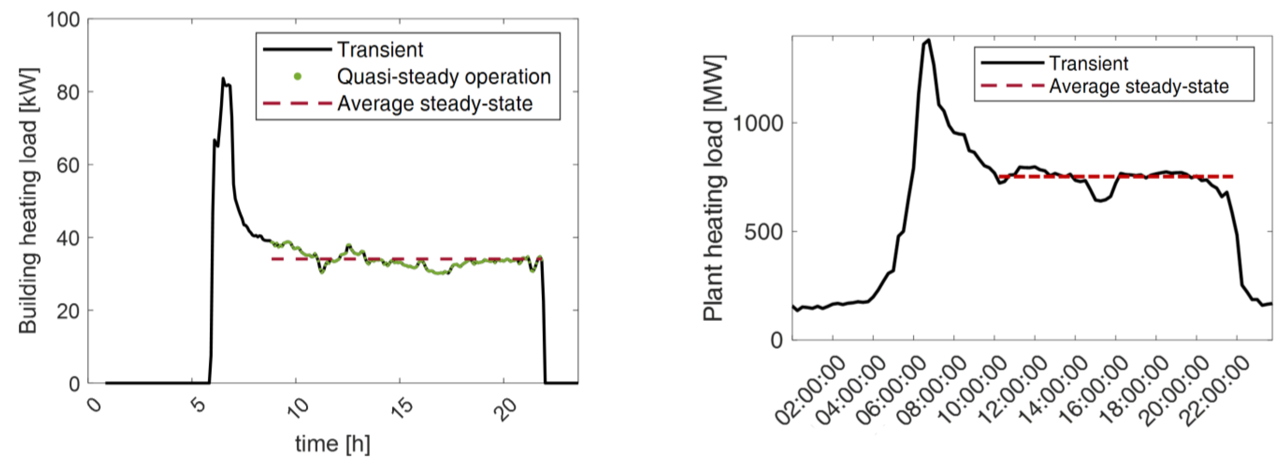
The thermo-fluid dynamic model of the network permits to estimate temperatures, pressures, and mass-flow rates within the network. It is based on the conservation equations of mass, momentum, and energy. The analysis is carried out in steady state conditions, since the main goal is to analyze the operation of the system at different base loads, while peak conditions that would require a transient simulation are out of the scope of the present work. The steady-state assumption can be made when focusing on the operation of the network on typical average steady conditions occurring after the morning start-up phase and lasting for each operating day. A representation of typical profiles of the heating load at building level and plant level is given in Figure 1, in which real profiles of a large-scale DH network located in Italy are reported. This network is mainly used for space heating purposes, while the supply of domestic hot water is limited to very few thermal users. The following considerations can be made:

• At the building level, the heating load profile reproduces a typical pattern in Mediterranean regions: in these areas, the heating devices of the buildings are shut down (as in the reported case) or attenuated during the night, leading to huge thermal requests in the morning when the systems are switched back on. Thus, the thermal transient occurring in the morning is significant, but limited to few hours of the day. On the other hand, after the start-up transient, an almost steady behavior is observed for the rest of the day until the system is shut down in the late evening. To have a better understanding of this aspect, the example reported in the figure has been tested using a self-developed algorithm to identify the steady-state operating conditions. The resulting steady-state operating points are reported with green dots in the figure, and the corresponding average steady-state is represented with a dashed red line. The main outcome of this test is that steady-state conditions can be identified for the majority of the day: in the presented case, they occur for more than 80% of all the on conditions.
• A similar trend can be observed at the plant level: in this case, the total heating load can be seen as a combination of all the heating loads of the buildings connected to the network, the thermal losses, and the dynamics of the network itself. The profile reported in the figure shows also in this case a low heating load during the night (due to shut down and attenuation of the different buildings), a consequent heating peak in the morning, and an approximate steady trend immediately after the morning start-up phase. Possible deviation from average conditions (like the small valley in the afternoon) are generally managed with thermal storages, while heating plants are typically operated with a steady load. Again, steady conditions can be observed for the majority of the time.

For the mentioned considerations, although DH generally has a dynamic behavior especially at the beginning of the day during the start-up transient and although this behavior is affected by significant seasonal patterns, some useful analyses (e.g., in the present work, the analysis on the influence of the location for the installation of a HP in a DH network) can be carried out by taking into account each steady-state occurring during each operating day of the year and representing the majority of the operating conditions. Other examples of analyses on DH conducted in the steady state can be found in the literature: Bahlawan et al. [33] have developed a diagnostic approach to evaluate possible faults in DH networks based on a steady-state analysis, using a similar approach identifying a point when the coefficient of variation of all physical quantities is lower than a fixed tolerance; similarly, Jakubeck et al. [34] have proposed a validated heat loss calculation algorithm presenting steady-state results.

The model adopted is one-dimensional and the complex structure of the network, constituted by pipes connected each other through junctions, is represented by means of the graph theory [35]. Each pipe is considered as a branch that starts in a node that represents the inlet section and ends in another node, representing the outlet section. The topology of the network is described by means of the incidence matrix $A$, which has as many as the number of nodes ($NN$) and as many columns as the number of branches ($NB$). The general element $A_{ij}$ assumes the value of 1 if the i-th node is the inlet node of the j-th branch, −1 if the i-th node is the outlet node of the j-th branch, and 0 if the i-th node and the j-th branch are not related to each other.

The equations that constitute the model are solved by means of the finite volume method [36], whose key step is the integration of the equations over a control volume (CV). On the one hand, continuity and energy equations are integrated over CVs including each node and half of the branch entering or exiting it. On the other hand, the integration of the momentum equation is performed over CVs, including a branch and the two delimiting nodes. Moreover, it is important to state the assumption of adiabatic and perfect mixing, applied to the streams converging in a junction: the temperature of all the flows exiting from the junction are assumed to be at the same temperature.

The integrated forms of continuity, momentum, and energy equations and their application to a DH network result in the following matrix formulation [37,38]:

$$A\cdot G+G_{ext}=0$$

(1)

$$G=Y\cdot A^{\mathrm{T} }\cdot P+Y\cdot \tau$$

(2)

$$K\cdot T=g$$

(3)

Equation (1) represents the matrix form of the continuity equation, where $G$ is a vector of dimensions $NB\times 1$ containing the mass-flow rate flowing in each branch of the network, and $G_{ext}$ is a vector $NN\times 1$ containing the mass-flow rates that are injected and extracted in the nodes (respectively at the substations and in the plants if the return network is considered).

Equation (2) is the matrix form of the momentum equation, in which $Y$ represents the fluid dynamic conductance matrix, of dimensions $NB\times NB$, $P$ is the vector $NN\times 1$ containing the pressure at each node, and $\tau$ is a vector $NB\times 1$ containing the pressure increase due to pumps.

These two equations make up the fluid-dynamic problem, with unknowns $G$ and $P$. In case of complex networks containing loops, this problem is solved by means of an iterative algorithm, fully detailed in Sciacovelli et al. [39].

Finally, Equation (3) represents the thermal problem. Specifically, $K$ is the $NN\times NN$ stiffness matrix, constructed adopting an upwind scheme [36] to associate face values to nodal values of temperature, $T$ is the vector $NN\times 1$ of the nodal values of temperature, representing the unknown of the problem, and $g$ is the known term vector $NN\times 1$, accounting for losses. As boundary conditions, mass-flow rates injected into the network and the corresponding water temperatures are imposed.

For validation purposes, model results are compared to experimental data in Figure 2. In particular, the supply temperature reaching four different substations belonging to different buildings connected to a small-scale DH sub-network located in Italy is represented; this network corresponds to a portion of the large-scale DH network analyzed in this paper as a case study in which a sufficient amount of experimental data are available. Model results are obtained through a steady-state application of the thermo-fluid dynamic model to the quasi-steady conditions identified in the analyzed network, while experimental measurements (which are taken every five minutes) are made available by the DH operator. It is possible to appreciate an excellent match between results and measures for all the on-conditions of the system. Concerning the off conditions (with zero heating load due to the night-time shutdown which is very common in buildings in Italy), which are highlighted in the figure with shaded areas, experimental measurements are not significant since the measurement system is typically located in technical rooms of the buildings which are unheated and exposed to outdoor conditions; thus, when the system is stopped, the water mass is subjected to temperature losses that are far higher than those occurring underground. Contrarily, when the system is active and the mass-flow rate continuously circulates, this aspect does not significantly affect the temperature solution because of the very short time the mass-flow rate circulates in the unheated environment. In these conditions, model results show good alignment with the temperature values recorded by the sensors. Further validation of the proposed thermo-fluid dynamic model of the network (in its complete transient formulation) has also been conducted by previous studies [38,40].

2.2. Heat Pump Model

The HP considered for the DH installation is an air-to-water HP with “source-return” [28] configuration: ambient air is used to preheat water in the return line of the network before it reaches the thermal/cogeneration plant, as illustrated in Figure 3. This layout guarantees a lower source-sink temperature gap with respect to other available configurations. Thus, the HP coefficient of performance (COP) is higher.

In order to represent the HP within the model, it is assumed that the mass-flow rate is extracted in a certain junction (node) and then reinjected at higher temperature in a new fictitious node, which is inserted downstream at a fixed distance. The mass-flow rate processed by the HP is constrained by the maximum value admitted by the device: if the HP is located on a branch whose total flow exceeds this threshold, only a portion of the flow rate is treated by the HP, while the remaining part bypasses the electric device and then it is mixed with the flow that has been heated up by the HP.

The temperature of the mass-flow rate that is reinjected into the system depends on (a) the inlet temperature, i.e., the extraction temperature, that consequently varies depending on the position of the HP, and (b) the COP of the machine. Its value can be derived from the definition on the COP of a HP, expressed by Equation (4), where $Q$ represents the useful heat and $W_{el}$ is the input work, which is constant.

$$\mathrm{COP}=\frac{\left|Q\right|}{\left|W_{el}\right|}$$

(4)

Since $Q=G_{HP}{c}_p\left(T_{ou{t}_{HP}}-T_{i{n}_{HP}}\right)$, being $G_{HP}$ the mass-flow rate elaborated by the HP (this value is limited by an upper boundary $G_{lim}$), $c_p$ the specific heat of water, $T_{out}{}_{HP}$ the water temperature at the outlet of the HP (corresponding to the water temperature at the injection node) and $T_{i{n}_{HP}}$ the water temperature at the inlet of the HP (corresponding to the water temperature at the extraction node), Equation (4) can be reformulated as:

$$T_{ou{t}_{HP}}=T_{i{n}_{HP}}+\frac{\mathrm{COP}\cdot W}{G_{HP}\cdot c_p}$$

(5)

The $\mathrm{COP}$ varies with the temperature of the cold source, i.e., ambient air, $T_C$, and the temperature of the hot sink $T_H$, taken equal to the mean between $T_{i{n}_{HP}}$ and $T_{out}{}_{HP}$, as reported in Equation (6). This makes the COP dependent on the solution $T_{ou{t}_{HP}}$ itself and Equation (5) non-linear.

$$\mathrm{COP}=\psi \frac{T_H}{T_H–-T_C}=\psi \frac{\mathrm{mean}\left(T_{i{n}_{HP}},T_{ou{t}_{HP}}\right)}{\mathrm{mean}\left(T_{i{n}_{HP}},T_{ou{t}_{HP}}\right)-T_C}$$

(6)

In Equation (6), the coefficient $\psi$ represents the second-law efficiency of the HP. This is a technical characteristic of the HP, expressed as the ratio between the effective COP, measured with an experimental test and the Carnot COP at those conditions. The second-law efficiency of the HP is kept constant throughout the analysis: in this case, the value of $\psi$ is considered equal to 0.34.

In order to evaluate $T_{ou{t}_{HP}}$ it is necessary to solve a system of nonlinear equations, made by Equations (5) and (6), where $T_{i{n}_{HP}}$ and $G_{HP}$ depend on the topology of the network and on the HP position and are evaluated by means of the thermo-fluid dynamic model.

2.3. Coupling District Heating and Heat Pump Models

In order to obtain a complete description of the operation of the system, the two described models need to be coupled. The full model, including both the thermo-fluid dynamic description of the DHN and the modeling of the LHP, can be summarized by the following steps:

• At first, a simulation of the supply line of the district heating network is performed. This simulation uses as input the mass-flow rates required by all the buildings of the network $G_u$, the share of mass-flow rate supplied by each plant $G_p$, and the supply temperature of each plant of the network $T_p^s$. These values represent the boundary conditions of the supply-simulation thermal problem. By applying the thermo-fluid dynamic model developed in Section 2.1 to the supply network, it is possible to obtain the temperature distribution along the whole supply line${\mathbf{T}}^{\mathbf{s}}$, besides the mass-flow rates and pressure distribution (for clarity, only the thermal part is discussed in this section, although the hydraulic part is also included in the simulation).
• The second step consists of a simplified modeling of the thermal users’ behavior. This step allows calculating the boundary conditions of the return network thermal simulation $T_u^r$(that are the input of the next step) by knowing the mass-flow rates required by the users $G_u$, their heating loads ${\Phi }_u$, and the supply temperatures of the thermal substations $T_u^s$ (which are part of the solution calculated at step 1 ${\mathbf{T}}^{\mathbf{s}}$).
• Once the boundary conditions of the return network thermal problem (namely the temperatures leaving each thermal substation $T_u^r$) are known, it is possible to run a simulation of the return line of the network, requiring as further input the mass-flow rates injected from the buildings $G_u$ and those extracted from the plants $G_p$. This is the step including the coupling with the heat pump model (being the heat pump considered with “source-return” configuration). Indeed, the temperature distribution along the return network ${\mathbf{T}}^{\mathbf{r}}$, which is the solution of the thermal simulation of the return network, is influenced in this case also by the presence of the heat pump, which is responsible for a temperature rise in the corresponding branch and needs to be accurately included into the return network simulation. Thus, the conditions described in Section 2.2 are imposed here: in the outlet node of the heat pump, there will be a Dirichlet boundary condition to fix its temperature equal to $T_{ou{t}_{HP}}$, evaluated according to Equations (5) and (6); it is worth highlighting again that this system of equations is non-linear, due to the dependency of the COP on the network temperatures themselves. Thus, the coupling and the solution of this step is non-trivial. Moreover, further non-linearities arise when considering the mass-flow rate $G_{HP}$ as not known a priori as assessed by the solution of the hydraulic problem, but evaluated depending on the thermal solution itself, as will be shown in Section 4.4. In this last case, some iterations are also needed to obtain the correct solution. In the end, this step allows evaluating the temperature distribution along the whole return network ${\mathbf{T}}^{\mathbf{r}}$.
• The last step allows evaluating the final heating load of the plants as ${\Phi }_p=G_p{c}_p\left(T_p^s-T_p^r\right)$. The total heating load of the plants will be reduced with respect to the case without heat pump because of the higher value of the return temperature $T_p^r$, included of the solution obtained at Step 3, in at least one of the plants.

The described model allows obtaining a complete thermo-fluid dynamic description of the DHN considering the installation of a LHP. A schematic of the full model is reported in Figure 4. The solution will be useful to estimate significant KPIs to assess the performances of heat pump installation in different points of the network. These KPIs are discussed in the next sections.

2.4. Exergy Analysis

In order to show how the positioning of a LHP within a DH network could affect the actual performances of the system, an exergy analysis is adopted. The parameter $\phi$ is defined as the ratio between the exergy of the fossil fuel that can be saved thanks to the HP ($\mathsf{\Delta }{E}_{fuel}$), which is the difference of the exergy of the fossil fuel before and after the installation of the HP, and the electric power required ($W_{el}$):

$$\phi =\frac{\mathsf{\Delta }{E}_{fuel}}{W_{el}}=\frac{E_{fuel, without HP}-E_{fuel,with HP}}{W_{el}}$$

(7)

The HP is supposed to be driven by electricity from renewable energy sources, thus its exergy contribution is not included when calculating the exergy saved into the numerator. It is instead taken into account in the denominator in order to normalize the savings.

Different HP configurations are compared by monitoring the parameter $\phi ;$ higher values of the coefficient indicate more advantageous configurations.

For the cogeneration plants, the exergy associated to the fuel consumption can be estimated using the second-law efficiency ${\eta }_{II}$ definition, reported in Equation (8). This value is assumed constant and equal to 0.56, which is the value given by the company managing the DHN analyzed.

$${\eta }_{I{I}_{CHP}}=\frac{E_{CHP}}{E_{fue{l}_{CHP}}}$$

(8)

In Equation (8), $E_{CHP}$ represents the exergy of the product, that is the temperature rise of the DH mass-flow rate in the cogeneration plant. For each plant, it is computed as:

$$E_{CHP}=G_{plant}\left(b_{out}-b_{in}\right)= G_{plant}{c}_p\left(T_{out}-T_{in}-T_0\ln \frac{T_{out}}{T_{in}}\right)$$

(9)

Therefore:

$$E_{fue{l}_{CHP}}=\frac{G_{plant}{c}_p\left(T_{out}-T_{in}-T_0\ln \frac{T_{out}}{T_{in}}\right)}{{\eta }_{I{I}_{CHP}}}$$

(10)

On the other hand, boilers have a constant first law efficiency, equal to $0.90$, as given by operators of the analyzed DHN. Hence, in order to compute the exergy of the fuel, it is possible to suppose that it is equal to its thermal power:

$$E_{fue{l}_{boiler}}\cong {\mathsf{\Phi }}_{fue{l}_{boiler}}= \frac{G_{plant}{c}_p\left(T_{out}-T_{in}\right)}{{\eta }_{I_{boiler}}}$$

(11)

In Equations (9)–(11), $G_{plant}$ represents the mass-flow rate processed by the plant, $c_p$ is the specific heat of the fluid, $T_0$ is the temperature of the reference environment, $T_{out}$ is the temperature of the water exiting the thermal plant, and $T_{in}$ is the temperature of the water reaching the plant. $T_{in}$, is estimated using the thermo-fluid dynamic behavior of the network. This estimation is carried out with the discussed numerical model.

2.5. CO₂ Emissions Reduction

The quantification of the environmental impact is completed by an estimation of the CO₂ that can be saved through the installation of the HP. The carbon dioxide emissions can be evaluated through the following equation:

$$m_{C{O}_2}=\frac{E_{C{H}_4} r_{C{O}_2/C{H}_4}}{H_i}$$

(12)

where $E_{C{H}_4}$ is the exergy of CH₄ (which can be directly related to the primary energy), $r_{C{O}_2/C{H}_4}$ is the CO₂ emission factor that can be estimated around 1.956 kg_CO2/Sm³_gas, and $H_i$ is the lower heating value, equal to 33.96 MJ/Sm³ for the natural gas. The carbon emission savings are obtained by subtracting the carbon dioxide emissions in the two cases (case without HP installation minus case with HP), which has been done for all the scenarios analyzed to compare the emissions savings in various HP locations.

2.6. Cost Savings

Lastly, an evaluation of the convenience of installing a LHP within the DH infrastructure is carried out by monitoring an economic KPI, defined as the unit cost of thermal production, which is labelled as $c$ and estimated dividing the total expenses (i.e., the expenses due to the fuel consumption and to the electricity required by the heat pump) by the thermal energy produced by the different plants (CHP, HOB, HP):

$$c=\frac{c_{C{H}_4}{E}_{C{H}_4}+c_{el}{W}_{el}}{E_{th}}$$

(13)

The specific costs for gas and electricity are taken from a database of IRENA [41] and referred to the year 2022, considering the EU ETS emission prices for fuel costs and the cost for electricity coming from renewable solar production.

3. Case Study

3.1. System Description

The topology and the building thermal demand are taken from a real case study consisting in a large-scale DH network (serving more than 6500 buildings) located in Northern Italy. In the selected system, typical winter demand is 1 GW, with peaks up to 1.4 GW. The main final use of the heating demand is space heating, while supply of domestic hot water is limited to very few users. Six thermal plants and storages satisfy the thermal demand of the network. The network can be considered as the integration of two interconnected parts: the transport network (whose illustration is provided in Figure 5) and the distribution network. The former connects the plants to multiple distribution networks, and it is characterized by larger diameters. The latter, instead, connects the transport network with various buildings located in the same area of the city, and it characterized by smaller diameters.

The network is supplied by pressurized hot water at 120 °C, while the return temperature varies from 50 °C to 70 °C, depending on the thermal load.

The storage available within the network, used for peak shaving, are not included in the study since the analysis as previously discussed is carried out in steady-state operations. Four plants are involved in the analysis: two CHP plants (labelled as CHP1 and CHP2) and two boilers (HOB1 and HOB2).

The analysis is performed considering the average plant heating load, which is equal to 305 MWt. The HP supplies the network with its nominal electric power, equal to 4 MWe. Thus, it can provide about 3% of the total thermal power depending on the COP. Despite the potential for the heating load to vary significantly during the year, this has a minor influence on the optimal positioning of the HP, which is instead more affected by how the heating load is distributed among the different plants. Moreover, the consideration of the average heat load allows for significant results even when considering the full annual operation, since it can be shown that $\phi \left(\overline{\mathrm{\Phi }}\right)=\overline{\phi }\left(\mathsf{\Phi }\right)$ because their relationship is nearly linear. These two aspects will be better addressed in the discussion section.

3.2. Analyzed Scenarios

To assess the convenience of installing the HP in different locations of the network, different configurations are analyzed representing various combinations of the possible production layout in terms of distribution of the heating load among the different plants:

• Cogeneration-based operation (Configuration 1): The thermal power is completely supplied by the two cogeneration plants CHP1 and CHP2 and by the newly installed HP. The operation selected is that CHP1 and CHP2 process 53% and 47% of the total mass-flow rate respectively.
• Cogeneration and heat-only boiler operation (Configuration 2): The thermal power is provided by cogeneration system and heat only boiler. Specifically, 63% of the total mass-flow rate is provided by cogeneration plants and 37% from boilers. This scenario refers to large demands that cannot be fully met by the cogenerators and less efficient production systems—e.g., heat-only boilers (HOB)—must be operated.
• The other configurations are characterized by off operations of the various plants (this could happen for various reasons, such as maintenance or fault). Specifically, the plants taken off in Configuration 3 to 6 are respectively CHP1 (Configuration 3), CHP2 (Configuration 4), HOB1 (Configuration 5), and HOB2 (Configuration 6).

The different distribution of the heating load among the different plants brings to different results in terms of convenience of installing the HP in one point of the network rather than another, which is evaluated by means of the various key performance parameters discussed in Section 2. To have a global view of what happens throughout the whole year of operation, an average scenario is analyzed, combining the different configurations for their respective operating time. This scenario combines some time the system operates in the condition of Configuration 1, some it operates as in Configuration 2, and the other configurations (Configuration 3 to 6) are characterized by off operations of the various plants. This allows a global yearly view assessment.

The average yearly operating conditions are estimated using an average coefficient, weighted on the yearly operating time of each configuration. Thus, a new coefficient $\overline{\phi }$ is defined to take into account the percentage of time $p$ of each configuration $i$:

$$\overline{\phi }={\displaystyle \sum }_{i=1}^{\# Conf.}{p}_i{\phi }_i$$

(14)

These six configurations are combined to estimate the average yearly operation with two different scenarios:

• Base-case: The installation of the HP along the return network brings an increase in the return temperature to one or more production plants. The mass-flow rate processed by each plant is kept unchanged with respect to the case without the HP. Consequently, the heating load of the production plants with higher return temperature decreases, regardless of whether the plant is a CHP or a HOB.
• Different mass-flow rate control strategy: In this second case, when the HP preheats the flow in the return line to the production plants, the mass-flow rate of the different plants are subjected to a control strategy and modified with respect to the base-case such that the CHPs are forced to work always at the same thermal power. If the HP preheats a water flow directed to the CHP, its mass-flow rate is increased so that the CHP thermal load is constant. The increased mass-flow rate also helps keeping temperatures lower, improving the COP of the device. Instead, the HOB mass-flow rate is decreased so that its thermal load decreases. This strategy results in a further total exergy reduction even when the HP is located in the proximities of a CHP plant, (in case of combined CHP-HOB operations). The heating load of the CHP plants is reduced only in the case HOBs are not in operation (e.g., as occurs in Configuration 1). This mass-flow rate control strategy can be applied only when there are not specific constraints on the network infrastructure (e.g., mass-flow rate congestion and fluid-dynamic bottlenecks).

4. Results and Discussion

4.1. Cogeneration-Based Operation

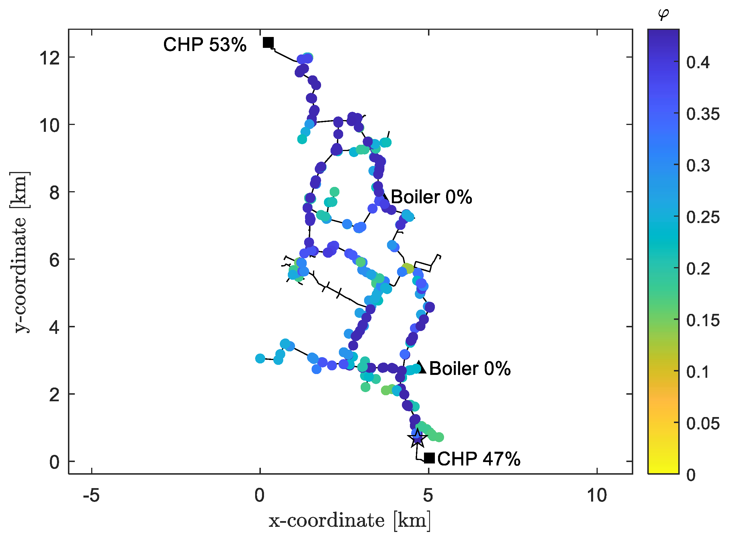
The first set of analyses aims at estimating the advantages given by the different locations of a large-scale HP in a cogeneration-based DH system. Here, specifically, as described in Section 3.2, CHP1 and CHP2 process respectively 53% and 47% of the total mass-flow rate. The results obtained from the simulation are presented in Figure 6. What stands out in the figure is that the best position for the HP is as close as possible to the cogeneration plant. This is true for three main reasons:

• If the HP is installed in the proximity of the plant, the distribution losses are lower. Oppositely, if the mass-flow rate is heated-up far from the production plant, the heat dispersion increases.
• The closer the HP to the plant, the lower is the inlet temperature $T_{in}$, due to the distribution losses on the return line. This results in a positive effect for the $\mathrm{COP}$.
• The mass-flow rate is higher in the branches that are closer to the plant. Therefore, given that the electric power of the LHP is fixed, and so is the thermal power, the temperature rise is lower. As a consequence, $T_{out}$ might be significantly reduced: this is a further and more relevant positive effect for the $\mathrm{COP}$. However, it is worth remembering that the mass-flow rate that the HP is able to process has a limit: if the branch exceeds this threshold, only a portion of the flow rate is treated by the HP and then it is mixed with the remaining part. This is the reason why comparable values of $\phi$ are obtained for all the cases with a sufficient large mass-flow rate.

For these considerations, the highest value of $\phi$, equal to $43.1\%$, shows up at node 367, that is the closest node to an operating cogeneration plant. This node is highlighted in Figure 4 with a star marker. Concerning the carbon dioxide emissions, according to Equation (12), the savings amount to $8.6 t_{CO2}/day$.

4.2. Cogeneration and Heat-Only Boiler Operation

When the thermal load is high, as described in Section 3.2, this is considered to be supplied with cogeneration (63% of the total mass-flow rate) and boilers (37% of the total mass-flow rate). Results of the simulation for this configuration are shown in Figure 7. The most interesting aspect is that the scale significantly changes. Close to CHP plant, the $\phi$ values have approximately the same order of magnitude of the previous case. In the proximity of boilers, the $\phi$ values are remarkably higher. This is because the mass-flow rate processed keeps unchanged before and after the HP installation therefore the adoption of the HP deals to a reduction in the heat supplied by the HOB. Second, HOB efficiency does not decrease when increasing the return temperature; differently than CHP, as shown by Equations (10) and (11). Therefore, as expected, if they are operating, it is convenient to use the HP close to the HOB thermal load.

In particular, for the same reasons previously mentioned—namely lower distribution losses and higher COP—the best position for the HP turns out to be the closest one to the boiler with the highest mass-flow rate. This happens at node 103, that ensures a $\phi$ value equal to $234.2\%$. The corresponding amount of CO₂ emissions reduction is of $46.6 t_{CO2}/\mathrm{d}\mathrm{a}\mathrm{y}$. This proves that reducing the thermal load of a boiler is far more effective than reducing the thermal load of a CHP plant.

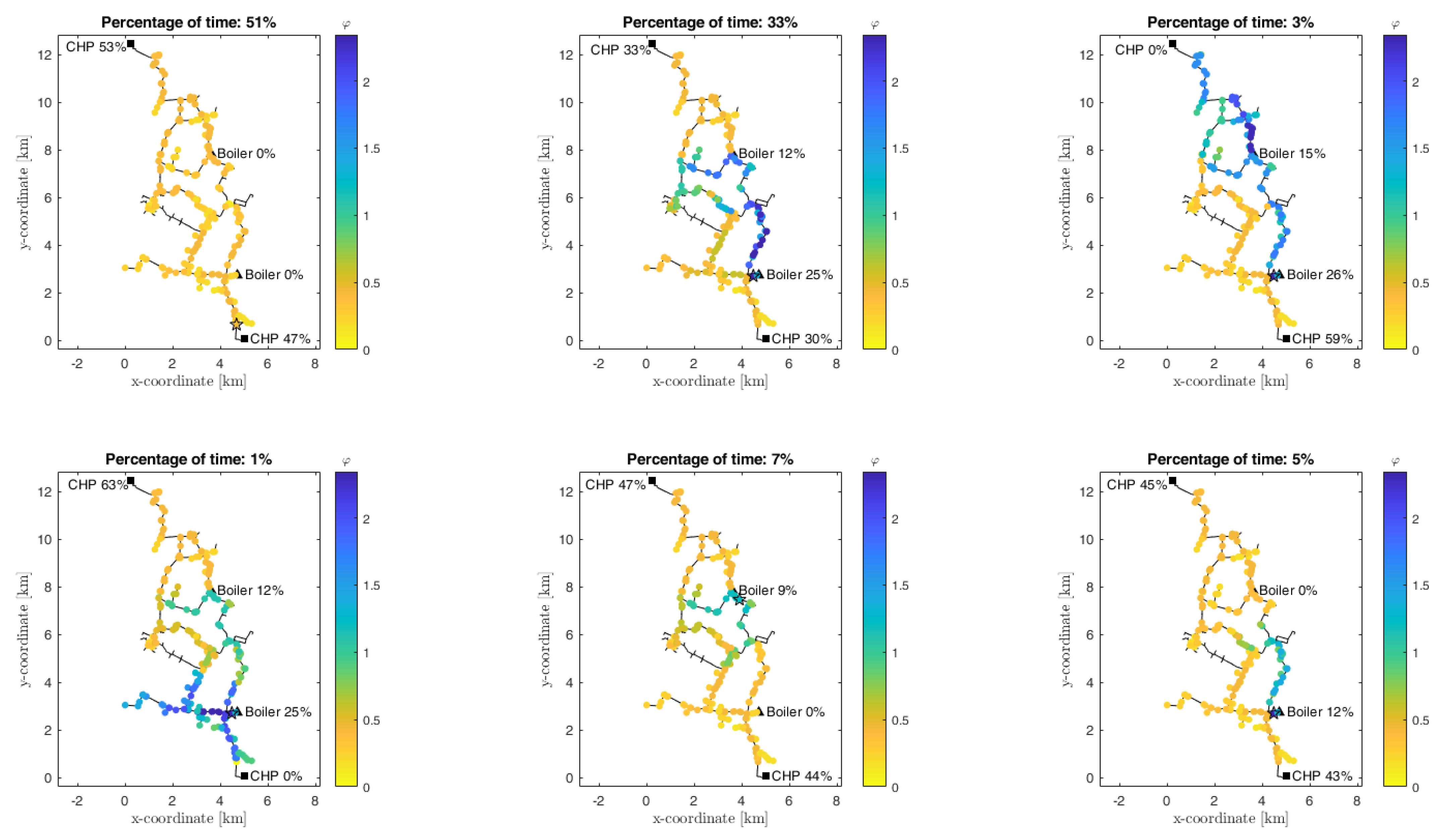
4.3. Average Operating Conditions

The previous analyses show that the differences among the various potential positions for the installation of a HP a complex DH network depend on how the thermal load is distributed among the different types of plants during the day. Here, the average yearly operating conditions are analyzed. The case reported here considers six different production assets: the two configurations described in the previous paragraphs (Configuration 1 and Configuration 2) and four configurations in which one plant at a time is turned off (Configurations 1 to 6). The results of each set-up are illustrated in Figure 8. The best location of the HP depends on how much each configuration works. Therefore, a percentage of time is fixed for each case, as reported in the figure.

The values of $\overline{\phi }$ for the proposed example are reported in Figure 9. An interesting aspect is that the best position for the HP obtained by averaging the various configurations (denoted in the figure with a star) does not correspond with any of the best positions of the single cases. Actually, it is located at node 383, in a branch that is connected both to the CHP and to the HOB. In this location, the temperature value in the return network—which is used as the inlet temperature for the HP and influences the COP—varies between 50.4 °C and 50.9 °C depending on the selected configuration (50.6 °C considering the average yearly operation). The corresponding value of $\overline{\phi }$ is equal to $116.5\%$.

Moreover, it is possible to estimate the CO₂ emissions that can be avoided in a whole heating season, which is extended from October 15th to April 15th in the location considered. If the HP is located in its optimal position they accounts for $4220 t_{CO2}/y$, which represents a reduction of about $3.3\%$ with respect to the total amount of emissions in a year without the power-to-heat device (that are about $126\cdot {10}^3 t_{CO2}/y$). This percentage strongly depends on the size of the HP, and it can be further enhanced by increasing its electric power. If the HP is installed close to CHP2 and to HOB2 the CO₂ reductions are respectively of $1560 t_{CO2}/y$ and $4058 t_{CO2}/y$. This would lead to a decrease in the CO₂ savings of −63.0% and −3.8% if placing the HP respectively close to the cogeneration and boiler plants instead of its optimal position considering the whole yearly operation.

Finally, considering the unit cost of thermal production, it is reduced from 115 €/MWh in the case the HP is not installed, to 111 €/MWh if installing the heat pump in its optimal position.

4.4. Mass-Flow Rate Control Strategy

As highlighted from the previous findings, it appears to be significantly more favorable to reduce the thermal load of a HOB (if it is working), by installing the large-scale HP in its vicinities, since it is generally less efficient than a cogeneration plant.

On the other hand, the reduction in the thermal load of a cogeneration plant does not give equally positive results. Indeed, in these cases the coefficient $\phi$ dramatically drops from $234.2\%$ to $44.2\%$ (these values refer to the example in Section 4.2). Based on these results, a different mass-flow control strategy is analyzed: the CHP are forced to work always at the same thermal power while the HOB thermal load decreases, as detailed in Section 3.2.

Considering the mass-flow control strategy, the $\phi$ coefficient throughout the DH network for each configuration is reported in Figure 10. Apart from the first case, in which the boiler is not active and there is no possibility to reduce its thermal load, all the other configurations can obtain a greater average value of $\phi$. Note that, due to the control strategy, the mass-flow rate percentages reported in the figure are no more exact, but they are useful to give upper or lower mass-flow rate boundaries.

Figure 11 shows the weighted coefficient $\overline{\phi }$, obtained according to Equation (13). In this case, the maximum $\overline{\phi }$ is about $133.1\%$, greater than the case without control strategy (which was $116.5\%$) but in the same position. Generally, it can be observed that the value of $\overline{\phi }$ within the network is higher than the previous case: its average value passes from $50.3\%$ to $96.8\%$. This is because, by applying the control strategy discussed, more positions become attractive for the prospective installation of a power-to-heat device.

Regarding the CO₂ emissions, by applying the mass-flow rate control strategies it is possible to obtain a reduction of $4823 t_{CO2}/y$($-3.8\%$ with respect to the case without HP) by locating the HP at its best position, $4376 t_{CO2}/y$ near the cogenerator and $4298 t_{CO2}/y$ near the boiler. Consequently, potential CO₂ savings of respectively 9.3% and 10.9% risk being lost if placing the HP close to the CHP or the boiler rather than at its optimal position, which must be evaluated considering the average yearly operation. Comparing the reduction obtained in the case of mass-flow control strategy, improvements have been achieved in all the cases, but the most significant improvement is achieved in the proximities of the CHP plant, where the previous strategy performed poorly.

Finally, also the unit cost of thermal production drops to 110 €/MWh.

It is worth mentioning that the possibility to apply this mass-flow rate control strategy is strictly dependent on the network configuration and on its operating condition. In the case analyzed, there were not specific problems of mass-flow congestion within the pipelines of the network. For other applications, these limitations must be taken into account and the shift of mass-flow rate to the boilers can be operated only until the pipeline threshold is reached.

4.5. Comparison and Discussion

A comparison of the different positioning in terms of CO₂ emissions is given in Figure 12. To have a global view of the potential benefits, results are referred to the average yearly operation and are reported both for the base-case and for the second scenario with mass-flow rate control strategy. From this figure, it is possible to see that the CO₂ emission reduction that can be achieved through the installation of the HP is always greater when the mass-flow rate control strategy is applied, since in this case more positions become significant for the installation of the device. In the best position, the installation of HP using the mass-flow rate control strategy brings to a reduction in the yearly CO₂ emissions of 4823 $t_{C{O}_2}/y$), which represents a −3.8% reduction compared with the case without HP.

In the case where no control strategy is applied (e.g., when it is not possible due to the constraints and the possible bottlenecks in the network), using an approach that allows estimating the best position for the installation of the HP becomes even more relevant because the different savings of the various locations are higher. Indeed, the best position for the HP—corresponding to an intermediate position—brings to a CO2 emissions reduction of about 4220 $t_{C{O}_2}/y$ (−3.3% with respect to the case without HP), while potential CO₂ savings of 63.0% risk to be lost if misplacing the HP close to the CHP plant (corresponding to a CO₂ reduction of 1560 $t_{C{O}_2}/y$), despite this plant being in operation for most of the time; this potential reduction would be instead of 3.8% if placing the HP close to the boiler (corresponding to a CO2 reduction of 4058 $t_{C{O}_2}/y$).

Finally, a summary of the values assumed by the different parameters adopted in the analysis in different locations of the network (i.e., the best location, near CHP2, and near HOB1) are reported in

Table 1. Summary of the values assumed by the different parameters adopted in the analysis in different locations of the network.

Average Yearly Value		KPI
		$\mathit{\phi }$	CO2 Reduction	Cost Savings
Base-case	Near CHP2	43%	$1560 t_{CO2}/y$	0.8%
	Near HOB1	112%	$4065 t_{CO2}/y$	2.7%
	Best position	117%	$4222 t_{CO2}/y$	2.8%
With flow control	Near CHP2	121%	$4376 t_{CO2}/y$	2.9%
	Near HOB1	118%	$4298 t_{CO2}/y$	3.0%
	Best position	133%	$4823 t_{CO2}/y$	3.2%

. The values reported quantify:

• The exergy parameter $\phi$ defined in Equation (7) and representing the ratio between the exergy of the fossil fuel that can be saved thanks to the HP and the electric power required.
• The CO₂ reduction which can be obtained as the difference between the CO₂ emissions obtained in the scenario without the installation of the HP and the CO₂ emissions achieved using the HP in the different cases, i.e.,: $m_{C{O}_2}^{without HP}-m_{C{O}_2}^{with HP},$ calculated according to Equation (12). No emissions are considered for the electricity needed by the HP, since it is supposed to be driven by renewable sources in this scenario.
• The cost savings that can be achieved through the installation of the HP. This is calculated as $\frac{c^{without HP}-c^{with HP}}{c^{without HP}}$, where the specific operating costs are evaluated using Equation (13). In this case, both costs for natural gas needed by HOBs and CHPs and the cost for electricity from renewables are considered. The investment cost is not included in the computation since it has been found to be negligible: considering the investment costs reported in [42,43] and the expected lifetime [43], it impacts cost savings of less than 0.1%.

For all the parameters reported in the table, higher values correspond to more favorable situations. Thus, according to the results, locating the HP in the right position assumes more and more relevance, especially in the case in which flow control strategies cannot be applied due to restrictions or bottlenecks in the network.

The installation of a HP in a DH network can be seen as a cost-effective way to integrate renewable sources in the DH supply. Thus, the convenience of installing a LHP within an existing DH network is clearly dependent on the availability of renewable sources in the considered area. As a consequence, the values assumed by the different parameters may significantly vary when electricity from renewable energy sources is not available. To give more generality to the results, a similar analysis is repeated considering a further scenario in which only 50% of the yearly electricity needed by the HP is supplied with renewables, while the remaining part is obtained by CHP plants. Of course, in this case the advantages tend to decrease, but the trend (depending on the positions and on the flow control strategy) remains the same. In the best position, the CO₂ reduction decreases to 1006 $t_{CO2}/y$ in the base-case and 1607 $t_{CO2}/y$if applying the mass-flow rate control strategy; concerning cost savings, these are of 0.5% and 1.0% in the two different scenarios.

Finally, the relevance of adopting an average heating load for the analysis is demonstrated. This is achieved by repeating the simulations of the base-case with a higher heating load, set to about 600 MW and corresponding to the maximum steady-state condition identified during a year of operation in the selected case-study. The $\overline{\phi }$ coefficient throughout the network corresponding to this higher heating load is represented in Figure 13. The values are lower with respect to the operation at 305 MW not only because of the higher temperatures on the return network (in this case, in the best position of the HP, the return temperature taken as input of the electric device is about 64.7 °C on average, while in the previous case it was 50.6 °C), resulting in lower values of the COP, but mainly because the heating load provided by the HP has a lower share with respect to the total heating load since the electric power is fixed. Nevertheless, the trend of $\overline{\phi }$ among the different positions is similar, since it is mainly associated with the different share of the heating load among the various plants rather than on the absolute value of the heating load itself. For this reason, the best position is always the same.

Finally, a black-box methodology is developed to quickly estimate the average $\overline{\phi }$ coefficient corresponding to a different heating load. This model is built by elaborating all the results (temperatures in critical points of the network, temperature increase given by the HP) obtained with the average heating load, equal to 305 MW, in the cases without and with the installation of the HP. This makes it possible to very quickly evaluate the $\phi$ value corresponding to a situation with a different heating load $\mathsf{\Phi }$. This model is validated by comparing the $\overline{\phi }$ values obtained from the model to those achieved with the full simulation with the maximum steady-state heating load (about 600 MW): the relative error is very small, less than 0.1%. This model is then used to estimate the $\overline{\phi }$ coefficient for all the values of steady-state heating load of the selected case-study over the year. The load duration curve of the network considered is reported in Figure 14a and it can be seen that the average heating load $\overline{\mathrm{\Phi }}$ is about 305 MW. In Figure 14b, the values of $\overline{\phi }$ corresponding to each $\mathsf{\Phi }$ value are reported. It can be seen that the average $\overline{\phi }$ value obtained with the analysis discussed in the previous chapters using the average steady-state heating load $\overline{\mathrm{\Phi }}$ is $\overline{\phi }\left(\overline{\mathrm{\Phi }}\right)=1.1653$ and is very well aligned with the value that would have been obtained with a full analysis $\overline{\overline{\phi }\left(\mathsf{\Phi }\right)}=1.1693$. The relative error is less than 0.4%, proving that not only the trend along the various point of the network is the same, but also that the absolute values assumed by the parameters are significant for representing the average yearly operation. This is related to the nearly linear behavior of $\mathsf{\Phi }\left(\phi \right)$.

5. Conclusions

LHP installations within DH networks are among the main strategies to improve the system efficiency and to reduce carbon dioxide emissions.

The paper proposes a methodology to analyze how the advantages provided by the installation of LHPs in existing large DH networks can vary considering different potential locations for the installation of the device. The proposed approach combines: (a) a steady-state thermo-fluid dynamic model of the network; and (b) a model of the HP that considers a variable COP and a limit on the mass-flow rate that can be treated. The comparison of the different positions is carried out by means of exergy considerations on the results provided by the integrated model. Moreover, CO₂ emissions and production costs are proposed as further KPIs.

An application to a real DH network is proposed. The potential benefit is quantified through the following parameters: (a) $\phi$, representing the ratio between the exergy of the fossil fuel that can be saved thanks to the installation of a HP and the electric power required; (b) the CO₂ emission reduction; (c) the unit production cost.

By analyzing the results, it turns out that the potential benefit is strictly dependent on the adopted plant configuration. Regarding the influence of the positioning, in the case of a cogeneration-based system, it results to be more convenient to collocate the HP in the immediate vicinity of the CHP plant, due to distribution losses and COP-related reasons. On the other hand, if a boiler is operating within the system, it turns out that reducing its thermal load is significantly better: therefore, if the mass-flow rates processed are not changed, the HP should be located in its proximities (because it reduces the boiler supplied heat). Thus, to have a global view, it is worth to consider the average operating conditions over a year. By doing this, the best position for the HP results to be in an intermediate position, which allow a CO₂ emissions reduction of about $4220 t_{CO2}/y$ ($-3.3\%)$if a HP of $4 \mathrm{MWe}$ is used. Potential CO₂ savings of 63.0% can potentially be lost if misplacing the HP close to the cogeneration plant (corresponding to a CO₂ reduction of $1560 t_{CO2}/y$), despite it is the plant that works for the majority of the time; this reduction would be 3.8% if placing the HP close to the boiler (corresponding to a CO₂ reduction of $4058 t_{CO2}/y$).

Finally, a further analysis is performed by considering a different mass-flow rate control strategy in order to improve the advantages provided by the installation of a HP. This is possible in the case of networks and operating conditions in which there are no specific problems of flow congestion. The mentioned control strategy aims to reduce the boiler load, although the HP is located on the return line toward a cogeneration plant. This is achieved by increasing the mass-flow rate of the CHP according to its return temperature and by decreasing the boiler mass-flow rate. In this way, the CHPs are kept at a fixed thermal load, while the boiler load is reduced despite its return temperature does not increase. This helps enhancing the advantages provided by the installation of a HP within the system, by increasing the saved carbon dioxide emissions up to $4823 t_{CO2}/y$ $\left(-3.8\%\right)$ with respect to the case without HP. In this case, if the HP is not located at its best position but close to the cogeneration plant or to the boiler, the potential CO₂ savings reduce by 9.3% and 10.9% respectively.

To sum up, it can be stated that the outcomes of this study are promising in terms of reduced pollutant emissions guaranteed by the installation of a LHP driven by renewable sources within an existing DH network. The approach discussed in this work represents a powerful tool to compare different potential locations for installation and to reduce even more the carbon dioxide emissions.

As regards possible developments, the CO₂ emissions monitoring could be performed under variable excess of electric power. Furthermore, the model could be extended to also take into account the distribution losses in the electric grid.