Article

RAC-GAN-Based Scenario Generation for Newly Built Wind Farm

1
Economic and Technological Research Institute of State Grid Inner Mongolia Eastern Power Co., Ltd., Hohhot 010020, China
2
School of Electrical Engineering, Northeast Electric Power University, Jilin 132012, China
*
Author to whom correspondence should be addressed.
Energies 2023, 16(5), 2447; https://doi.org/10.3390/en16052447
Submission received: 30 November 2022 / Revised: 16 January 2023 / Accepted: 1 March 2023 / Published: 3 March 2023
(This article belongs to the Special Issue Advances in Multi-Energy Systems and Smart Grids)

Abstract

:
Due to the lack of historical output data of new wind farms, there are difficulties in the scheduling and planning of power grid and wind power output scenario generation. The randomness and uncertainty of meteorological factors lead to the results of traditional scenario generation methods not having the ability to accurately reflect their uncertainty. This article proposes a RAC-GAN-based scenario generation method for a new wind farm output. First, the Pearson coefficient is adopted in this method to screen the meteorological factors and obtain the ones that have larger impact on wind power output; Second, based on the obtained meteorological factors, the Grey Relation Analysis (GRA) is used to analyze the meteorological correlation between multiple wind farms with sufficient output data and new wind farms (target power stations), so that the wind farm with high meteorological correlation is selected as the source power station. Then, the K-means method is adopted to cluster the meteorological data of the source power station, thus generating the target power station scenario in which the cluster information serves as the label of the robust auxiliary classifier generative adversarial network (RAC-GAN) model and the output data of the source power station is considered as the basis. Finally, the actual wind farm output and meteorological data of a region in northeast China are employed for arithmetic analysis to verify the effectiveness of the proposed method. It is proved that the proposed method can effectively reflect the characteristics of wind power output and solve the problem of insufficient historical data of new wind farm output.

1. Introduction

With the increasing depletion of fossil resources and the aggravation of environmental pollution problems, renewable energy has been vigorously developed. In recent years, renewable energy such as wind power is connected to the distribution grid. However, the uncertainty of renewable energy and its high penetration to the grid have brought huge challenges. Due to the insufficient historical data of new wind power stations, it is difficult to evaluate their operation performance. Therefore, scenario generation is of great importance. Most scenario generation methods require a number of training samples, which is difficult to collect for new power plants, so the analysis of neighboring wind farms with high similarity to new wind farms is a possible way to assist scenario generation.
A crucial factor that restricts the reasonableness of wind power output scenario generation is the insufficiency of operational data, which may be affected by new construction, expansion, or renovation of the stations. Therefore, it is necessary to explore a new method to analyze the correlation between the newly built wind farms and their neighboring wind farms and gain enough output data [1]. Most of the existing literature focuses on historical output data. For instance, there is a study in which a time-varying regular vine mixed Copula model is developed to analyze the Spatio-temporal correlation between multiple wind farms [2]. Meanwhile, some studies incorporate a non-separable covariance function in the scenario generation method, thus capturing the complex correlations between the Spatio-temporal components of wind power generation [3]. In addition, the Mutual Information, Spearman, and Kendall correlation coefficients are adopted in the correlation analysis of multi-wind farms with good results [4]. However, besides the historical output data, other factors such as time-series data of multiple meteorological features should be considered, for the consistency of its changing trends plays an important role in the correlation analysis of different wind farms, which has not been discussed in the current studies.
As for the renewable energy scenario generation, the current main idea is to generate new samples similar to the historical output scenarios after learning a given number of historical output data [5]. According to whether it is necessary to assume the probability distribution obeyed by the actual output data, the existing stochastic scenario generation methods can be divided into the explicit density model and the implicit density model [6]. The explicit density model requires an artificial assumption of the probability distribution obeyed by the output data, but the probability distribution obeyed by the wind power output data is usually unknown and difficult to model accurately with mathematical formulas, which leads to the inapplicability of the explicit density model to the wind power output scenario generation [7]. Therefore, generative methods that do not require probability distribution assumptions, such as variational autoencoders and generative adversarial networks, have been widely used in power system scenario generation. Some studies have proposed a GAN-based joint scenario generation method for wind and photovoltaic power generation [8]. In addition, a Gibbs sampling-based dynamic method is proposed in a study to overcome the difficulty of generating scenarios for multi-renewable energy plants [9]. Although the above literature analyzes a large amount of historical actual output data, the influence of meteorological features on the generation of wind power output scenarios has not been analyzed, and little research has been conducted on the generation of output scenarios for newly built wind farms.
To address the above problems, this paper proposes a scenario generation method based on RAC-GAN. First, in order to determine what meteorological information has a larger impact on wind power output, the Pearson correlation coefficient is used to screen multiple meteorological features. Second, based on the above screened meteorological features, the GRA method is adopted to analyze multiple wind farms with sufficient data close to the target power station, and thus the wind farm with the highest correlation is selected as the source power plant. Then, the K-means method is adopted to cluster the historical meteorological data of the source power plant, and the cluster information is used as the label of the robust multi-label generation adversarial network to generate scenarios based on the output data of the source power plant. Finally, the actual wind farm output and meteorological data of a region in northeast China are employed for arithmetic analysis to verify the effectiveness of the proposed method. The probability distribution characteristics and three evaluation indexes are used to analyze the generated results, and the proposed method in this paper can better generate scenarios for new wind farms and fill the historical data gap of new wind farms.

2. Selection of Source Power Station Based on GRA

2.1. Screening of Meteorological Features Considering the Correlation of Wind Power Output Influencing Factors

Wind power output may be affected by several factors such as wind speed, wind direction, temperature, humidity, pressure, and historical wind power. The Pearson correlation coefficient is also called the Pearson product-moment correlation coefficient. As one of the most commonly used linear correlation coefficients, it can analyze small local differences in patterns [10] without normalizing the wind power output data, which makes it a better way to analyze the correlation between the wind power output and various meteorological categories. The equation, denoted as R, is used to reflect the degree of linear correlation between two variables. The Pearson correlation coefficient quantifies the correlation between variables on the basis of covariance, which is calculated as follows:
R = c o v ( X , Y ) σ X σ Y = i = 1 n X i X Y i Y i = 1 n X i X 2 i = 1 n Y i Y 2
In the equation, R denotes the correlation coefficient of X and Y . c o v ( X , Y ) denotes the covariance of the two variables. X and Y denote the standard deviation of σ X and σ Y , respectively. The larger the absolute value of the correlation coefficient with an R -value between −1 and 1, the stronger the correlation between the variables, which is usually judged by the strength of the correlation of the variables in Table 1 [11].
The Pearson coefficient can effectively analyze the influence of each factor on wind power output. The absolute values of Pearson coefficients for each factor and wind power output are shown in Figure 1.
Figure 1 shows the Pearson coefficients between wind power output and various meteorological factors such as wind speed and wind direction. The first row of Figure 1 indicates the correlation between wind power output and each meteorological factor. It indicates that wind speed is the most direct and fundamental factor in determining wind power output. In addition, an analysis of the correlations using multiple years of data found that the correlation can vary slightly year by year but does not change the overall level of correlation. Wind speed was selected as a meteorological feature for the analysis.

2.2. Source Power Station Determination Considering the Consistency of Meteorological Data Trends

2.2.1. Steps of GRA

A measure of the magnitude of the correlation between the meteorological data of two wind farms over time or with different objects is called the correlation degree. During the system development process, two factors will be considered to be highly correlated if their changing trends are consistent, i.e., the degree of synchronous change is high. Conversely, the correlation degree is low [12]. GRA is a method to measure the degree of correlation between factors based on the degree of similarity or dissimilarity of their development trends, i.e., the “GRA”. According to the above-mentioned, wind power output is mainly influenced by wind speed, and the historical wind speed of multiple wind farms in a specific region has certain similarity. Therefore, in this paper, the GRA method is used to analyze the wind speed correlation between multiple wind farms and the target power station. The steps for selecting the source power station are as follows.
(1)
Construction of meteorological data set
The wind speed time series data selected above are used as the data set, and each scenario day is regarded as a feature vector. In this paper, 12 months of historical data in the year of 2014 are selected as the training set, and the eigenvector X i equation is constructed based on the mean value of wind speed for each historical day as well as the wind speed at each moment.
X i = F 1 i , F 2 i , , F g i , , F a v i
In this equation, F g i is the wind speed at the g t h moment of the i t h day; F a v i is the average wind speed on the i t h day.
(2)
Normalization of data
The wind speed data were normalized as follows [13].
x = x x m i n x m a x x m i n
In the equation, x , x m i n , and x m a x are the arbitrary values in the original data, the minimum values in the original data, and the maximum values in the original data, respectively; x is the normalized data. The normalized eigenvectors of the target power station and each neighboring power station are as follows:
x 0 i = x 0 i ( 1 ) , x 0 i ( 2 ) , , x 0 i ( n ) ,
x j i = x j i ( 1 ) , x j i ( 2 ) , , x j i ( n ) ,
In this equation, x 0 i is the eigenvector of the target power station on day i . x j i is the eigenvector of the i t h historical day of the j t h proximity power station. x 0 i ( n ) refers to the eigenvector of the target power station, and x j i ( n ) refers to the n t h element of the i t h historical day of the j t h proximity power station.
(3)
Calculation of correlation degree
Calculate the number of correlation coefficients between x 0 i and x j i at the n t h component, respectively.
ξ i ( n ) = m i n i m i n n Δ + r m a x i m a x n Δ Δ + r m a x i m a x n Δ
In the equation, ξ i ( n ) is the number of correlation coefficients. Δ = x 0 ( n ) x i ( n ) . r is the resolution factor, generally taken as 0.5. As there are many scattered correlation coefficients that are not easy to compare, they are generally processed by means of averaging. The GRA between x 0 i and x j i is defined as follows [14]:
R i = 1 N n = 1 N ξ i ( n )
In this equation, N is the total number of correlation coefficients for each component.

2.2.2. Selection of Source Power Station

Six actual wind farms in northeastern China are selected, and the longitude and latitude of the wind farms are shown in Table 2.
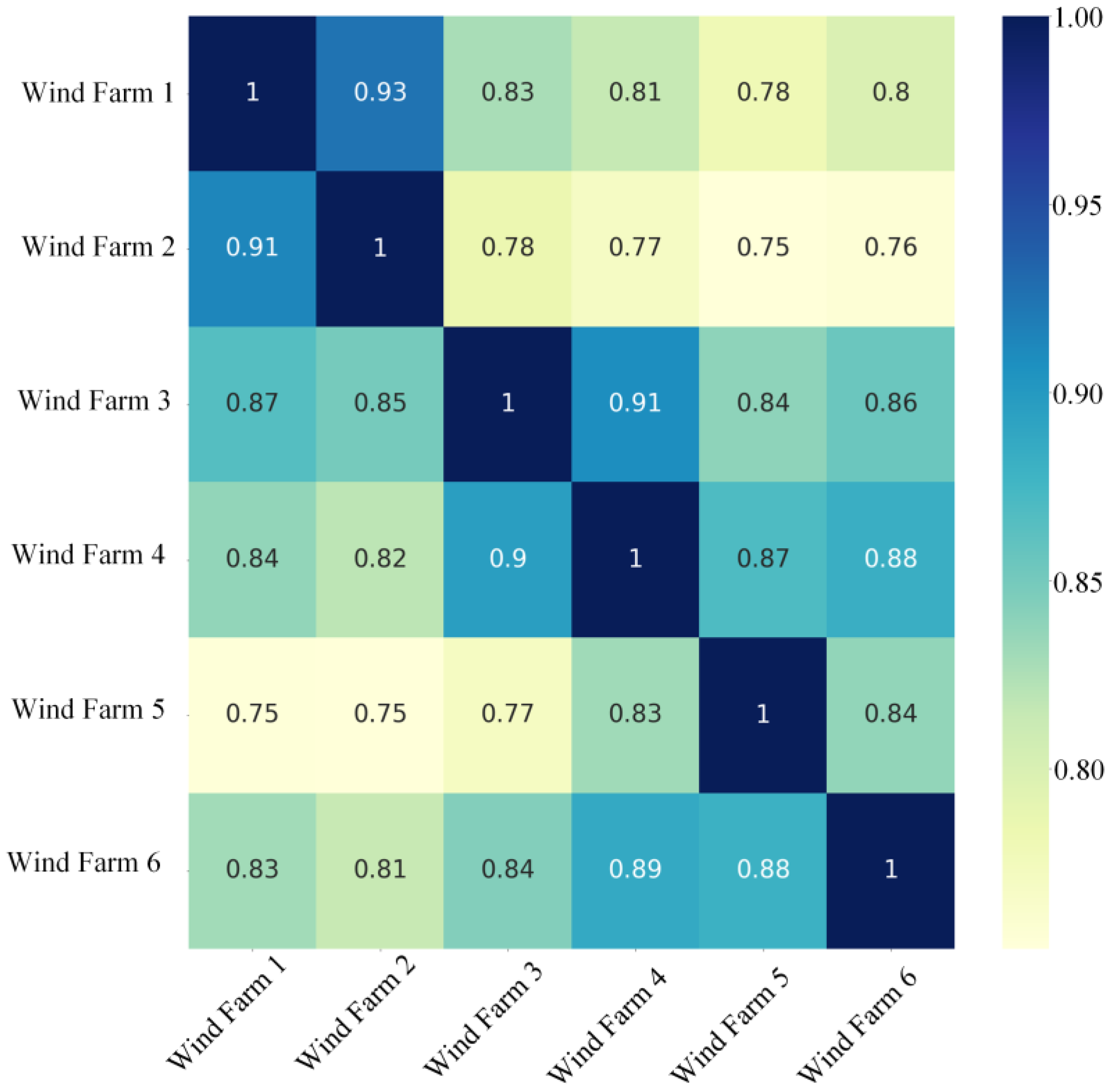
In the table above, assuming that Wind Farm 1 is a newly built power station with sufficient meteorological data but no output data, experiments are conducted with the GRA method based on the historical wind speed and other meteorological data, and the results captured are shown in Figure 2.
As can be seen from the overall trend of the data in Figure 2, the GRA values of the neighboring wind farms are greater than 0.75, which is a high level of similarity. It can prove that the historical wind speed temporal trends among multiple neighboring wind farms in a specific geographic area are consistent, while the wind farm with the highest consistency with the target power station is Wind Farm 2, with a GRA value of 0.93. Since wind speed is the most direct factor affecting wind power output, Wind Farm 2 can be selected as the source power station for the generation of wind power output scenarios for newly built power plants.

3. RAC-GAN-Based Scenario Generation of Wind Power Output

3.1. Clustering of Meteorological Historical Data Based on K-Means Method

Since the wind power output is mainly determined by the wind speed, the transformation of wind speed and wind power output can be described by the following formula [15]:
P W ( v ) = 0 , 0 v v in P W T v v in v r v in , v in < v v out P W T , v r < v v out 0 , v out v
In the formula, v is the wind speed; P W T is the rated power of the wind turbine; v r is the rated wind speed; v in is the cut-in wind speed; v out is the cut-out wind speed.
It can be seen in the formula that the wind speed is the most direct and critical factor affecting wind power output. The algorithm clustered by K-means is used to classify the historical meteorological scenarios and model the wind power output of the source power plants corresponding to the dates within different meteorological categories, with the obtained information of the clusters as the labels and RAC-GAN as the method for scenario generation. The basic unit of clustering on the time scale is the day, and each unit contains the meteorological data of that day. Altogether, the data cover 365 days in a whole year, and each scenario contains 24 h. Eventually, k typical meteorological categories are captured during the clustering process.
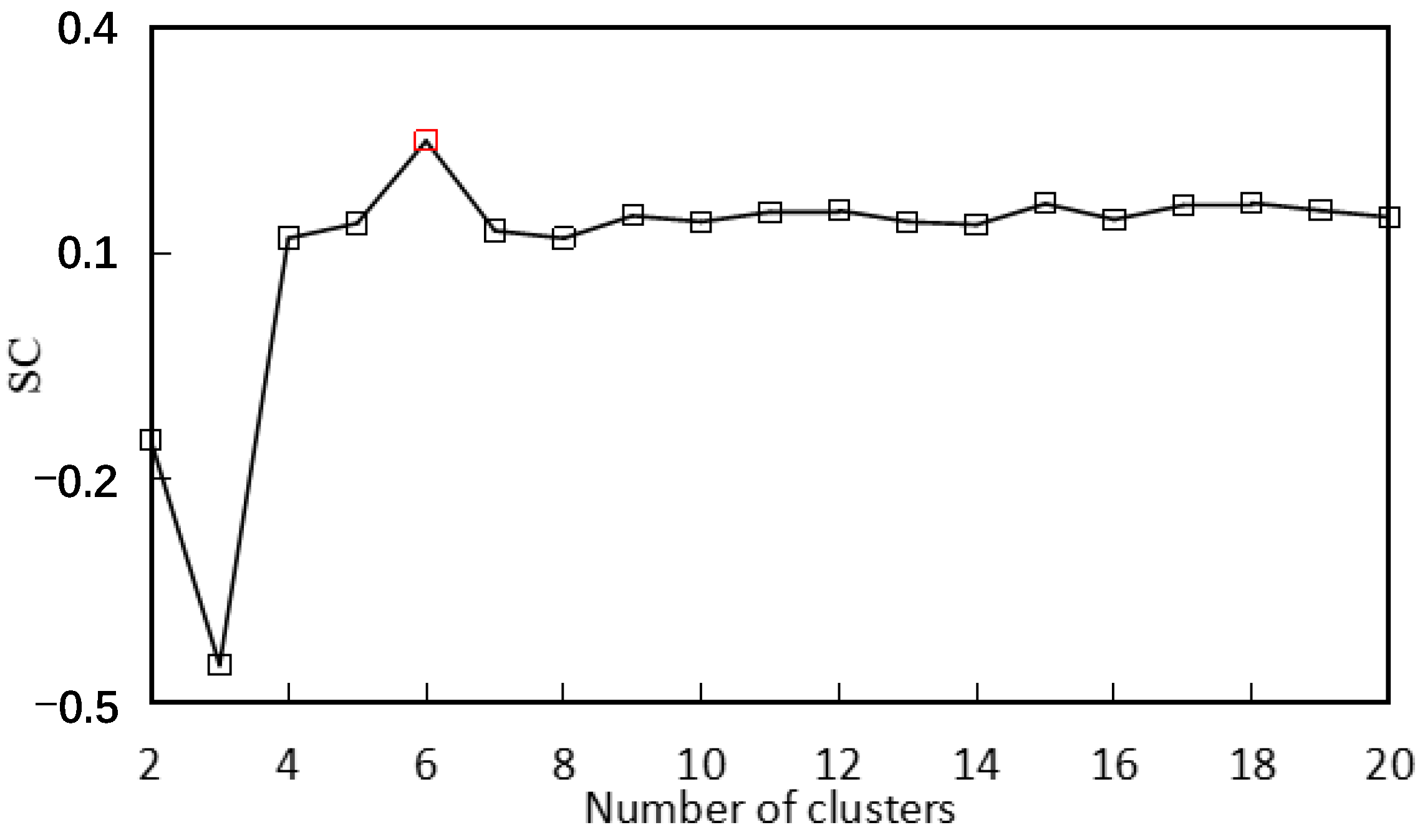
The clustered meteorological data set used in this paper is an unlabeled data set, and the categories of the data are not given in advance. Therefore, the internal indicators of clustering were chosen to evaluate the clustering results when selecting the clustering indicators. In this paper, the Silhouette Coefficient (SC) clustering index is selected to quantitatively analyze the clustering effect, and it determines the optimal number of clusters, following by the principle that ‘the higher the intra-cluster similarity and the lower the inter-cluster similarity, the better the clustering effect’. Assuming the data set has m samples k clustered into m classes, the number of clusters should not exceed 20 according to historical experience, i.e., K [ 2 , 20 ] [15]. The equation for calculating the above metric is as follows:
s ( k ) = b ( k ) a ( k ) m a x { a ( k ) , b ( k ) }
In this equation, b ( k ) is the minimum average distance from sample k to the samples of other clusters, and the larger b ( k ) is, the less sample k belongs to other clusters. a ( k ) is the average distance from the sample to other samples in the same cluster, and the smaller a ( k ) is, the more reasonable it is for sample k to be classified into this class. s ( k ) should have a value between [−1, 1], which means the closer it is to 1, the more reasonable the sample clustering is; the closer it is to −1, the more reasonable it is for sample k to be classified into other classes; the closer it is to 0, the more reasonable it is for sample k to be on the boundary.
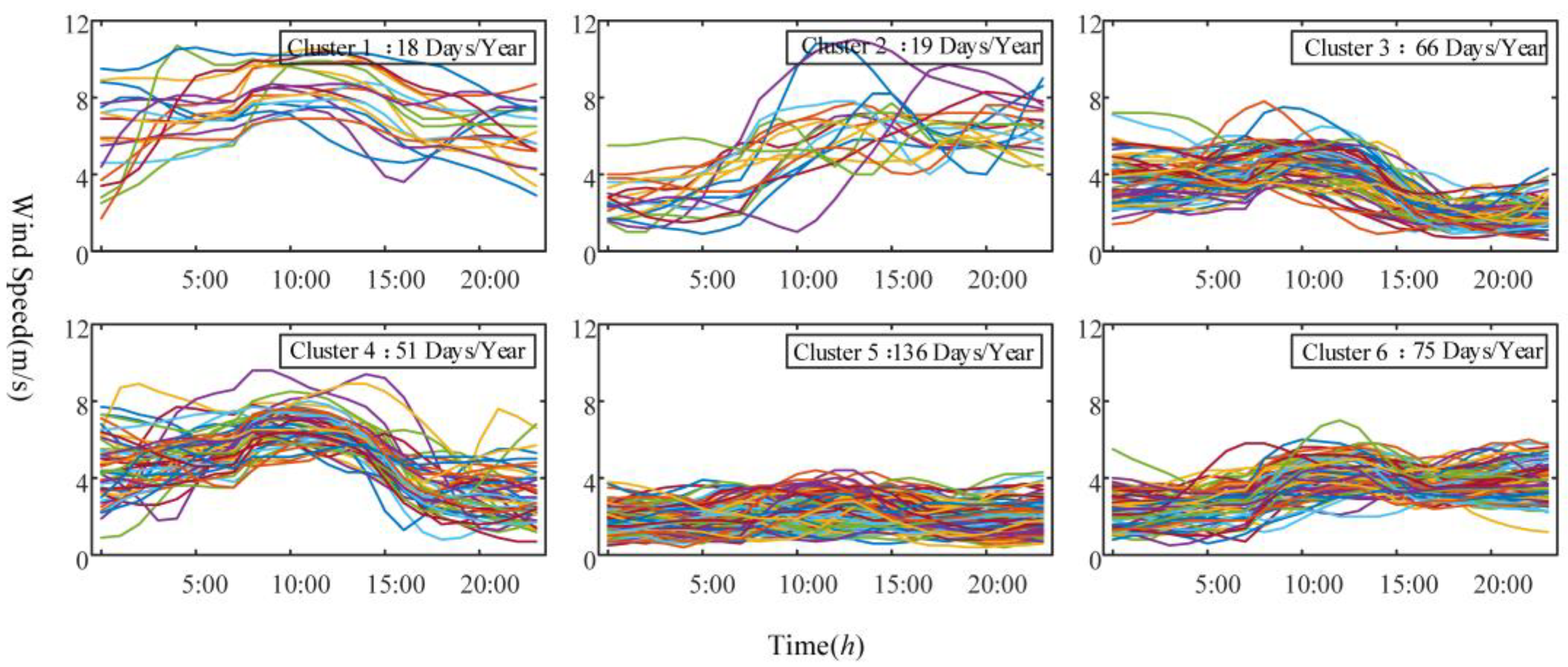
The mean value of all samples is the SC, and the larger the value is, the better the clustering effect is. Figure 3 shows the values of the SC coefficients for the number of clusters from 2 to 20, in which the best clustering is achieved when K = 6. When K = 5, the wind speed of the target power station is clustered, and the wind speed trends of some clusters in the clustering results will be more complicated, thus not having specific characteristics to meet high intra-cluster similarity. In this case, the SC coefficient is 0.14, which is obviously lower than the SC coefficient (0.25) when K = 6. Therefore, the clustering effect is better when the number of clusters is 6. Figure 4 represents the clustering results of the data from 1 January 2014 to 31 December 2014 for the target power station under the optimal number of clusters, while Figure 5 depicts the characteristics of the wind speed data distribution within each cluster through a box line plot of the target power station. Similarly, Figure 6 and Figure 7 show the analysis results of the source power stations. The solid blue lines refer to the clustering centers under each cluster.
In Figure 4, Figure 5, Figure 6 and Figure 7, the horizontal coordinate represents the time with a resolution of 1 h and the vertical coordinate is the wind speed. From Figure 4 and Figure 6, it can be seen that the distribution characteristics of the clustering results of the two power stations are extremely similar, while the distribution of each cluster has its own unique characteristics. Figure 5 and Figure 7 indicate that the clustering centers of each cluster are able to envelop within the box line diagram and are able to match the trend of wind speed for each day. Among them, Cluster 1 has a high overall wind speed level with a large peak wind speed and a large range of wind speed fluctuations, which shows an overall accelerated upward trend from 7:00 to 16:00 as well as an upward followed by downward trend with a significantly higher wind speed at noon than at night. Cluster 2 shows a continuous upward trend, with less fluctuation in wind speed and more outliers. Cluster 3 shows the opposite trend to Cluster 2, that is, a general downward trend from 0:00, with a slightly lower overall wind speed level than Cluster 2 in only few scenarios. Cluster 4 has a similar trend to Cluster 1 with a relatively greater horizontal fluctuation and a much smaller vertical fluctuation range, showing that the wind speed is greater at noon than at night, and there are more outlier points. Cluster 5 has a smooth wind speed variation and a lowest overall wind speed level with a maximum value of 4.4 m/s, but the cluster has the largest number of scenario days at 136, which shows that the wind speed level in the region is generally low and varies steadily. Cluster 6 has a similar trend to Cluster 2 with relatively much less volatility and overall level of wind speed. The unique differential distribution among clusters proves that the clustering results can effectively reflect the wind speed distribution characteristics of the region, and that there are strong similarities between source and target power plants.

3.2. RAC-GAN-Based Wind Power Output Scenario Generation

3.2.1. Aided Classification Generates Adversarial Networks

Generative adversarial networks (GAN) are deep learning models that contain two parts: a generator (G) and a discriminator (D). In the scenario generation model, the purpose of G is to generate data as close as possible to the real sample distribution by learning the distribution characteristics of the wind power output data distribution, and the purpose of D is to maximize the difference between the sample generated by G and the real sample x . The two play a two-person zero-sum game and finally reach a Nash equilibrium state [16].
Specifically, the historical scenario data is defined as real data. For the G network, a set of random noise data z is defined as the input to the generator, and the probability distribution of z is denoted by P Z while the real distribution of historical data is denoted by P X . The output of G is the learned generated data sample G ( z ) with probability distribution P G . Thus, the training objective of G is to make P G as identical to P X as possible [17].
For the D network, its input is the real data x or the data G ( z ) generated by G. The output is a scalar D ( G ( z ) ) , which represents the probability that the input data samples obey P X . The training goal of the discriminator is to discriminate the correctness of the input data compared to the real data.
According to the training objectives of the generator and the discriminator, the loss functions L G and L D of the generator and the discriminator are constructed, respectively, as follows:
L G = E z p z ( z ) [ l o g ( 1 D ( G ( z ) ) ) ]
L D = E x p dat   ( x ) [ l o g D ( x ) ] + E z p z ( z ) [ l o g ( 1 D ( G ( z ) ) ) ]
The optimization objective of the generator is to minimize Equation (10), and the objective of the discriminator is to maximize Equation (11). Combining Equations (10) and (11), the objective function in the GAN training process is obtained as follows:
m i n G m a x D V ( D , G ) = E x p dat ( x ) [ l o g D ( x ) ] + E z p s ( z ) [ l o g ( 1 D ( G ( z ) ) ) ]
In this function, E (·) represents the expected value.
The auxiliary classifier generative adversarial network (AC-GAN) can add random noise signal labeling and multi-classification function to the generative adversarial network and can generate samples of specified types according to the labels [18]. By adding the random noise signal z and the corresponding label c of the generated samples to the generator G of AC-GAN, the generator purposely generates the corresponding category samples X fake = G ( c , z ) . The samples X output by the discriminator D are derived from the real samples X r e a l and the probability P ( S X ) of the generated samples X fake as well as the probability P ( C X ) of belonging to different categories, i.e.,
D ( X ) = ( P ( S X ) , P ( C X ) )
In this equation, P ( · ) is the probability function; S is the source of the sample, which has two possibilities (real (real) and generated (fake)). C = c . Where c { 1 , 2 , , M } , M is the number of sample classes. In AC-GAN, the objective function of G is to maximize L C L S , and the objective function of D is to maximize L C + L S . The expressions of L S and L C are, respectively, as follows:
L S = E l o g P S = r e a l X real + E l o g P S = f a k e X fake L C = E l o g P C = c X real + E l o g P C = c X fake
In the equation, E ( · ) is the Expectation function; L S is the correct source loss function, which can discriminate the correctness of the data source; L C is the correct class loss function, which can discriminate the correctness of the output class. Through the internal game between the generator and the discriminator, the generator is alternately optimized in the iterative process, and the scenario generation capability of the generator is finally improved.
In order to meet the need for multi-label wind power scenario generation, firstly, the data encoder is introduced to the generator input of AC-GAN, thus making its model pre-learn the shallow raw data features based on the real wind power output and its characteristic data to obtain the random noise input [19] instead of directly using random noise signal. Then, the signal is input to the generator so that it can generate a large amount of target-oriented data that meet the real sample probability distribution characteristics. After that, the generated samples, together with the original samples, are input to the discriminator to discriminate their quality, thus expanding the training sample data. During the iteration of the RAC-GAN model, the game optimization is carried out under the principle of reducing the noise impact, so robust scenario generation with multiple labels under noise interference is realized.

3.2.2. RAC-GAN-Based Wind Power Output Scenario Generation

There are different scenario characteristics among each day in the original data set of the source power plant. To improve the effectiveness of wind power output scenario generation, wind speed is clustered to obtain multiple cluster labels and assign labels to each scenario in the original data set to achieve targeted scenario generation in the corresponding cluster labels. The RAC-GAN model is proposed in a complex scenario where no historical output data are available for newly built power plants, and the target power plant output scenarios need to be generated with the assistance of source power plant output data, i.e., the scenarios with noise, as shown in Figure 8. In the Figure 8, DP denotes the dropout layer, TC denotes the deconvolution layer, and FC denotes the fully connected layer [19].
Based on the above RAC-GAN scenario generation model, a large number of wind power output scenarios are generated by the K-means clustering method, in which 365 historical samples are input, each containing 24 h of power output data in a day.

4. Evaluation of Scenario Generation Effects

The evaluation of scenario generation effects requires an analysis of the probability distribution characteristics of the scenarios. Therefore, the following characteristics should be considered to judge the quality of scenarios generated with the method proposed in this paper:
  • the power output data of the selected source power station should be similar to that of the target power station (no power output data of the target power station are assumed during the experiment, but they should be analyzed during the evaluation);
  • the probability distribution of scenarios generated by the power output data of the source power station should be similar to that of the target power station;
  • the method proposed in this paper should be more advantageous when compared with other existing deep learning-based scenario generation methods.
Accordingly, this paper firstly compares the similarity of the probability density function and cumulative probability distribution of the proposed method and verifies (1) and (2) above, and the comparison subjects contain the probability density function and cumulative probability distribution of the output data of the source power station, the output data of the target power station, and the output data of the generated scenes. Then, a variety of comparative experiments are set up to analyze the superiority of the proposed method compared with other methods, during which the evaluation indicators such as probability distribution characteristics are used.

4.1. Characterization of Probability Distributions

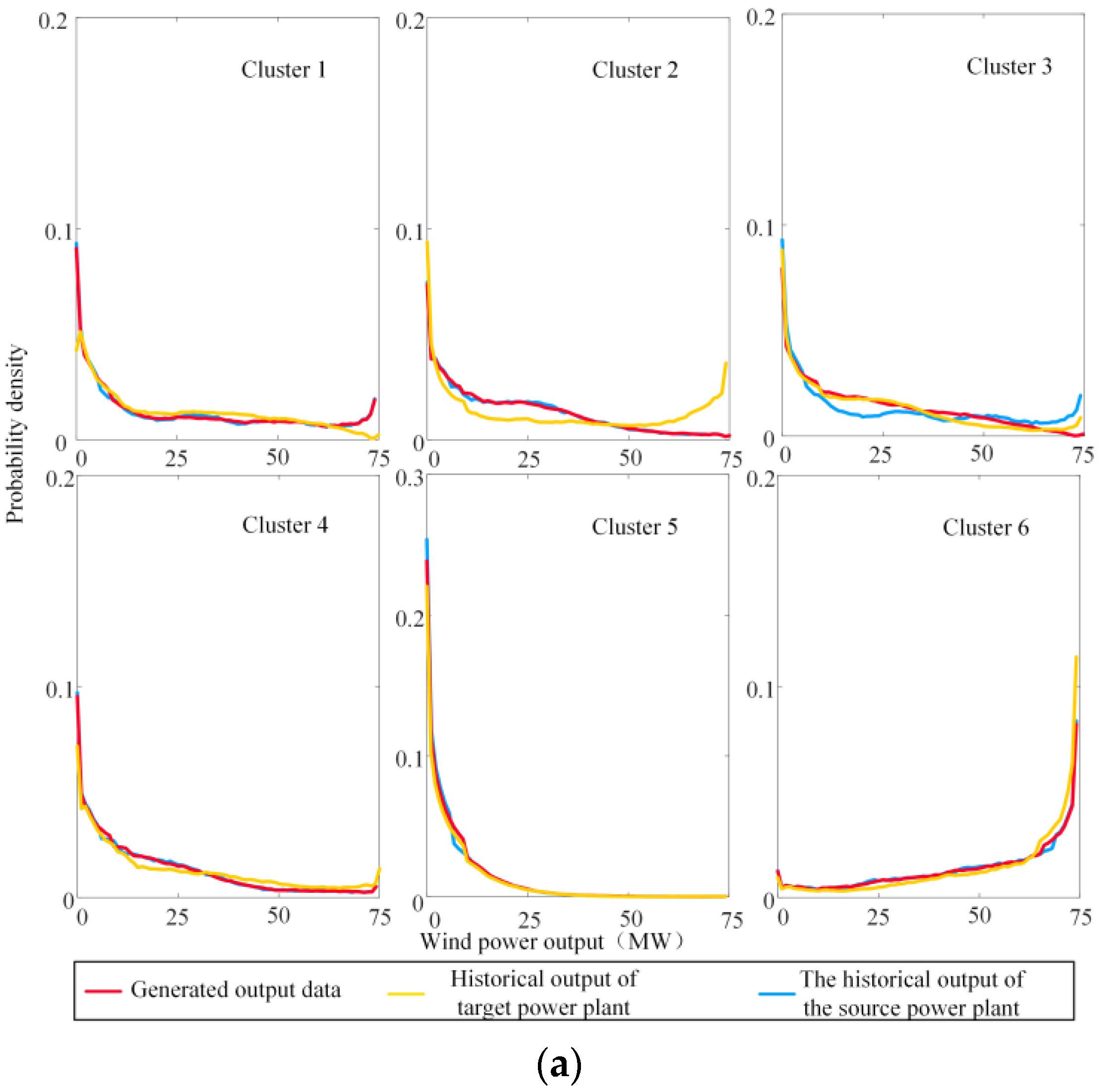
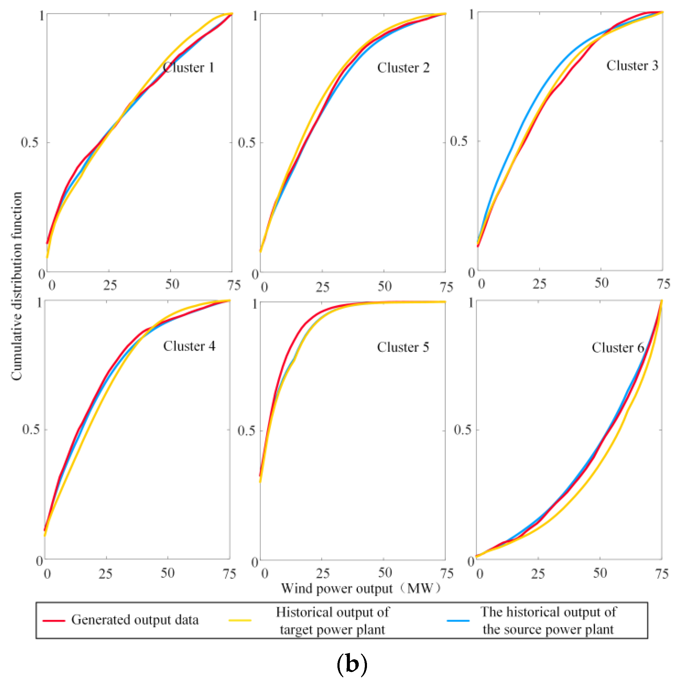
The probability density functions and cumulative probability distributions of the source power plant output data, the target power plant output data, and the output data of the generated scenarios are experimented, and the results are shown as Figure 9a,b below. In Figure 9, the horizontal coordinate represents the wind power output with a maximum value of 75 MW, and the vertical coordinate is the probability distribution and cumulative probability distribution. Since the probability of low output in Cluster 5 in Figure 9a is too large, the maximum value of the vertical coordinate in Cluster 5 is 0.3 and the maximum value of the vertical coordinate in other clusters is set to 0.2 for the convenience.
In Figure 9a,b, it can be seen that the probability density distribution and cumulative probability distribution between the generated wind power output data of each cluster and the source power station are very close, which demonstrates the effectiveness of the proposed scenario generation method in this paper. In Cluster 2, there is a difference in the probability density of the high wind power output part, and the historical output of the target plant has a higher probability in the high wind power output part, while the generated output probability is lower; in Cluster 1, there is a gap between the probability of the target plant and the generated data when approaching 75 MW, and the target plant has a lower probability of high output; on the contrary, the level of probability of high output is higher in the target plant in Cluster 6. In terms of source power plant output scenarios and generation scenarios, the above three differences have good fitting performances. The reason for this is that the scenario generation method proposed in this paper is based on the data of the source power plant, which are well fitted to the source power plant, while there is a difference in the output distribution between the source power plant and the target power plant in Cluster 2. In general, the scenario generation method proposed in this paper is able to generate scenarios for newly built wind farms well, in spite of minor differences.

4.2. Comparison of Methods of Scenario Generation

In order to demonstrate the superiority of the proposed scene generation method, the new method is compared with the existing scenario generation methods based on a deep learning framework and other methods to determine the source power station, and several comparison experiments are set up. Model 1 is the proposed scenario generation method. Model 2 uses the clustering results as cluster labels, and the C-GAN method is used for scenario generation. Model 3 selects the source power station by geographical location and uses the RAC-GAN method for scenario generation. Model 4 selects the source power station by altitude and uses the RAC-GAN method for scenario generation.

4.2.1. Properties of the Probability Distribution of the Comparison Experiment

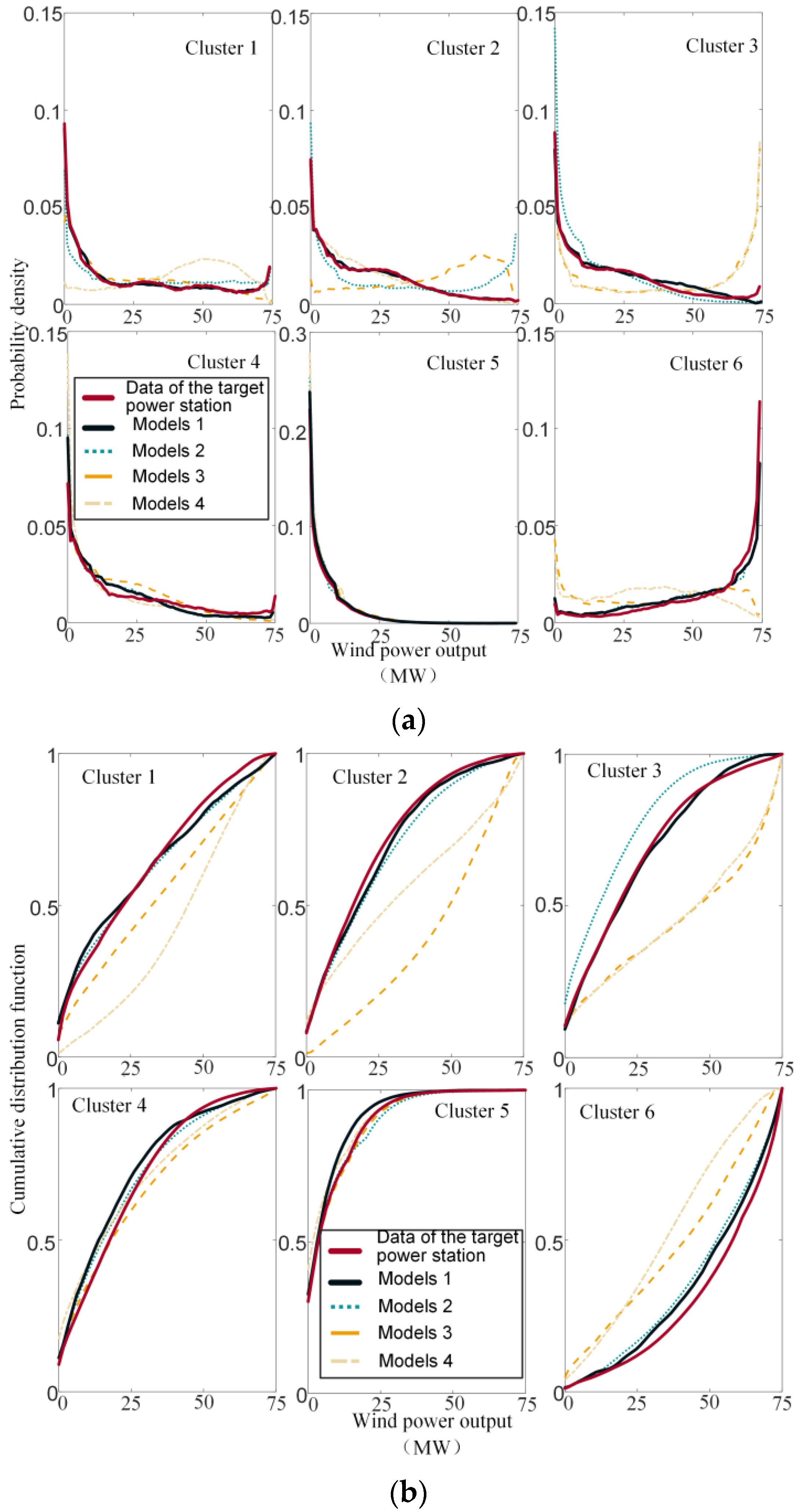
The probability density function curves and cumulative probability distribution curves for each model are shown below in Figure 10a,b. Similar to Figure 9, the maximum value of the vertical coordinate in Figure 10a is 0.15 except for Cluster 5, and the maximum value of the vertical coordinate in Cluster 5 is 0.3.
The following results can be seen from Figure 10:
  • From the comparison of Model 1 and Model 2, it can be seen that the difference between Model 1 and Model 2 is small in Clusters 3 to 6 in terms of probability distribution characteristics. Model 1 is slightly better than Model 2, and the generated data fit the real data better. From the probability distribution characteristics of Cluster 1 and Cluster 2, it can be seen that both Model 1 and Model 2 are more effective when Cluster 1 is near 25 MW and Cluster 2 is near 45 MW, except for these two places, where Model 1 is much stronger than Model 2 overall. Combined with Figure 4 and Figure 6, it can be seen that both Cluster 1 and Cluster 2 are characterized by a small number of scenes, only 18 and 19 days, respectively, i.e., the number of historical data is small, while Model 2 uses the C-GAN method for scene generation, which is not effective in generating scenes with little historical data. Therefore, the proposed method in this paper can achieve a better fitting effect when there are less data.
  • Comparing Model 1 with Model 3 and Model 4, it can be seen that Model 1 is significantly better than Model 3 and Model 4 in scenario generation for each cluster. This is because the method used in this paper for the selection of source power stations can analyze whether the time-series wind speed data are consistent in terms of change trends, and the selection of source power plants is based on the changing characteristics of wind speed data, while Model 3 and Model 4 are based on geographical factors in the selection of original power plants, which are similar in terms of geographical location or altitude, but cannot reflect the characteristics of wind speed data, which is the most critical factor for wind power output. Therefore, the generated data do not fit the historical data well in terms of probability distribution characteristics. Meanwhile, under the premise that both RAC-GANs are used for scene generation, the scenes generated by using Model 3 and Model 4 to select source power plants have poor performance in each cluster, which can indicate that the appropriate selection of source power plants is an important factor.

4.2.2. Evaluation of Scenario Generation Effects

In order to furtherly compare the wind power output scenario generation effects of the model proposed in this paper with that of each model in comparative experiments, the Root Mean Squared Error (RMSE), the Mean Absolute Error (MAE), and the coefficient of determination R 2 are selected in this paper. RMSE, MAE, and R 2 are defined as follows [20,21,22].
R M S E = 1 T t = 1 T x ^ t x t 2
M A E = 1 T t = 1 T x ^ t x t
R 2 = t = 1 T x ^ t x 2 t = 1 T x t x 2
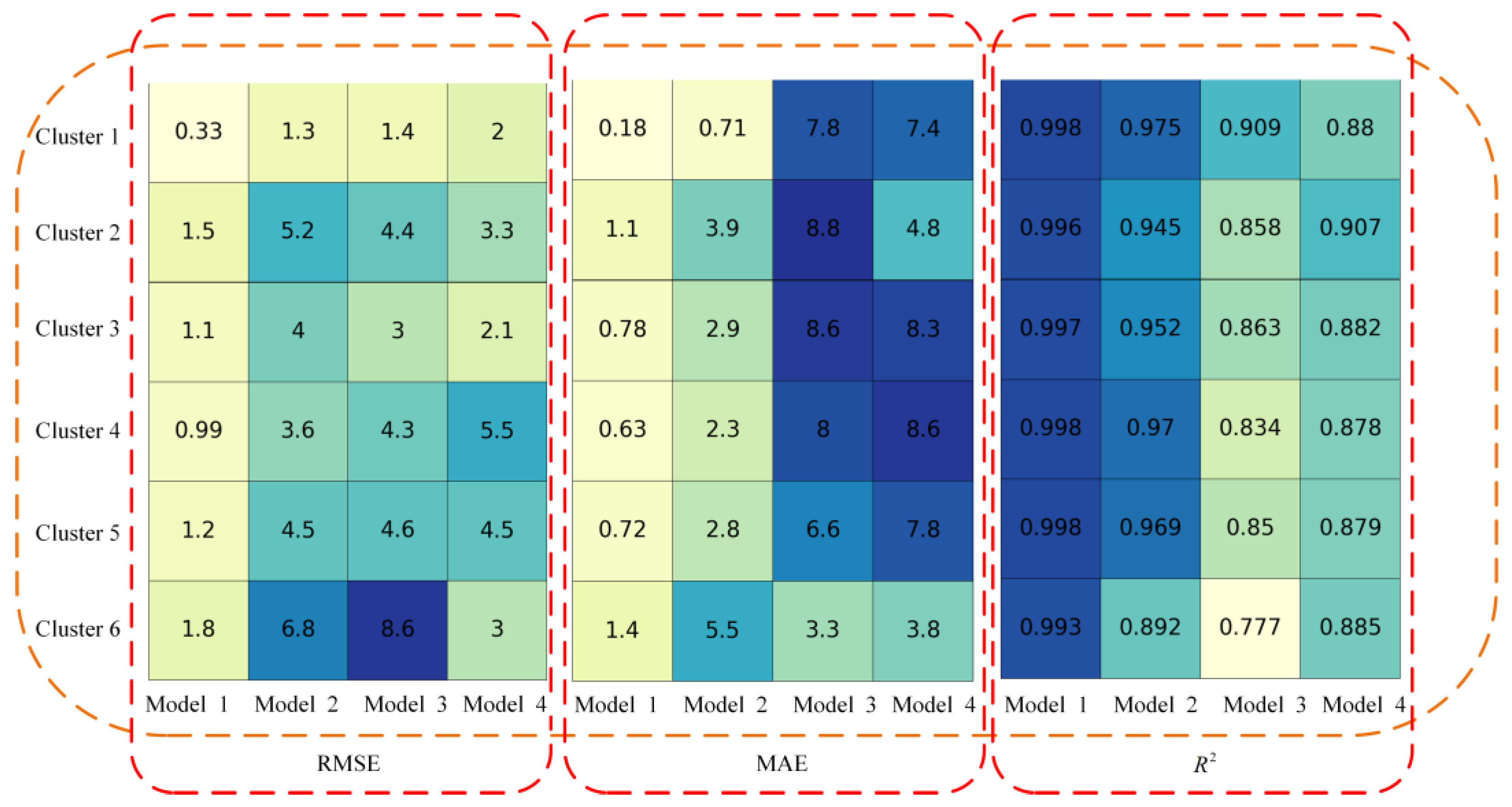
In the equation above, T denotes the total number of generated scene data; x ^ t , x t and x denote the average of generated scenario value sampling points, real scene value sampling points, and real scene data, respectively. The RMSE and MAE are used to evaluate the error between the generated scene data and the real scenario data. The smaller the error is, the closer the generated data are to the real data. The closer R 2 is to 1, the more the generated scene data can correctly represent the real scenario data. The scenario data generated by each model are tested by each statistical index, and the test results are shown in Figure 11 below.
It is notable in Figure 11 that,
  • From the comparison of Model 1 and Model 2, it can be seen that the RMSE in Model 1 is smaller with the average value of 1.153 and the maximum value of 1.8, which is much lower than Model 2 (the average value is 4.23 and the maximum value is 6.8); similarly, the MAE in Model 1 (the average value is 0.801 and the maximum value is 1.4) is much smaller than that of Model 2 (the average value is 3.02). Therefore, the scene generation using RAC-GAN has good results.
  • The comparison between Model 1, Model 3, and Model 4 shows that the three evaluation indexes of Model 1 outperform those of Model 3 and Model 4. Moreover, the generation results of Model 2 are stronger than those of Model 3 and Model 4, which indicates that the selection method of source power plants is important for scene generation results. The selection of source power plants by using the GRA method is more effective than that of using geographical factors.
Each evaluation index of Model 1 can numerically show that the proposed scenario generation method as well as source power plant selection method has a good performance in new wind farm scenario generation.

5. Conclusions

This paper constructs a RAC-GAN-based scenario generation method for new wind farms, which is the first of its kind in terms of meteorological factors selection, source power plant selection for scenario generation, and scenario generation with labeling, in response to the problem that there are few power data for new wind farms and it is difficult to study the planning and scheduling of power farms. The proposed scenario generation method can better realize the scenario generation of new wind farms, effectively filling the data gap of new wind farms.
The paper uses the Pearson correlation coefficient to filter the meteorological factors affecting wind power output, where wind speed is the most critical factor and the correlation coefficient between them is 0.8, indicating a very high correlation. GRA is used to select the source power station, and the source power station is selected based on the principle of consistency of the change trend of time series data. In the scenario generation part, based on the historical output data of source power plants, the K-means clustering method is used to cluster the wind power output, and the cluster information of the clustering result is used as a label to generate the wind power output scenario of new wind farms by the RAC-GAN method. The proposed method performs better with each evaluation index, and the values of RMSE, MAE, and R 2 are significantly better than in other scenario generation methods and source plant selection methods; thus, the probability distribution characteristics are closer to the target plant.
The limitations of this paper are mainly reflected in that when analyzing the consistency of meteorological data between source and target power stations, the time-shifted characteristics of the data due to geographical location are not taken into account, i.e., the data consistency between two power stations is stronger at a certain time interval, which will lead to the same characteristics of wind power output. Therefore, the length of the time interval and its influencing factors should be focused on the analysis of the consistency of the wind speed and wind power output time series data trends in the future, which will have a positive impact on the scenario generation effect. In addition, subsequent studies will use shorter time scales (30 min, 15 min, or 5 min) of data for scenario generation and analyze scenario generation methods with larger data volumes.

Author Contributions

J.T.: Conceptualization, Data curation; J.L.: Formal analysis, Investigation; J.W.: Supervision, Methodology; G.J.: Investigation, Software; H.K.: Validation, Visualization; Z.Z.: Writing—review & editing, Resources; N.H.: Funding acquisition, Writing—original draft, Project administration. All authors have read and agreed to the published version of the manuscript.

Funding

This research was funded by Economic and Technological Research Institute of State Grid Inner Mongolia Eastern Power Co., Ltd. and National key R & D plan, grant number “SGTYHT/21 JS-223” and “2019YFB1505405”.

Data Availability Statement

Not applicable.

Conflicts of Interest

The company of the five authors (J.T., J.L., G.J., H.K. and Z.Z.), provide technical and financial support for this paper. (Economic and Technological Research Institute of State Grid Inner Mongolia Eastern Power Co., Ltd.: SGTYHT/21-JS-223).

Nomenclature

RCorrelation coefficient of two variables.
c o v ( X , Y ) Covariance of the two variables.
σ X ,   σ Y Standard deviation of X and Y .
X ,   Y Average of X and Y .
F g i Wind speed at the g t h moment of the i t h day.
F a v i Average wind speed on the i t h day.
x ,   x m i n ,   x m a x Arbitrary values, minimum values and maximum values in the original data.
x Normalized data.
x 0 i Eigenvector of the target power station on day i .
x j i Eigenvector of the j t h historical day of the i t h proximity power station.
x 0 i ( n ) ,   x j i ( n ) n t h element of the j t h historical day feature vector of the target power station, the i t h proximity power station.
ξ i ( n ) Number of correlation coefficients.
r Resolution factor.
N Total number of correlation coefficients for each component.
v , v r ,   v in ,   v out Wind speed, the rated wind speed, the cut-in and cut-out wind speed.
P W T Rated power of the fan.
m Number of clustered samples.
k Number of clusters.
b ( k ) Minimum   average   distance   of   sample   k to the samples of other clusters.
a ( k ) Average   distance   of   sample   k to other samples in the same cluster.
G ( z ) , D ( G ( z ) ) Output ofs G and D network in GAN.
E (·)Expected value.
L S ,   L C Correct source loss function and class loss function.
x ^ a ,   x a ,   x Average of generated scene value sampling points, real scene value sampling points, and real scene data.

References

  1. Hu, J.X.; Li, H.R. A transfer learning-based scenario generation method for stochastic optimal scheduling of microgrid with newly-built wind farm. Renew. Energy 2022, 185, 1139–1151. [Google Scholar] [CrossRef]
  2. Tu, Q.Y.; Miao, S.H.; Yao, F.X.; Li, Y.W.; Yin, H.R.; Han, J.; Zhang, D.; Yang, W.C. Forecasting Scenario Generation for Multiple Wind Farms Considering Time-series Characteristics and Spatial-temporal Correlation. J. Mod. Power Syst. Clean Energy 2021, 9, 837–848. [Google Scholar] [CrossRef]
  3. Tan, J.; Wu, Q.W.; Zhang, M.L.; Wei, W.; Hatziargyriou, N.; Liu, F.; Konstantinou, T. Wind power scenario generation with non-separable spatio-temporal covariance function and fluctuation-based clustering. Int. J. Electr. Power Energy Syst. 2021, 130, 106955. [Google Scholar] [CrossRef]
  4. Zhang, R.; Li, G.; Bu, S.; Kuang, G.; He, W.; Zhu, Y.; Aziz, S. A Hybrid Deep Learning Model with Error Correction for Photovoltaic Power Forecasting. Front. Energy Res. 2022, 10, 1103. [Google Scholar] [CrossRef]
  5. Zhang, Y.F.; Ai, Q.; Xiao, F.; Hao, R.; Lu, T.G. Typical wind power scenario generation for multiple wind farms using conditional improved Wasserstein generative adversarial network. Int. J. Electr. Power Energy Syst. 2020, 114, 105388. [Google Scholar] [CrossRef]
  6. Cramer, E.; Paeleke, L.; Mitsos, A.; Dahmen, M. Normalizing flow-based day-ahead wind power scenario generation for profitable and reliable delivery commitments by wind farm operators. Comput. Chem. Eng. 2022, 166, 107923. [Google Scholar] [CrossRef]
  7. Wang, K.S.; Yu, H.; Song, G.Y.; Xu, J.; Li, J.; Li, P. Adaptive forecasting of diverse electrical and heating loads in community integrated energy system based on deep transfer learning. Front. Energy Res. 2022, 10, 8216. [Google Scholar] [CrossRef]
  8. Chen, Y.Z.; Wang, Y.S.; Kirschen, D.; Zhang, B.S. Model-Free Renewable Scenario Generation Using Generative Adversarial Networks. IEEE Trans. Power Syst. 2018, 33, 3265–3275. [Google Scholar] [CrossRef] [Green Version]
  9. Tang, C.H.; Wang, Y.S.; Xu, J.; Sun, Y.Z.; Zhang, B.S. Efficient scenario generation of multiple renewable power plants considering spatial and temporal correlations. Appl. Energy 2018, 221, 348–357. [Google Scholar] [CrossRef]
  10. Huang, N.T.; He, Q.K.; Qi, J.J.; Hu, Q.K.; Wang, R.J.; Cai, G.W.; Yang, D.Z. Multinodes interval electric vehicle day-ahead charging load forecasting based on joint adversarial generation. Int. J. Electr. Power Energy Syst. 2022, 143, 108404. [Google Scholar] [CrossRef]
  11. Feng, Z.-k.; Niu, W.-j.; Zhang, R.; Wang, S.; Cheng, C.-t. Operation rule derivation of hydropower reservoir by k-means clustering method and extreme learning machine based on particle swarm optimization. J. Hydrol. 2019, 576, 229–238. [Google Scholar] [CrossRef]
  12. Fan, Y.; Liu, C.; Wang, J. Prediction algorithm for springback of frame-rib parts in rubber forming process by incorporating Sobol within improved grey relation analysis. J. Mater. Res. Technol. 2021, 13, 1955–1966. [Google Scholar] [CrossRef]
  13. Zolfani, S.H.; Gorcun, O.F.; Kundu, P.; Kucukonder, H. Container vessel selection for maritime shipping companies by using an extended version of the Grey Relation Analysis (GRA) with the help of Type-2 neutrosophic fuzzy sets (T2NFN). Comput. Ind. Eng. 2022, 171, 108376. [Google Scholar] [CrossRef]
  14. Lee, C.; Lee, J.W.; Ryu, S.G.; Oh, J.H. Optimum design of a large area, flexure based XY theta mask alignment stage for a 12-inch wafer using grey relation analysis. Rob. Comput. Integr. Manuf. 2019, 58, 109–119. [Google Scholar] [CrossRef]
  15. Huang, N.; Wang, W.; Cai, G. Optimal configuration planning of multi-energy microgird based on deep joint generation of source-load-temperature scenarios. CSEE J. Power Energy Syst. 2020. [Google Scholar] [CrossRef]
  16. Xu, J.; Li, H.; Hou, S. Autoencoder-guided GAN for minority-class cloth-changing gait data generation. Digit. Signal Process. 2022, 128, 103608. [Google Scholar] [CrossRef]
  17. Zhu, B.; Pan, X.; vanden Broucke, S.; Xiao, J. A GAN-based hybrid sampling method for imbalanced customer classification. Inf. Sci. 2022, 609, 1397–1411. [Google Scholar] [CrossRef]
  18. Dharanya, V.; Raj, A.N.J.; Gopi, V.P. Facial Expression Recognition through person-wise regeneration of expressions using Auxiliary Classifier Generative Adversarial Network (AC-GAN) based model. J. Visual Commun. Image Represent. 2021, 77, 103110. [Google Scholar] [CrossRef]
  19. Huang, N.; Chen, Q.; Cai, G.; Xu, D.; Zhang, L.; Zhao, W. Fault Diagnosis of Bearing in Wind Turbine Gearbox under Actual Operating Conditions Driven by Limited Data with Noise Labels. IEEE Trans. Instrum. Meas. 2021, 70, 1–10. [Google Scholar] [CrossRef]
  20. Yang, R.; Yang, X.; Wang, L.; Li, D.; Guo, Y.; Li, Y.; Guan, Y.; Wu, X.; Xu, S.; Zhang, S.; et al. Commissioning and clinical implementation of an Autoencoder based Classification-Regression model for VMAT patient-specific QA in a multi-institution scenario. Radiother. Oncol. 2021, 161, 230–240. [Google Scholar] [CrossRef]
  21. Ren, F.; Long, D. Carbon emission forecasting and scenario analysis in Guangdong Province based on optimized Fast Learning Network. J. Clean. Prod. 2021, 317, 128408. [Google Scholar] [CrossRef]
  22. Wang, Y.; Shen, R.; Ma, M. Research on ultra-short term forecasting technology of wind power output based on various meteorological factors. Energy Rep. 2022, 8, 1145–1158. [Google Scholar] [CrossRef]
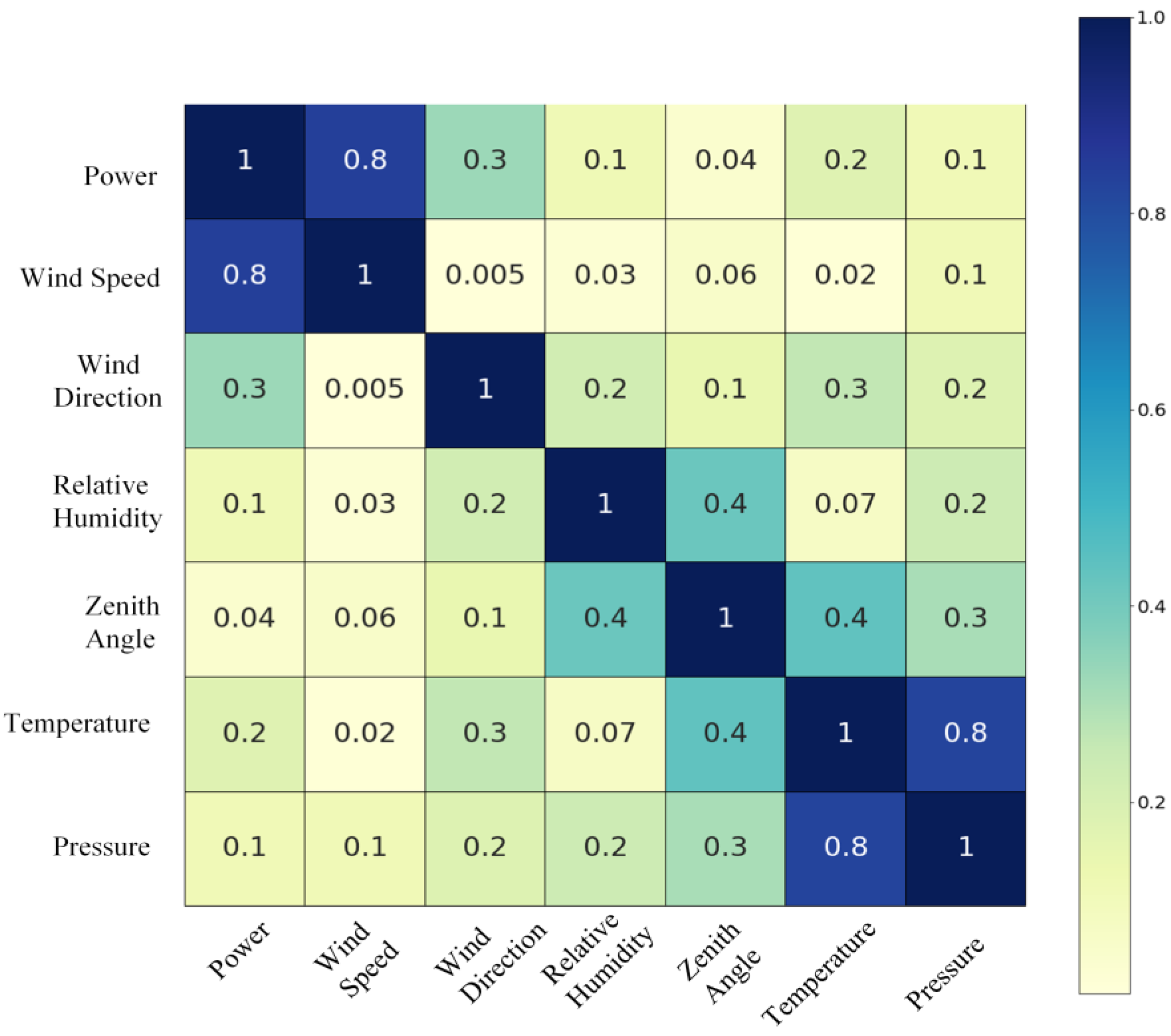
Figure 1. Pearson coefficient meteorological correlation analysis.
Energies 16 02447 g001
Figure 2. Correlation analysis of GRA of wind speed in multiple wind farms.
Energies 16 02447 g002
Figure 3. SC values at each number of clusters for wind speed data from source power plants.
Energies 16 02447 g003
Figure 4. Wind speed scenarios within each cluster of the target power plants.
Energies 16 02447 g004
Figure 5. Wind speed clustering results of target power stations.
Energies 16 02447 g005
Figure 6. Wind speed scenarios in each cluster of the source power plant.
Energies 16 02447 g006
Figure 7. Source power station wind speed clustering results.
Energies 16 02447 g007
Figure 8. Model structure of improved RAC-GAN.
Energies 16 02447 g008
Figure 9. Comparison of the data probability distribution characteristics of the generated scenes of each cluster source power plant and the real scenes of the target power plant. (a) Probability density function. (b) Cumulative distribution function.
Energies 16 02447 g009aEnergies 16 02447 g009b
Figure 10. Results of probability distribution characteristics of each Model. (a) Probability density function curve of each Model. (b) Cumulative probability distribution curves for each Model.
Energies 16 02447 g010
Figure 11. Evaluation results of each Model generation scenario evaluation index.
Energies 16 02447 g011
Table 1. Criteria for judging the strength of relevance.
Absolute Value of Correlation CoefficientStrength of Correlation
[0.8, 1.0]Extremely strong correlation
[0.6, 0.8]Strong correlation
[0.4, 0.6]Moderate correlation
[0.2, 0.4]Weak correlation
[0, 0.2]Very weak or no correlation
Table 2. Wind farm latitude and longitude information.
Power StationLatitude (°N)Longitude (°W)
Newly built wind farm39.70121.66
Wind Farm 239.78121.56
Wind Farm 340.02121.82
Wind Farm 442.01121.84
Wind Farm 539.84121.66
Wind Farm 639.54121.57
Disclaimer/Publisher’s Note: The statements, opinions and data contained in all publications are solely those of the individual author(s) and contributor(s) and not of MDPI and/or the editor(s). MDPI and/or the editor(s) disclaim responsibility for any injury to people or property resulting from any ideas, methods, instructions or products referred to in the content.