Article

Design of an Algorithm for Modeling Multiple Thermal Zones Using a Lumped-Parameter Model

by
Pedro Fernández de Córdoba
1,
Frank Florez Montes
2,*,
Miguel E. Iglesias Martínez
1,
Jose Guerra Carmenate
1,
Romeo Selvas
3 and
John Taborda
4
1
Instituto Universitario de Matemática Pura y Aplicada, Universitat Politècnica de València, Camino de Vera s/n, 46022 Valencia, Spain
2
Faculty of Engineering, Universidad Autónoma de Manizales, Manizales 170003, Colombia
3
Facultad de Ciencias Físico-Matemáticas, Universidad Autónoma de Nuevo León, FCFM Av. Universidad S/N, Cd. Universitaria, San Nicolas de los Garza 66455, Nuevo León, Mexico
4
Faculty of Engineering, Universidad del Magdalena, Santa Marta 470003, Colombia
*
Author to whom correspondence should be addressed.
Energies 2023, 16(5), 2247; https://doi.org/10.3390/en16052247
Submission received: 28 January 2023 / Revised: 18 February 2023 / Accepted: 25 February 2023 / Published: 26 February 2023

Abstract

:
The generation of mathematical models for the analysis of buildings with multiple thermal zones is a large and complex task. Furthermore, the order and complexity of the dynamical model are increased by the number of included thermal zones. To overcome this problem, this paper presents an algorithm to define the mathematical model automatically, using the geometric and physics parameters as inputs. Additionally, the spatial position of each thermal zone must be recorded in an arrangement called a contact matrix. The algorithm for modeling systems with multiple thermal zones is the main contribution of this work. This algorithm is presented in pseudocode format and as an annex, an implementation in MATLAB software. One of the advantages of this methodology is that it allows us to work with parallelepipeds and not necessarily cubic thermal zones. The algorithm allows us to generate mathematical models with symbolic variables, starting from the knowledge of how many thermal zones compose the system and its geometric organization. This information must be organized in a matrix arrangement called a contact matrix. Different arrays of thermal zones were constructed with wooden boxes to verify the functionality of the models generated with the algorithm. Each case provided information that allowed us to adjust the mathematical models and their simulations, obtaining a range of errors between experimental and simulated temperatures from 2.08 to 5.6 , depending on the number of thermal zones studied.

1. Introduction

Building modeling is an increasingly important field of research. In the last decade, several papers have been published in this field [1,2,3,4]. This increase has been driven in part by international agreements for environmental protection, such as the Kyoto Protocol [5] and the Paris Agreement [6]. Countries participating in this agreement have committed to formalizing various policies to reduce energy consumption and CO2 emissions, especially in cities and buildings, which, according to additional research, can consume up to 40 % of the annual energy production [7,8,9].
The energy consumption in buildings depends on different factors, such as occupant activity [9] and heating, ventilation and air conditioning (HVAC) systems [10], among others. However, to understand the causes of energy consumption, buildings must be studied individually, taking into account the minimum spaces and energy requirements to ensure occupant comfort [11,12]. In this sense, mathematical models and simulators play an essential role, allowing researchers to analyze different configurations and situations in buildings, including huge interior spaces in buildings [13] or green roofs [14].
Regarding tools and strategies to generate and study the mathematical models of buildings, several works have been carried out [15,16,17,18]. Many works use specific simulators such as Energy Plus [19], Contam [20] and Trnsys [21] to understand and model problems such as choosing the best cooling system, airflow and energy savings [4,10,11]. These issues are considerably more complex if the building has multiple thermal zones. Papers such as in [22,23] mention the use of machine learning strategies to tackle these problems.
In different investigations, the lumped-parameter technique (LPM) is used to analyze thermal zones [7,13]. This technique allows a deeper numerical understanding of the thermal behavior in a closed enclosure, as it allows the user to generate a clear mathematical model, where each term can be explained and studied individually. These models are known as gray-box models and are the equivalent of the black-box models used by academic simulators that do not clearly show the mathematical model used for the simulation [24,25,26].
The LPM makes it possible to generate an equivalent electrical circuit to analyze a thermal zone and, using Kirchhoff’s laws, to define a mathematical model [27,28,29,30]. The order of the model depends on the number of resistors and capacitors used for each wall. However, the size and model requirements increase with the number of thermal zones studied. The need to consider multiple interacting thermal zones arises when studying more realistic buildings, such as residential houses or apartments [31,32,33,34].
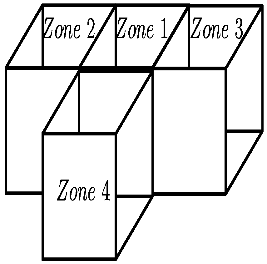
Figure 1 shows different combinations of thermal zones, providing a complex heat- and air-transfer modeling problem. In this paper, an algorithm for modeling multiple thermal zones is presented. The algorithm can be extended to consider as many zones as necessary, requiring only the geometrical and physical parameters and information about the spatial position of each zone. The proposed methodology is not limited to thermal zones having a square geometry. This is a problem presented in similar algorithms [35]. In addition, the algorithm presented in [32] showed a statistical model for multiple thermal zones, but that type of algorithm uses a complex nomenclature and may be more difficult to use than the proposed methodology. Other works presented algorithms for modeling but were limited by the geometry, excessive information requirements and mathematical complexity [15,36,37].
The paper is organized as follows: Section 2 is devoted to describing the different organizations of the thermal zones, classified into cases. The description of the algorithm is given in Section 3. An experimental verification of the different mathematical models is presented in Section 4. Finally, conclusions and future work are presented in Section 6.

2. Mathematical Model

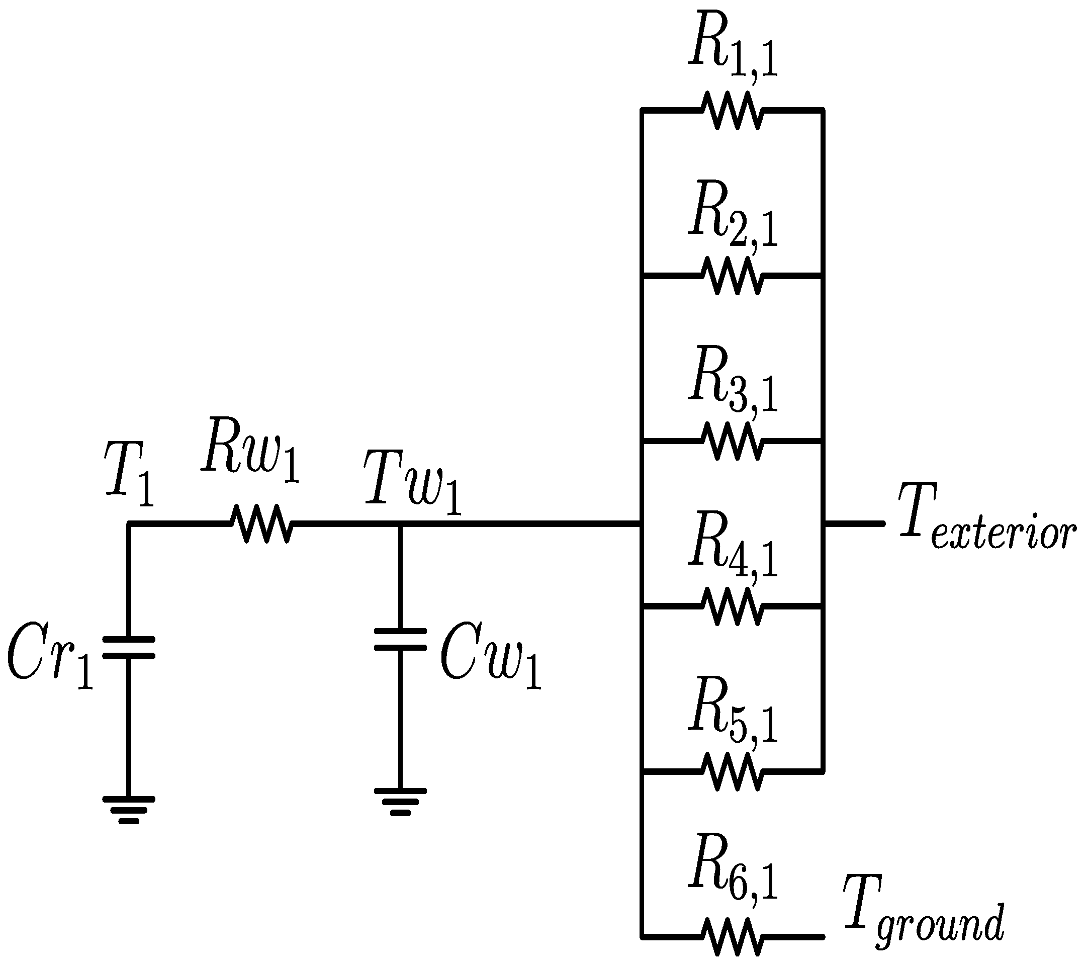
The lumped-parameter technique (LPM) represents the thermal zones with an RC circuit and defines a mathematical model using circuit analysis strategies. The size of the mathematical model can change depending on the structure used. The structure presented in Figure 2 was used in previous work, showing a good behavior and adaptability, and thus was used as equivalent for each thermal zone studied in this work [37,38,39].
The resistance and capacitors are calculated as a function of the geometric and physical parameters of the thermal zones, such as wall dimensions (L for thickness and A for surface area), density ( ρ ), thermal conductivity ( k t ) and specific heat ( C e ). Equations (1)–(6) show the relationships for each surface. The subscripts i and j have a key function: i represents each wall in the thermal zone. Because of that, i = 1 , 2 , , 6 in all the cases. Furthermore, the subscript j represents the number of analyzed thermal zones (m), so j = 1 , 2 , , m .
R i , j = L i , j 2 k t i , j A i , j
R i n j = 1 h i j A i , j
R e x j = 1 h e j A i , j
R w j = k = 1 6 ( R k , j + R i n j ) i = 1 6 k = 1 6 R k , j + R i n j R i , j + R i n j
C w j = i = 1 6 ρ i C e i A i L i
C r j = ρ a C e a V a
The resistance R i , j represents the thermal resistance of the exterior half-wall and can be extended to include heat transfer to the surroundings by adding Equation (2) for cases where the surface is exposed to outside air. The resistance R w j corresponds to the parallel reduction of the resistances of the inner half-walls. The constants h i and h e are the heat transfer coefficients between the walls and the indoor and outdoor air, respectively. These values must be adjusted to each specific environmental situation [40,41]. Finally, C w j and C r j are used to represent the thermal capacity of the walls and internal air, respectively.
Traditionally, the process of developing a mathematical model using LPM consists of three stages:
  • The identification of geometrical and physical parameters of the thermal zones, including internal loads.
  • RC circuit construction and the calculation of resistors and capacitors
  • Define the equations of the dynamic system, using the theory of energy flow transfer.
These three steps can be arduous if the system includes several thermal zones. In addition, this section represents the final two steps of the analysis of a thermal zone with different spaces.

2.1. Case 1: A Single Thermal Zone (m = 1)

To facilitate understanding of the notation, the same wall numbering is always used in the remainder of this paper. Figure 3 shows the chosen assignment, taking the front and back faces as walls one and two, the right and left walls are denoted by walls three and four. Meanwhile, surfaces five and six are the top and bottom surfaces, respectively.
The circuit for the single thermal zone case is presented in Figure 2. Using classical electrical circuit analysis strategies, Equations (7) and (8) were defined, where T w and T represent the wall and indoor-air temperature, respectively.
C w 1 T w 1 ˙ = T 1 R w 1 T w 1 1 R 1 , 1 + 1 R 2 , 1 + 1 R 3 , 1 + 1 R 4 , 1 + 1 R 5 , 1 + 1 R 6 , 1 + 1 R w 1 + 1 R 1 , 1 + 1 R 2 , 1 + 1 R 3 , 1 + 1 R 4 , 1 + 1 R 5 , 1 T e x t e r i o r + T g r o u n d R 6 , 1
C r 1 T 1 ˙ = T 1 R w 1 + T w 1 R w 1
The state variable for this case can be shortened to X = T w 1 T 1 T , the inputs to the system are the ambient temperature denoted by T e x t e r i o r and the ground temperature denoted by T g r o u n d ; for the specific situation where the thermal zone is separated from the ground, the ground temperature must be substituted for the environmental temperature. In addition, Equation (8) can be extended to include thermal loads by adding the term ± Q , taking Q as the power of the load, positive when the load is a heating load, and negative when the load is a cooling system. This case was studied in previous works and was not analyzed in depth in this paper [40,42].

2.2. Case 2: Two Thermal Zones (m = 2)

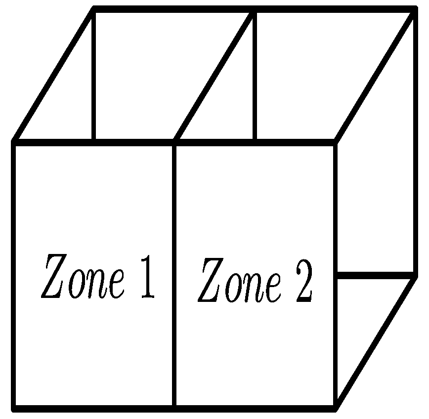
Figure 4 shows the spatial location of the thermal zones. In this configuration, surface 3 of zone 1 is in contact with surface 4 of zone 2, according to the numbering presented in Figure 3.
For the case with two thermal zones, the circuit presented in Figure 2 must be extended to include the second thermal zone; Figure 5 shows the new circuit, taking T w 2 and T 2 as the temperatures for the second zone. Using the circuit for two thermal zones it is possible to derive Equations (9) to (12).
C w 1 T w 1 ˙ = T 1 R w 1 1 R w 1 + 1 R 1 , 1 + 1 R 2 , 1 + 1 R 4 , 1 + 1 R 5 , 1 + 1 R 6 , 1 + 1 R 3 , 1 + R 4 , 2 T w 1 + T w 2 R 3 , 1 + R 4 , 2 + 1 R 1 , 1 + 1 R 2 , 1 + 1 R 4 , 1 + 1 R 5 , 1 T e x t e r i o r + T g r o u n d R 6 , 1
C r 1 T 1 ˙ = T 1 R w 1 + T w 1 R w 1
C w 2 T w 2 ˙ = T 2 R w 2 1 R w 2 + 1 R 1 , 2 + 1 R 2 , 2 + 1 R 3 , 2 + 1 R 5 , 2 + 1 R 6 , 2 + 1 R 4 , 2 + R 3 , 1 T w 2 + T w 1 R 4 , 2 + R 3 , 1 + 1 R 1 , 2 + 1 R 2 , 2 + 1 R 3 , 2 + 1 R 5 , 2 T e x t e r i o r + T g r o u n d R 6 , 2
C r 2 T 2 ˙ = T 2 R w 2 + T w 2 R w 2
For this case, the state variables are X = [ T w 1 T 1 T w 2 T 2 ] T and the system inputs are the same as in case 1. Analyzing this mathematical model, it is easy to deduce the relationship between the size of the mathematical model (N) and the number of thermal zones. Using the relation N = 2 m , the size of the dynamic system can be known in future cases.

2.3. Case 3: Three Thermal Zones ( m = 3)

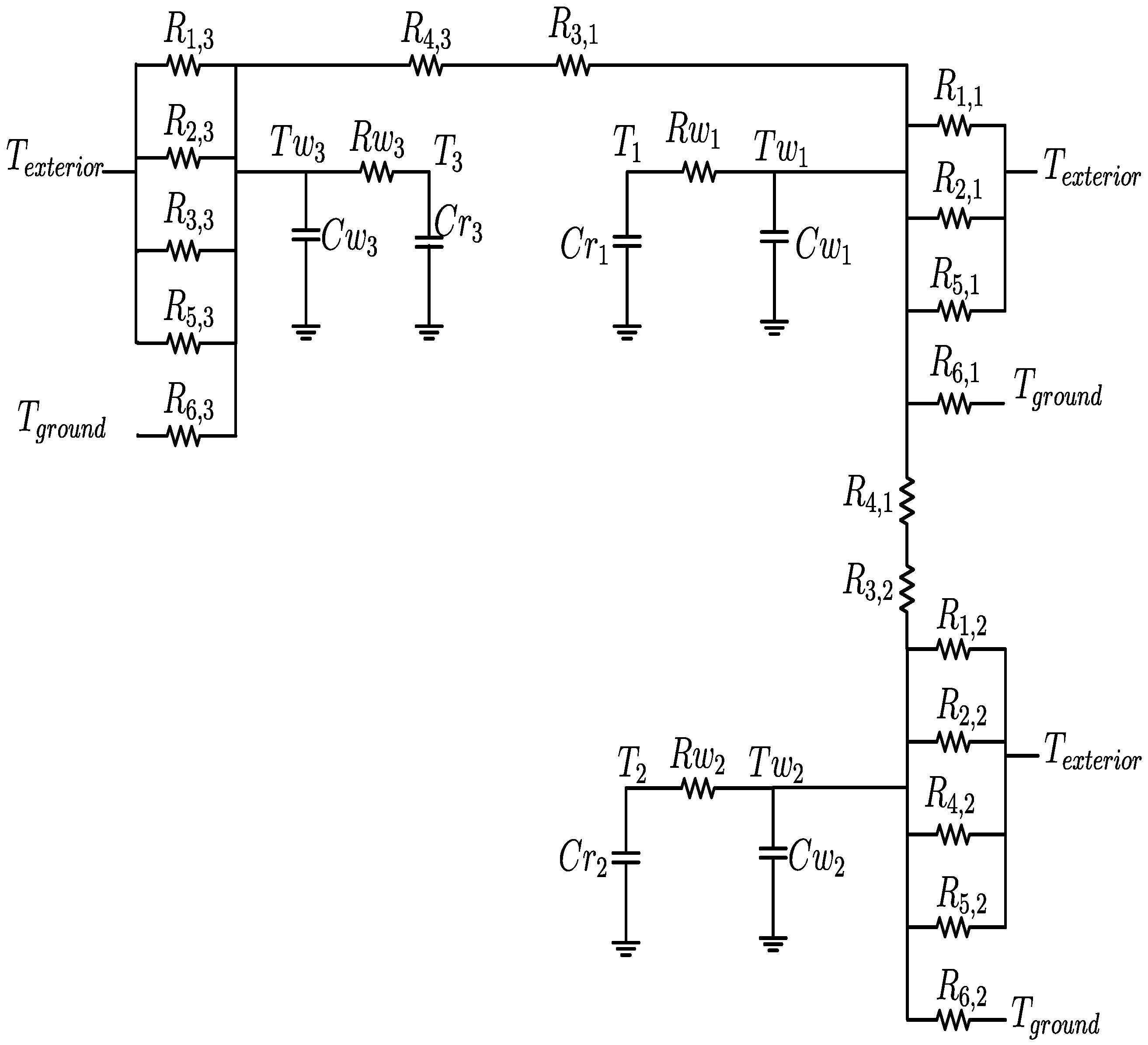
The organization of three thermal zones is presented in Figure 6. In this case, thermal zone 1 is next to two independent zones, zone 2 on the left and zone 3 on the right.
Following the same process described in the two previous cases, the circuit designed for this configuration is presented in Figure 7. Resistors three and four in zone 1 are dedicated to linking the first thermal zone to the adjacent zones. Six differential equations ( N = 6 ) are required to model this circuit, which are derived and presented in the following set of equations:
C w 3 T w 3 ˙ = T 3 R w 3 1 R w 3 + 1 R 1 , 3 + 1 R 2 , 3 + 1 R 3 , 3 + 1 R 4 , 3 + R 3 , 1 + 1 R 5 , 3 + 1 R 6 , 3 T w 3 + T w 1 R 4 , 3 + R 3 , 1 + 1 R 1 , 3 + 1 R 2 , 3 + 1 R 3 , 3 + 1 R 5 , 3 + T g r o u n d R 6 , 3
C r 3 T 3 ˙ = T 3 R w 3 + T w 3 R w 3
C w 2 T w 2 ˙ = T 2 R w 2 1 R w 2 + 1 R 1 , 2 + 1 R 2 , 2 + 1 R 3 , 2 + R 4 , 1 + 1 R 4 , 2 + 1 R 5 , 2 + 1 R 6 , 2 T w 2 + T w 1 R 3 , 2 + R 4 , 1 + 1 R 1 , 2 + 1 R 2 , 2 + 1 R 4 , 2 + 1 R 5 , 2 T e x t e r i o r + T g r o u n d R 6 , 2
C r 2 T 2 ˙ = T 2 R w 2 + T w 2 R w 2
C w 1 T w 1 ˙ = T 1 R w 1 + T w 2 R 4 , 1 + R 3 , 2 + T w 3 R 3 , 1 + R 4 , 3 + 1 R 1 , 1 + 1 R 2 , 1 + 1 R 5 , 1 T e x t e r i o r 1 R w 1 + 1 R 1 , 1 + 1 R 2 , 1 + 1 R 3 , 1 + R 4 , 3 + 1 R 4 , 1 + R 3 , 2 + 1 R 5 , 1 + 1 R 6 , 1 T w 1 + T g r o u n d R 6 , 1
C r 1 T 1 ˙ = T 1 R w 1 + T w 1 R w 1
For this case, T w 3 and T 3 correspond to the temperatures of the third thermal zone. In this model, the central thermal zone is influenced by the adjacent zones. This means that each zone can be affected by a maximum number of 6 thermal zones in the current configuration.

2.4. Case 4: Four Thermal Zones ( m = 4)

The last case study is present in Figure 8; in this configuration, thermal zone 1 is influenced by the three adjacent thermal zones, using surfaces 1, 3 and 4 as contact areas and reducing the ambient temperature over the central zone.
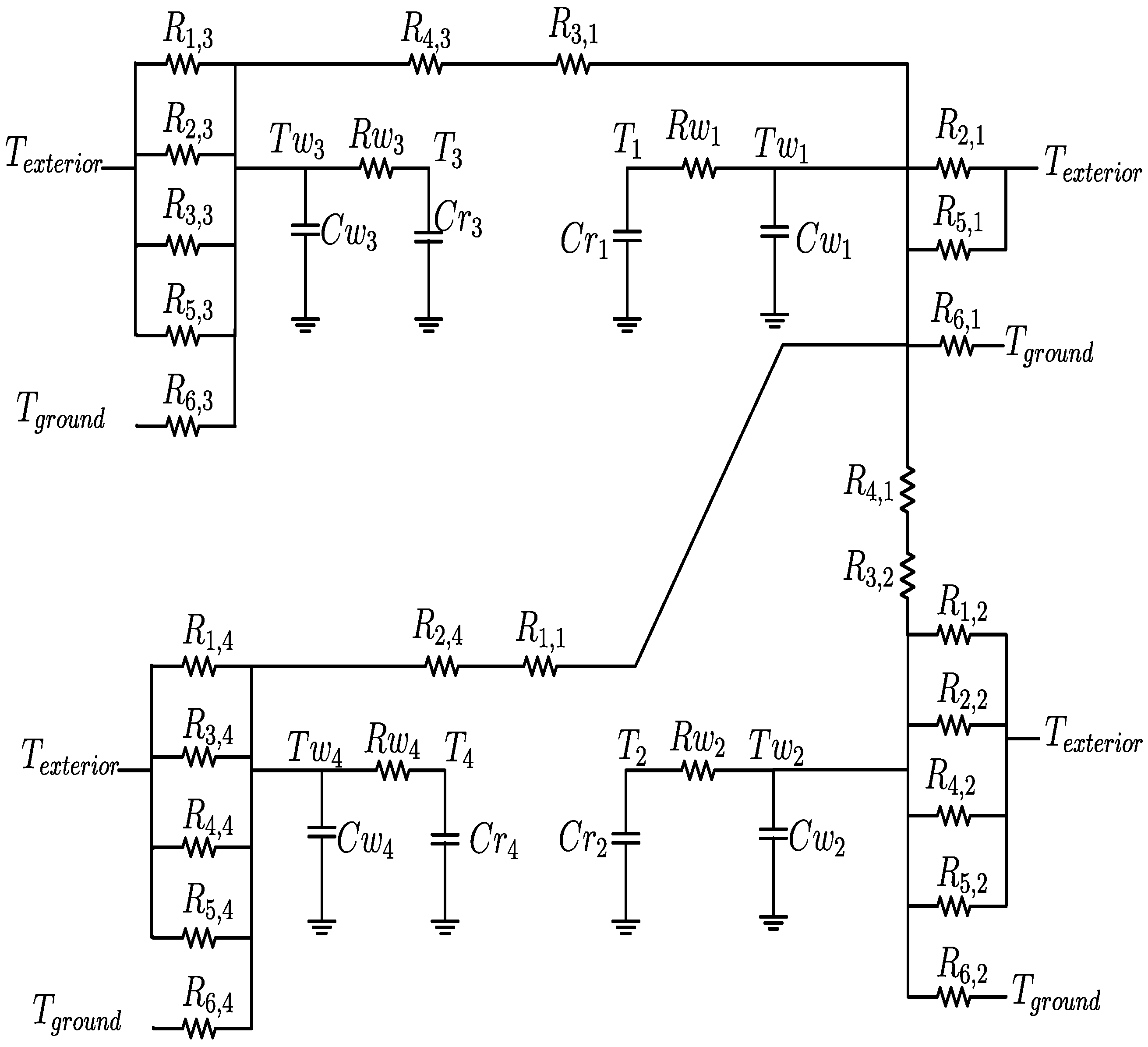
The equivalent circuit for this configuration is shown in Figure 9. In this structure, it is evident that zones 2, 3 and 4 have no effect on each other. The only relationship is an indirect one, using zone 1 as a conductance.
The mathematical model established for this case is present in Equations (19)–(26); it should be noted that only Equation (25) includes the wall temperature of all zones, allowing this zone to be a driver of the indirect relationship between adjacent zones.
C w 4 T w 4 ˙ = T 4 R w 4 1 R w 4 + 1 R 1 , 4 + 1 R 2 , 4 + R 1 , 1 + 1 R 3 , 4 + 1 R 4 , 4 + 1 R 5 , 4 + 1 R 6 , 4 T w 4 + T w 1 R 2 , 4 + R 1 , 1 + 1 R 1 , 4 + 1 R 3 , 4 + 1 R 4 , 4 + 1 R 5 , 4 T e x t e r i o r + T g r o u n d R 6 , 4
C r 4 T 4 ˙ = T 4 R w 4 + T w 4 R w 4
C w 3 T w 3 ˙ = T 3 R w 3 1 R w 3 + 1 R 1 , 3 + 1 R 2 , 3 + 1 R 3 , 3 + 1 R 4 , 3 + R 3 , 1 + 1 R 5 , 3 + 1 R 6 , 3 T w 3 + T w 1 R 4 , 3 + R 3 , 1 + 1 R 1 , 3 + 1 R 2 , 3 + 1 R 3 , 3 + 1 R 5 , 3 T e x t e r i o r + T g r o u n d R 6 , 3
C r 3 T 3 ˙ = T 3 R w 3 + T w 3 R w 3
C w 2 T w 2 ˙ = T 2 R w 2 1 R w 2 + 1 R 1 , 2 + 1 R 2 , 2 + 1 R 3 , 2 + R 4 , 1 + 1 R 4 , 2 + 1 R 5 , 2 + 1 R 6 , 2 T w 2 + T w 1 R 3 , 2 + R 4 , 1 + 1 R 1 , 2 + 1 R 2 , 2 + 1 R 4 , 2 + 1 R 5 , 2 T e x t e r i o r + T g r o u n d R 6 , 2
C r 2 T 2 ˙ = T 2 R w 2 + T w 2 R w 2
C w 1 T w 1 ˙ = T 1 R w 1 + T w 2 R 3 , 2 + R 4 , 1 + T w 3 R 3 , 1 + R 4 , 3 + T w 4 R 1 , 1 + R 2 , 4 + 1 R 2 , 1 + 1 R 5 , 1 T e x t e r i o r 1 R w 1 + 1 R 1 , 1 + R 2 , 4 + 1 R 2 , 1 + 1 R 3 , 1 + R 4 , 3 + 1 R 4 , 1 + R 3 , 2 + 1 R 5 , 1 + 1 R 6 , 1 T w 1 + T g r o u n d R 6 , 2
C r 1 T 1 ˙ = T 1 R w 1 + T w 1 R w 1
The process described in this section is traditionally used to analyze single and multiple thermal zones [26,40]. In all cases, the model must be adjusted to reproduce the experimental measurements, which can be a complex task depending on the size of the model and the number of parameters considered. In this section, different numbers of thermal zones were presented, starting with a single m = 1 zone up to m = 4 , moving from a 2 × 2 to an 8 × 8 system, increasing the tuning complexity and allowing for a more significant percentage error with respect to the experimental data.

3. Algorithm Design

The mathematical models presented in Section 2 and constructed manually require time and effort, but in the case of changes in the position of the thermal zones, steps 2 and 3 must be repeated.
A mathematical modeling algorithm was developed to avoid this problem, using the evidenced pattern. A pair of differential equations was added to the system for each thermal zone in all cases. The structure of these equations is presented in Equations (27) and (28). In this structure, the coefficients α , β and ϕ , which correspond to the impact of adjacent zones, the environment and the ground temperature in each zone, must be calculated.
C w j T w j ˙ = T j R w j + z = 1 m α z T w z + β T e x t e r i o r + ϕ T g r o u n d
C r j T j ˙ = T j R w j + T w j R w j
To capture the spatial organization of the thermal zones, a matrix called a contact matrix was used. This matrix had the dimensions m × 6 ; each row recorded the information of a different zone, thus the first row had information about zone 1, the second row about the second thermal zone, continuing up to the last thermal zone in row m.
The columns in the contact matrix maintained the surface numbering described in Figure 3, using column 1 to indicate whether there was a thermal zone adjacent to the front surface, column 2 to record the existence of a thermal zone on the rear surface and continuing this assignment for all six surfaces; in case there was no adjacent thermal zone, the elements in the column for these directions were replaced by zero.
u = u 1 , 1 u 1 , 2 u 1 , 3 u 1 , 6 u 2 , 1 u 2 , 2 u 2 , 3 u 2 , 6 u m , 1 u m , 2 u m , 3 u m , 6
Equation (29) illustrates the structure of the contact matrix. Using the thermal zone configurations presented in Section 2, the contact matrices were built:
u m = 1 = 0 0 0 0 0 0
u m = 2 = 0 0 0 2 0 0 0 0 1 0 0 0
u m = 3 = 0 0 3 2 0 0 0 0 1 0 0 0 0 0 0 1 0 0
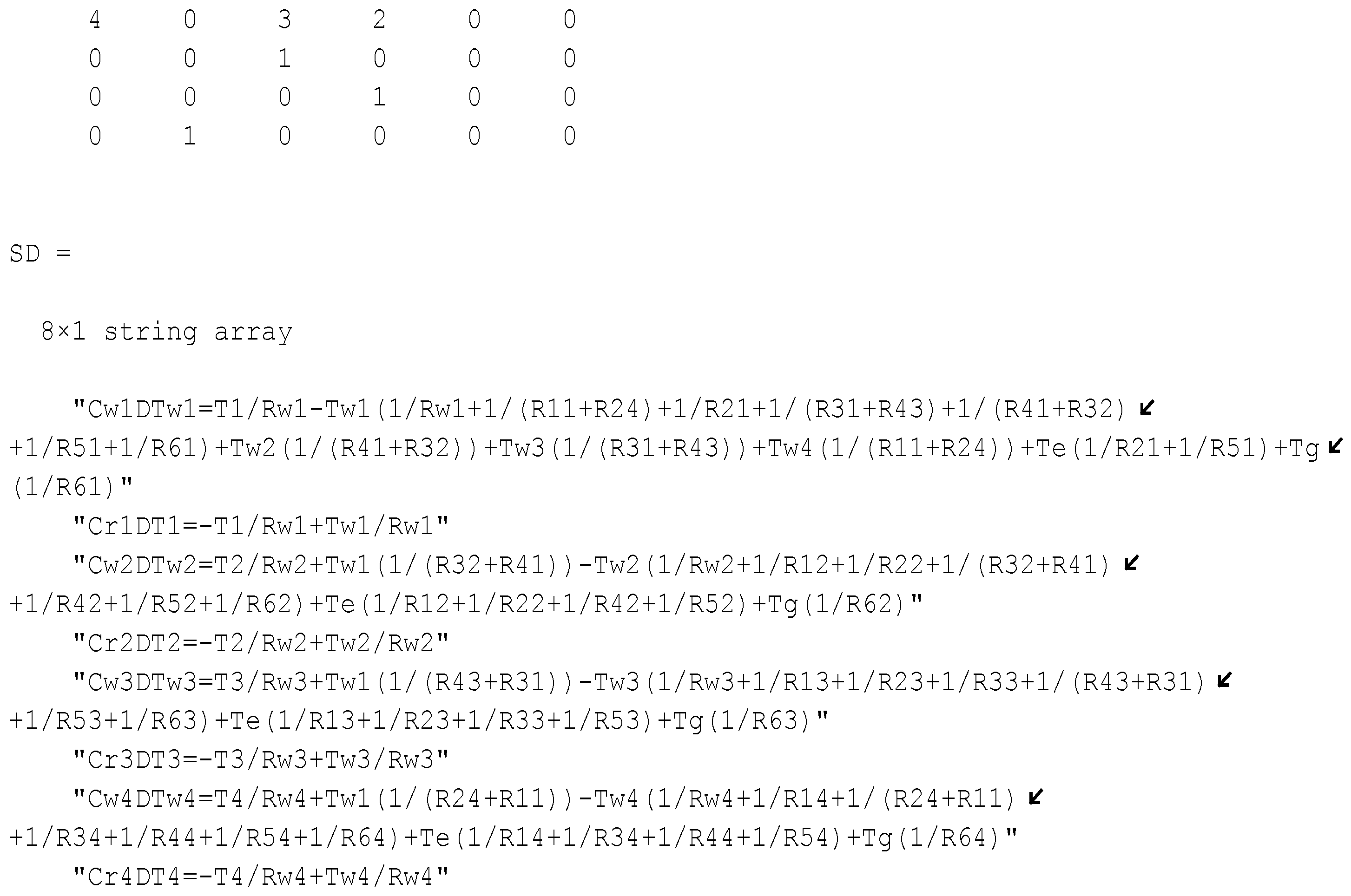
u m = 4 = 4 0 3 2 0 0 0 0 1 0 0 0 0 0 0 1 0 0 0 1 0 0 0 0
We had zone 4 adjacent to wall 1, so element u ( 1 , 1 ) was 4; zone 3 was adjacent to the right surface in zone 1 and for this reason, u ( 1 , 3 ) was 3; and applying the same logic, zone 2 was adjacent to the left surface in zone 1, so u ( 1 , 4 ) = 2 . The zeros represented the surfaces not connected to the thermal zones in the contact matrix. Rows 2, 3 and 4 contained information about zones 2, 3 and 4. In these cases, the only adjacent zone was zone 1; for this reason, most of the spaces were filled with zeros, and the position of zone 1 indicated the position of the first thermal zone with respect to the current zone.
Using the number of thermal zones m, the contact matrix u, the resistances R i , j and the geometrical and physical parameters as inputs, Algorithm 1 was used to determine the differential equations for modeling the multiple-thermal-zone system.
The objective of the algorithm was to generate a pair of equations for each thermal zone, so the β , ϕ and α coefficients had to be determined for each pair of equations. However, they were initially assumed to be zero, and using the information from the contact matrix, they were recalculated.
The coefficient β represented all surfaces in contact with the outside air and contained the sum of the corresponding resistances. The coefficient ϕ was exclusively dedicated to regulate the heat transfer with the ground. Finally, the coefficients α summarized the influence of adjacent thermal zones on the current zone. However, there was a special case, the condition for i = j , where this coefficient summarized the impact of the thermal walls on the interior temperature. In case of walls without connection with other thermal zones, only their own resistance was considered; for this purpose, the δ function was used, using the following behavior:
δ ( x ) = 1 x = 0 0 x 0
The constant k 1 grouped resistors for the walls with no connection to other zones, while the constant k 2 grouped resistors with adjacent zones.
Algorithm 1 Algorithm to design differential equation systems for multiple thermal zones
Energies 16 02247 i001

4. Experimental Development

To evaluate the behavior of the algorithm, a set of experimental tests was executed. Each test was designed to verify the different cases modeled in section two. These models were corroborated by the algorithm presented. The algorithm was programmed in MATLAB software and its results are presented in Appendix A.
The case study selected to evaluate the mathematical models was that of multiple thermal zones made with balsa wood. The physical and geometrical parameters are shown in Table 1.
We used x, y and z as the horizontal length, depth and height of the thermal zone. L d and L w represented the door and wall thickness, respectively. The physical parameters were the density ( ρ ), specific heat ( C e ) and thermal conductivity ( k t ) [43].
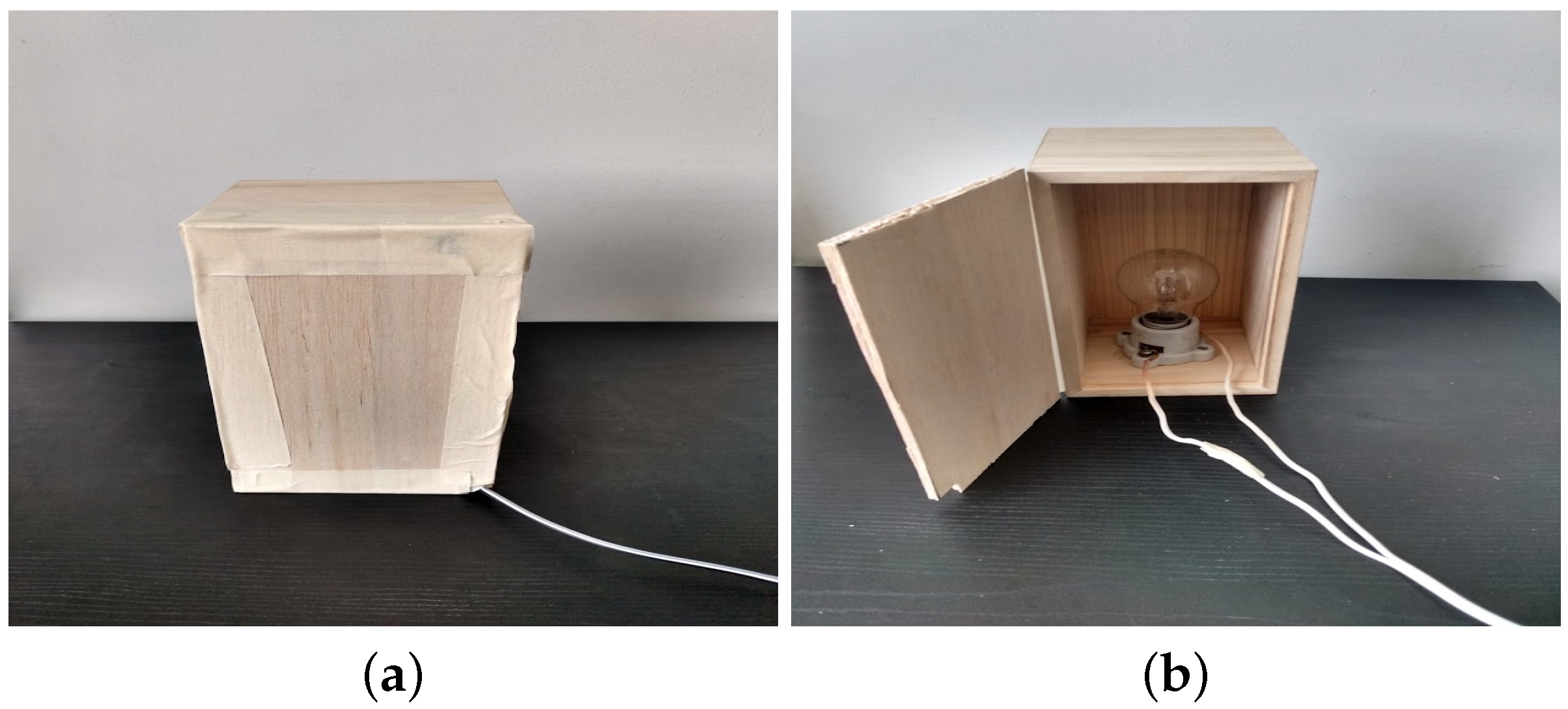
The experiment was run in various stages, increasing the number of thermal zones according to the case studies. In all cases, thermal zone 1 was equipped with an internal heating load. Figure 10 shows a 100 W incandescent bulb as the heat source.
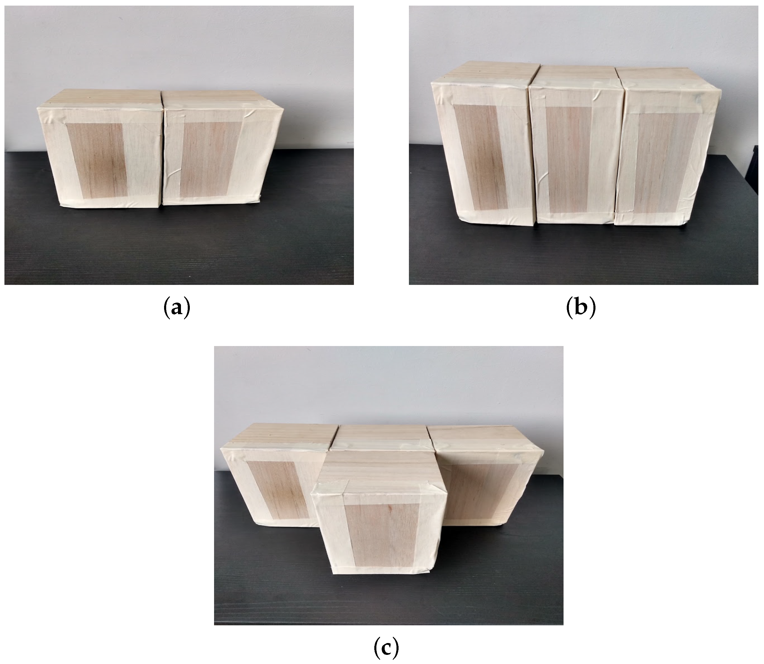
Figure 11 shows the construction of multiple thermal zones according to cases 2, 3 and 4. In addition, each thermal zone had a DHT11 temperature sensor to record the internal temperature, and an additional sensor was dedicated to recording the ambient temperature.
The tests were conducted between 22 and 25 March 2021. Four databases were constructed, one for each case, in which charging processes were carried out with the internal heat source activated for 5 min then turned off and the thermal zones allowed to discharge, releasing the heat to the environment for 30 min.

Tuning Process

In order for the mathematical model to represent the phenomenon under study, a tuning process was carried out. The tuning process had two parts, the first one consisted of calculating fixed values, such as conduction resistances and thermal capacities. These parameters depended on fixed characteristics, such as geometrical and physical characteristics. The second part was dedicated to tuning the variable parameters, i.e., the heat transfer coefficients h e and h i . Each surface could calculate these coefficients, but in this work, it was assumed that all surfaces in a single thermal zone had the same coefficients h e and h i .
The pattern search algorithm was used to adjust the heat transfer coefficients, taking as objective function the error between the experimental data and the simulated results. The fitting process was performed for the loading and unloading phases independently, allowing a different set of coefficients for each phase and thermal zone.
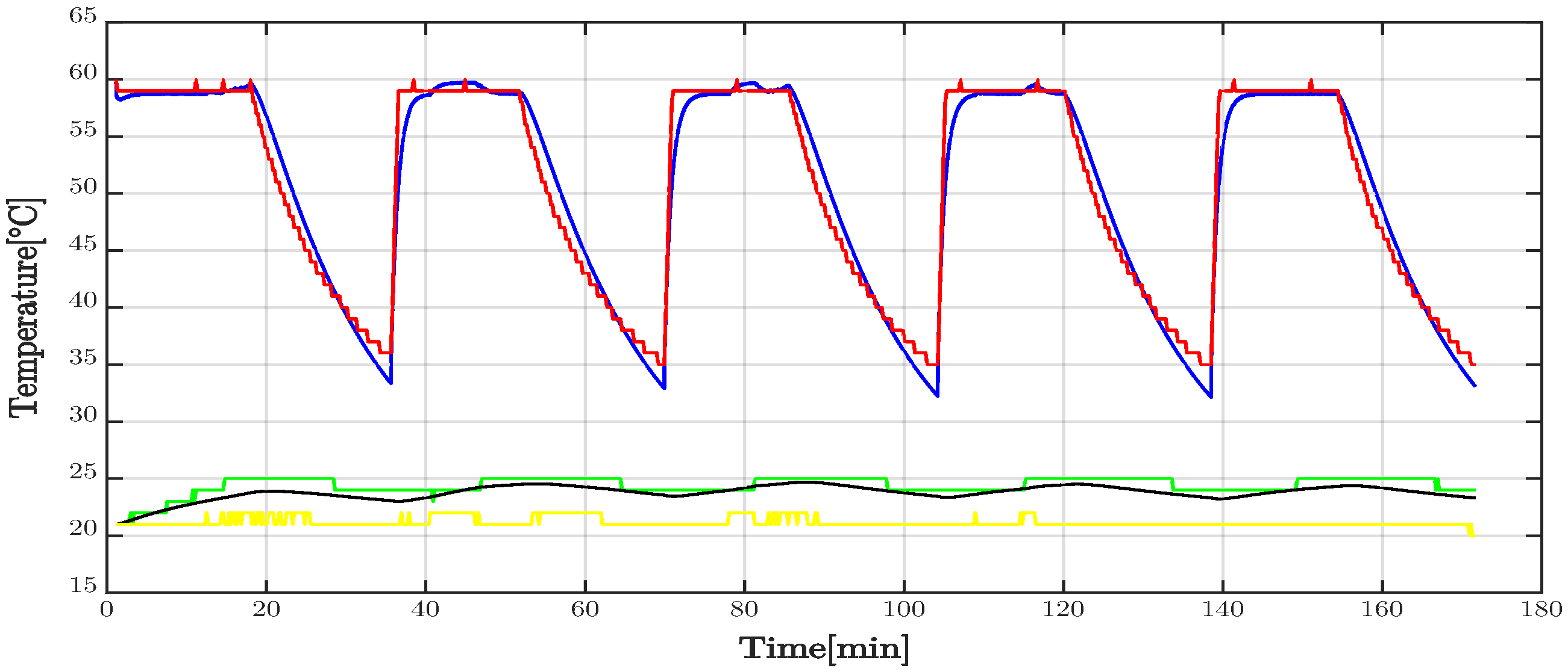
Using the experimental database, the model was fitted for case 1. The results are presented in Figure 12, using a red line to represent the experimental data. The blue line represents the simulated results and finally, the green line is used to represent the ambient temperature. In that case, the error rate between experimental data and simulations was 2.0896 % over 3 h of processing.
Figure 13 shows the internal temperatures for two thermal zones, case 2. The blue and red lines represent the experimental and simulated temperature for zone 1. In addition, the green and black lines denote the experimental and simulated internal temperature in zone 2. In this case, the objective function used for the tuning process was the sum of the experimental and simulated results for each zone, i.e., F o b j e c t i v e = e 1 + e 2 , using e 1 as the percentage error for zone 1 and e 2 the error for zone 2. The errors obtained were 2.94% and 2.97 % for zone 1 and zone 2, respectively.
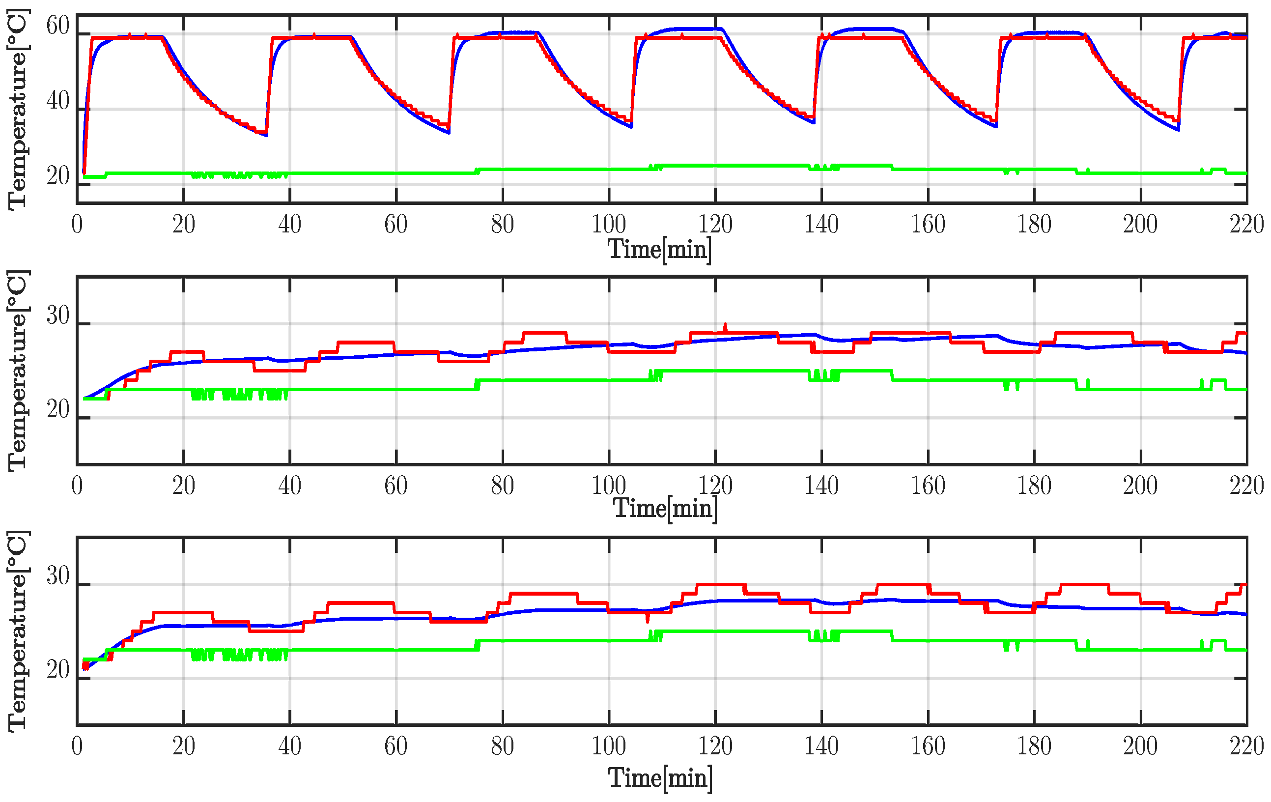
The results of the study on case 3 are presented in Figure 14. In that graph, the first row represents the internal temperature for zone 1, using the blue line for the simulation and the red line for the experiment, and the green line illustrates the environmental temperature. Similarly, the second and third rows represent the simulated and experimental temperatures for zones 2 and 3, respectively. For the case m = 3 , the objective function used was F o b j e c t i v e = i = 1 m e i , considering the error rate simultaneously for the three zones and obtaining e 1 = 3.97 % , e 2 = 3.7 % and e 3 = 4.88 % for each thermal zone.
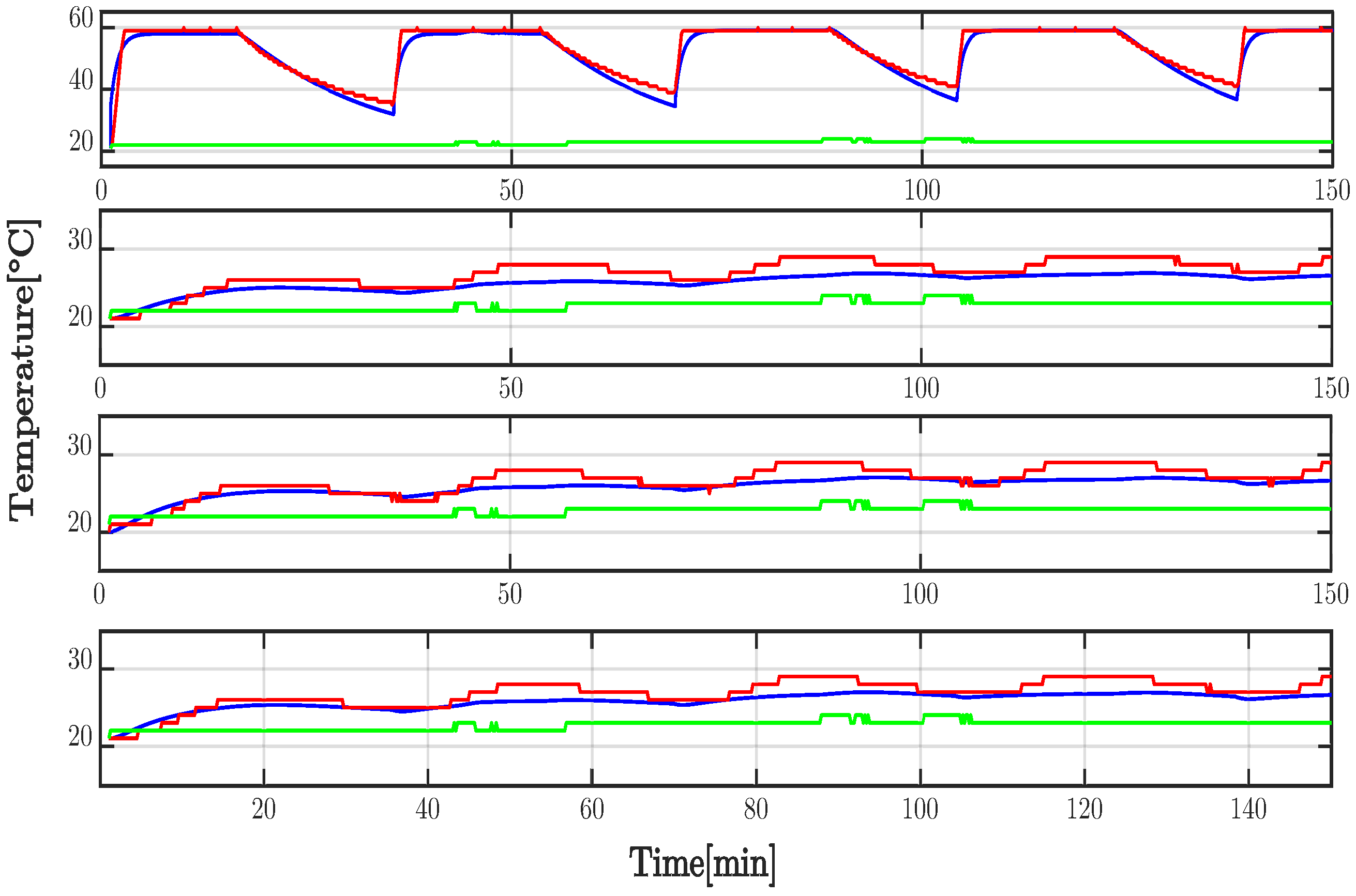
The last case studied ( m = 4 ) is presented in Figure 15. In that figure, the first row shows the temperature for thermal zone 1, the second, third and fourth rows are dedicated to thermal zones 2, 3 and 4, respectively. The blue line corresponds to the simulation and the red line to the experimental results. The green lines represent the ambient temperature. The errors between the experimental and simulated temperature were e 1 = 4.37 % , e 2 = 5.6 % , e 3 = 4.86 % and e 4 = 4.9 % .
The mathematical model was tuned for the charging and discharging process. Table 2 shows the coefficients for the charging phase, explaining the coefficients used in each case. Similarly, Table 3 shows the heat transfer coefficients for the discharge process.
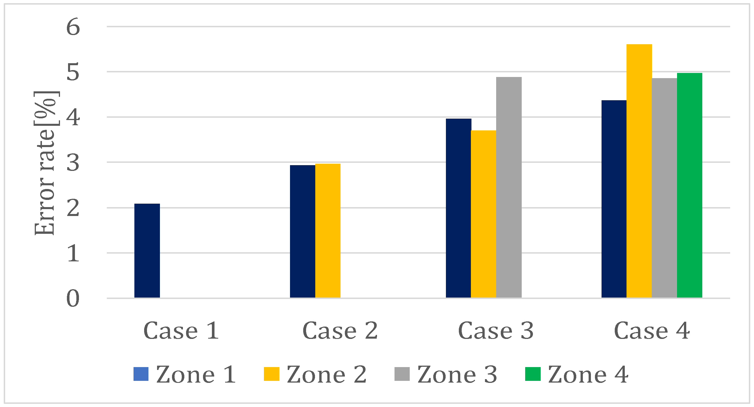
Figure 16 shows the comparison between the different errors calculated for each case. In all cases, the chosen objective function ( F o b j e c t i v e = i = 1 m e i ) allowed us to simultaneously tune the multiple heat transfer coefficients seeking to reduce the error between simulation and experimental results in each case.
Considering all error percentages equally valuable implied that all errors were minimized without emphasizing any one. On the other hand, the error obtained, for example in thermal zone 1, which was reused in all cases, showed a higher error percentage. This problem could be solved by implementing a function for the fitting process.

5. Discussion

In real applications, most offices and houses are composed of multiple thermal zones connected by walls, windows or doors. This situation drives research to formulate and use multiple-thermal-zone models. This paper described an algorithm to generate mathematical models for systems with equal geometry and materials.
The model used to evaluate the mathematical model was an arrangement of wooden boxes in a laboratory space with limited sources of error. However, in real applications, the system can contain multiple heat sources with fixed and variable power, such as windows, doors and occupants. In these cases, heat sources can function as new sources of error that reduce the accuracy of the model and hinder the fitting process. In addition, in residential or larger buildings, the internal air temperature can vary due to internal and external phenomena. For example, the stratification produced by the natural organization of indoor air according to its temperature is especially evident in areas with a high roof. External conditions can produce a high-convection process on a single wall, resulting in a temperature imbalance in the thermal zone. This situation can be corrected by using IR systems or specific ventilation systems that regulate the thermal energy between the different thermal zones.

6. Conclusions

The study of buildings with multiple thermal zones involves the generation of large mathematical models. In this work, an algorithm for the automatic generation of mathematical models was proposed. Initially, a manual process of model generation was presented, considering four cases.
The paper presented the modeling of four systems with multiple thermal zones used as case studies. In each case the organization of the thermal zones, the equivalent electrical circuit and the set of differential equations that represented them were described. The calculation process for all elements of the equivalent electrical circuit was described, including fixed physical parameters such as density, conductivity and specific heat. Additionally, variable physical parameters such as convection coefficients were included, which depended on the conditions under which the experiment was recorded and therefore had to be adjusted for each case. The objective of this process was to demonstrate the complexity of analyzing systems with multiple thermal zones and then compare it with the use of the proposed algorithm.
The proposed algorithm was designed to use the growth pattern in the previously calculated differential equations and allowed us to directly formulate the set of differential equations without drawing the equivalent circuit and circuit analysis. The main input of the algorithm was the contact matrix, an array containing the geometric position of all individual zones according to the nomenclature defined in this article.
A set of experimental tests was used to calibrate the mathematical model generated by the proposed algorithm. These experiments were based on thermal zones with balsa wood for the walls and an internal heat source to ensure energy transfer between the different thermal zones and the environment. The experiments were conducted indoors to reduce the environmental impact. The four systems with multiple thermal zones studied previously were experimentally represented. In each case, the individual zones were equipped with temperature sensors.
The tuning process for the heat transfer coefficient of all thermal zones was carried out using the error temperature, considering the difference between the simulation and experimental data. The best error results was about 2.08 % for a single thermal zone. Meanwhile, the maximal error was 5.6 % obtained in the case of four thermal zones. That error increase can be a problem with a bigger number of zones but can be solved using a better objective function in the tuning process. It is expected to be possible to improve the tuning process in future works and obtain small errors even if large numbers of thermal zones are used.
The internal and external convection coefficient were adjusted in each case. The experiment with a single thermal zone obtained the best error rate between the experimental data and the simulations, obtaining a 2.0896 % error. The second experiment with two thermal zones yielded an average error of 2.95 % . The third experiment showed errors in each thermal zone of 3.97 % , 3.7 % and 4.88 % . Finally, the experiment with four zones showed larger errors in each individual zone, reaching an error of 5.6 % .
With the appropriate fitting process, the mathematical models generated with the proposed algorithm can represent any combination of thermal zones, providing the information is in the format of contact matrices. For the case of systems consisting of parallelepipeds, the proposed algorithm can be a useful tool.

Author Contributions

Conceptualization and methodology, P.F.d.C. and J.T.; experimental development and data collection, R.S. and J.T.; data analysis and simulations F.F.M.; writing—original draft preparation, R.S. and F.F.M.; funding acquisition, P.F.d.C. and R.S.; Writing and editing, M.E.I.M. and J.G.C. The authors consider that all of them contributed equally to this work. All authors have read and agreed to the published version of the manuscript.

Funding

This research received no external funding.

Informed Consent Statement

Not applicable.

Data Availability Statement

Not applicable.

Acknowledgments

Miguel E. Iglesias Martínez’s acknowledges the postdoctoral research scholarship “Ayudas para la recualificación del sistema universitario español 2021–2023. Modalidad: Margarita Salas”, UPV, Ministerio de Universidades, Plan de Recuperación, Transformación y Resiliencia, Spain. Funded by the European Union-Next Generation EU. Pedro Fernández de Córdoba acknowledges the grant PID2021-128676OB-I00 funded by FEDER/MCIN.

Conflicts of Interest

The authors declare no conflict of interest.

Abbreviations

The following abbreviations are used in this manuscript:
HVACHeat, ventilation and air conditioning
LPMLumped-parameter model
RCResistor and capacitor circuit
Nomenclature
ASuperficial area m 2
C e Specific heat kJ kg · K
C r Air thermal capacity kJ K
C w Walls’ thermal capacity kJ K
eError rate%
F o b j e c t i v e Objective function
h i Internal heat convection kJ h · m · K
h e External heat convection kJ h · m · K
k t Thermal conductivity kJ h · m 2 · K
LThicknessm
mThermal zones number
NNumber of equations
RConduction thermal resistance h · K kJ
R i n Internal convection resistance h · K kJ
R e x External convection resistance h · K kJ
R w Inner envelope walls h · K kJ
uContact matrix
TInternal temperature°C
T w Walls’ temperature°C
T e x t e r i o r Environmental temperature°C
T g r o u n d Ground temperature°C
α Heat transfer coefficient between zones kJ h · K
β Heat transfer coefficient with environmental conditions kJ h · K
ϕ Heat transfer coefficient with ground kJ h · K
ρ Density kg m 3

Appendix A

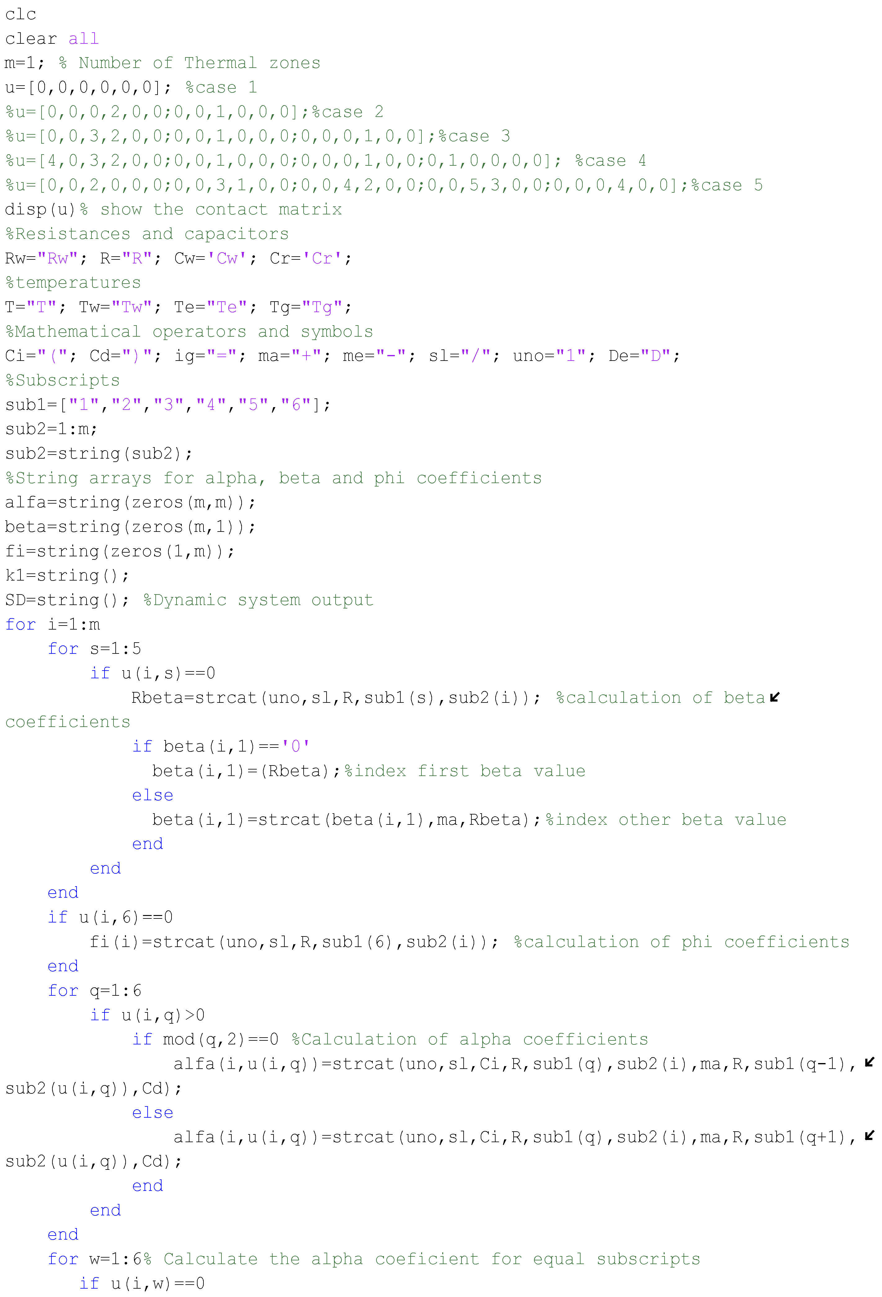
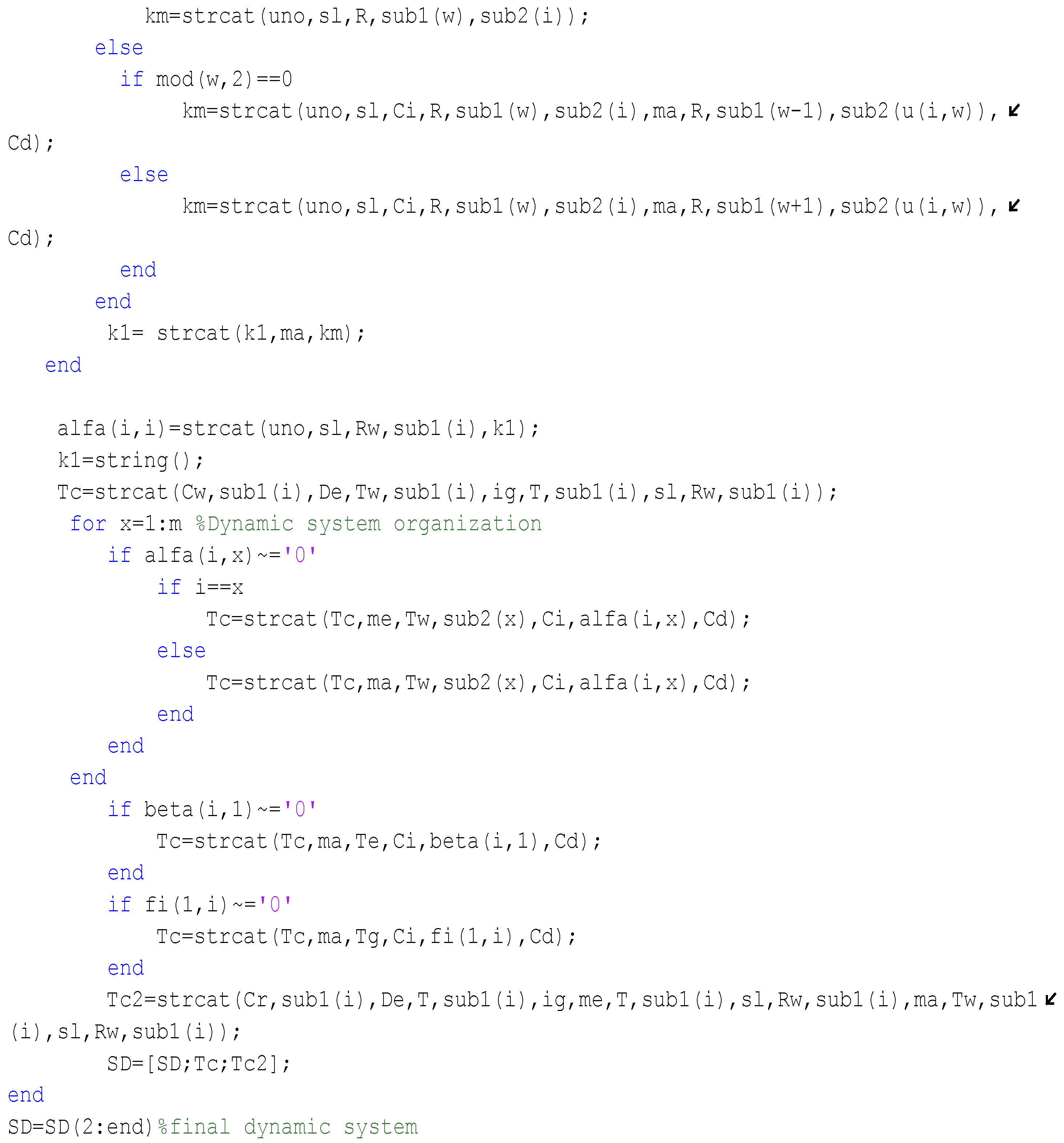
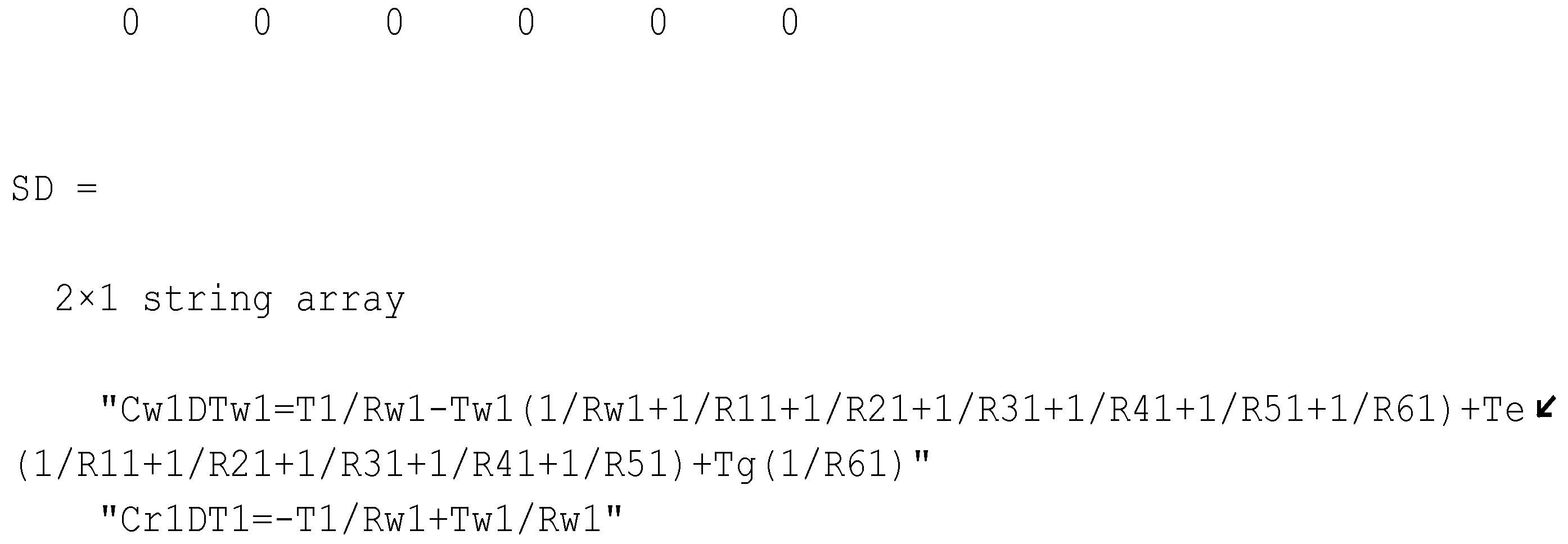
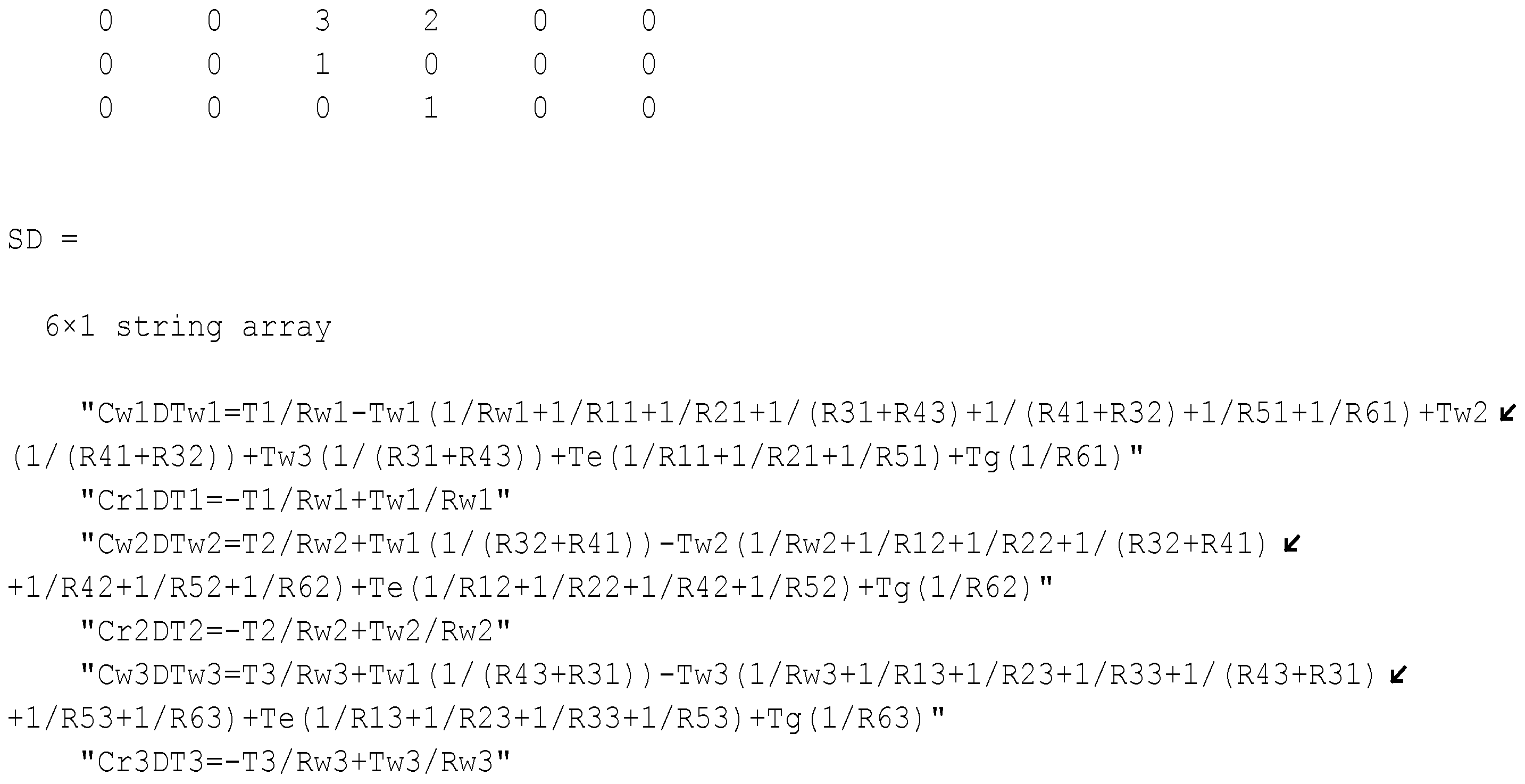
The algorithm to generate the mathematical models was coded in a Matlab file. Figure A1 and Figure A2 show the code used for each specific case with different thermal zones and contact matrices. The algorithm results for each study case are presented in Figure A3, Figure A4, Figure A5 and Figure A6. In all cases, the contact matrix is presented before the mathematical model. These differential equations are string arrays used for building the mathematical model. For the simulation process, the resistances and capacitors must be adjusted to real values.
Figure A1. Code to generate mathematical models (part a).
Energies 16 02247 g0a1
Figure A2. Code to generate mathematical models (part b).
Energies 16 02247 g0a2
Figure A3. Case 1: Mathematical model for a single thermal zone.
Energies 16 02247 g0a3
Figure A4. Case 2: Mathematical model for a double thermal zone.
Energies 16 02247 g0a4
Figure A5. Case 3: Mathematical model for three thermal zones.
Energies 16 02247 g0a5
Figure A6. Case 4: Mathematical model for four thermal zones.
Energies 16 02247 g0a6

References

  1. Czerniawski, T.; Leite, F. Automated digital modeling of existing buildings: A review of visual object recognition methods. Autom. Constr. 2020, 113, 103131. [Google Scholar] [CrossRef]
  2. Deb, C.; Schlueter, A. Review of data-driven energy modelling techniques for building retrofit. Renew. Sustain. Energy Rev. 2021, 144, 110990. [Google Scholar] [CrossRef]
  3. Hou, D.; Hassan, I.G.; Wang, L. Review on building energy model calibration by Bayesian inference. Renew. Sustain. Energy Rev. 2021, 143, 110930. [Google Scholar] [CrossRef]
  4. Lu, D.B.; Warsinger, D.M. Energy savings of retrofitting residential buildings with variable air volume systems across different climates. J. Build. Eng. 2020, 30, 101223. [Google Scholar] [CrossRef]
  5. United Nations. The 2030 Agenda for Sustainable Development; United Nations: New York, NY, USA, 2016. [Google Scholar] [CrossRef]
  6. United Nations. The Paris Agreement; ONU: New York, NY, USA, 2016; pp. 78–79. [Google Scholar]
  7. Li, W.; Wang, S.; Koo, C. A real-time optimal control strategy for multi-zone VAV air-conditioning systems adopting a multi-agent based distributed optimization method. Appl. Energy 2021, 287, 116605. [Google Scholar] [CrossRef]
  8. Biyik, E.; Kahraman, A. A predictive control strategy for optimal management of peak load, thermal comfort, energy storage and renewables in multi-zone buildings. J. Build. Eng. 2019, 25, 100826. [Google Scholar] [CrossRef]
  9. Harputlugil, T.; de Wilde, P. The interaction between humans and buildings for energy efficiency: A critical review. Energy Res. Soc. Sci. 2021, 71, 101828. [Google Scholar] [CrossRef]
  10. Li, Z.; Zhang, J. Study on the distributed model predictive control for multi-zone buildings in personalized heating. Energy Build. 2021, 231, 110627. [Google Scholar] [CrossRef]
  11. Cockroft, J.; Cowie, A.; Samuel, A.; Strachan, P. Potential energy savings achievable by zoned control of individual rooms in UK housing compared to standard central heating controls. Energy Build. 2017, 136, 1–11. [Google Scholar] [CrossRef] [Green Version]
  12. Florez Montes, F. Análisis Dinámico del Confort en Edificios: Estrategias de Control Adaptativo en Modos Deslizantes. Ph.D. Thesis, Universidad Nacional de Colombia and Univertsitat Politècnica de València, Valencia, Spain, 2020. [Google Scholar]
  13. Gunay, H.B.; Shi, Z.; Newsham, G.; Moromisato, R. Detection of zone sensor and actuator faults through inverse greybox modelling. Build. Environ. 2020, 171, 106659. [Google Scholar] [CrossRef]
  14. Alwisy, A.; BuHamdan, S.; Gül, M. Evidence-based ranking of green building design factors according to leading energy modelling tools. Sustain. Cities Soc. 2019, 47, 101491. [Google Scholar] [CrossRef]
  15. Gao, X.W.; Liu, H.Y.; Ruan, B. Discontinuous zone free element method with variable condensation and applications in thermal-stress analysis of functionally graded material structures with cracks. Comput. Struct. 2021, 243, 106411. [Google Scholar] [CrossRef]
  16. Tian, W.; Sevilla, T.A.; Zuo, W.; Sohn, M.D. Coupling fast fluid dynamics and multizone airflow models in Modelica Buildings library to simulate the dynamics of HVAC systems. Build. Environ. 2017, 122, 269–286. [Google Scholar] [CrossRef]
  17. Amin, U.; Hossain, M.J.; Fernandez, E. Optimal price based control of HVAC systems in multizone office buildings for demand response. J. Clean. Prod. 2020, 270, 122059. [Google Scholar] [CrossRef]
  18. Berger, J.; Guernouti, S.; Woloszyn, M.; Chinesta, F. Proper Generalised Decomposition for heat and moisture multizone modelling. Energy Build. 2015, 105, 334–351. [Google Scholar] [CrossRef]
  19. Ng, L.C.; Musser, A.; Persily, A.K.; Emmerich, S.J. Multizone airflow models for calculating infiltration rates in commercial reference buildings. Energy Build. 2013, 58, 11–18. [Google Scholar] [CrossRef]
  20. Garnier, A.; Eynard, J.; Caussanel, M.; Grieu, S. Predictive control of multizone HVAC systems in non-residential buildings. IFAC Proc. Vol. IFAC PapersOnline 2014, 19, 12080–12085. [Google Scholar] [CrossRef] [Green Version]
  21. Żabnieńska-Góra, A.; Khordehgah, N.; Jouhara, H. Annual performance analysis of the PV/T system for the heat demand of a low-energy single-family building. Renew. Energy 2021, 163, 1923–1931. [Google Scholar] [CrossRef]
  22. Gao, Y.; Li, S.; Fu, X.; Dong, W.; Lu, B.; Li, Z. Energy management and demand response with intelligent learning for multi-thermal-zone buildings. Energy 2020, 210, 118411. [Google Scholar] [CrossRef]
  23. Wang, Z.; Liu, J.; Zhang, Y.; Yuan, H.; Zhang, R.; Srinivasan, R.S. Practical issues in implementing machine-learning models for building energy efficiency: Moving beyond obstacles. Renew. Sustain. Energy Rev. 2021, 143, 110929. [Google Scholar] [CrossRef]
  24. Killian, M.; Mayer, B.; Kozek, M. Effective fuzzy black-box modeling for building heating dynamics. Energy Build. 2015, 96, 175–186. [Google Scholar] [CrossRef]
  25. Li, Y.; O’Neill, Z.; Zhang, L.; Chen, J.; Im, P.; DeGraw, J. Grey-box modeling and application for building energy simulations—A critical review. Renew. Sustain. Energy Rev. 2021, 146, 111174. [Google Scholar] [CrossRef]
  26. Yu, X.; Georges, L.; Imsland, L. Data pre-processing and optimization techniques for stochastic and deterministic low-order grey-box models of residential buildings. Energy Build. 2021, 236, 110775. [Google Scholar] [CrossRef]
  27. Abokersh, M.H.; Spiekman, M.; Vijlbrief, O.; van Goch, T.A.; Vallès, M.; Boer, D. A real-time diagnostic tool for evaluating the thermal performance of nearly zero energy buildings. Appl. Energy 2021, 281, 116091. [Google Scholar] [CrossRef]
  28. Brastein, O.M.; Ghaderi, A.; Pfeiffer, C.F.; Skeie, N.O. Analysing uncertainty in parameter estimation and prediction for grey-box building thermal behaviour models. Energy Build. 2020, 224, 110236. [Google Scholar] [CrossRef]
  29. Vivian, J.; Zarrella, A.; Emmi, G.; De Carli, M. An evaluation of the suitability of lumped-capacitance models in calculating energy needs and thermal behaviour of buildings. Energy Build. 2017, 150, 447–465. [Google Scholar] [CrossRef]
  30. Underwood, C.P. An improved lumped parameter method for building thermal modelling. Energy Build. 2014, 79, 191–201. [Google Scholar] [CrossRef] [Green Version]
  31. Parker, S.T.; Williamson, S. Visual assessment of contaminant impacts in multizone buildings. Build. Environ. 2016, 102, 39–53. [Google Scholar] [CrossRef] [Green Version]
  32. Tagade, P.M.; Jeong, B.M.; Choi, H.L. A Gaussian process emulator approach for rapid contaminant characterization with an integrated multizone-CFD model. Build. Environ. 2013, 70, 232–244. [Google Scholar] [CrossRef] [Green Version]
  33. Nguyen, D.H.; Funabashi, T. Decentralized Control Design for User Comfort and Energy Saving in Multi-zone Buildings. Energy Procedia 2019, 156, 172–176. [Google Scholar] [CrossRef]
  34. Subramaniam, M.; Jain, T.; Yame, J.J. Bilinear model-based diagnosis of lock-in-place failures of variable-air-volume HVAC systems of multizone buildings. J. Build. Eng. 2020, 28, 101023. [Google Scholar] [CrossRef]
  35. Ghiaus, C.; Ahmad, N. Thermal circuits assembling and state-space extraction for modelling heat transfer in buildings. Energy 2020, 195, 117019. [Google Scholar] [CrossRef]
  36. Chegari, B.; Tabaa, M.; Simeu, E.; Moutaouakkil, F.; Medromi, H. Multi-objective optimization of building energy performance and indoor thermal comfort by combining artificial neural networks and metaheuristic algorithms. Energy Build. 2021, 239, 110839. [Google Scholar] [CrossRef]
  37. Andrade-Cabrera, C.; Burke, D.; Turner, W.J.; Finn, D.P. Ensemble Calibration of lumped parameter retrofit building models using Particle Swarm Optimization. Energy Build. 2017, 155, 513–532. [Google Scholar] [CrossRef] [Green Version]
  38. Rouchier, S.; Jiménez, M.J.; Castaño, S. Sequential Monte Carlo for on-line parameter estimation of a lumped building energy model. Energy Build. 2019, 187, 86–94. [Google Scholar] [CrossRef]
  39. Dimitriou, V.; Firth, S.K.; Hassan, T.M.; Kane, T. The applicability of Lumped Parameter modelling in houses using in-situ measurements. Energy Build. 2020, 223, 110068. [Google Scholar] [CrossRef]
  40. Lin, Y.; Middelkoop, T.; Barooah, P. Identification of control-oriented thermal models of rooms in multi-room buildings. In Proceedings of the 2012 IEEE 51st Annual Conference on Decision and Control (CDC), Maui, HI, USA, 10–13 December 2013; pp. 1–27. [Google Scholar]
  41. Florez, F.; de Cordoba, P.F.; Taborda, J.; Polo, M.; Castro-Palacio, J.C.; Pérez-Quiles, M.J. Sliding modes control for heat transfer in geodesic domes. Mathematics 2020, 8, 902. [Google Scholar] [CrossRef]
  42. Florez, F.; Córdoba, P.F.D.; Higón, J.L.; Olivar, G.; Taborda, J. Modeling, Simulation, and Temperature Control of a Thermal Zone with Sliding Modes Strategy. Mathematics 2019, 7, 503. [Google Scholar] [CrossRef] [Green Version]
  43. Cengel, Y. Heat and Mass Transfer; John Wiley and Sons: Hoboken, NJ, USA, 2015. [Google Scholar]
Figure 1. Multiple thermal zones located next to each other.
Energies 16 02247 g001
Figure 2. Circuit for a single thermal zone.
Energies 16 02247 g002
Figure 3. Numbering of the walls in a thermal zone.
Energies 16 02247 g003
Figure 4. Two thermal zones.
Energies 16 02247 g004
Figure 5. Circuit for a thermal zone with two places.
Energies 16 02247 g005
Figure 6. Three thermal zones.
Energies 16 02247 g006
Figure 7. Circuit for a thermal zone with three places.
Energies 16 02247 g007
Figure 8. Four thermal zones.
Energies 16 02247 g008
Figure 9. Circuit for a thermal zone with four places.
Energies 16 02247 g009
Figure 10. Thermal zone 1 with internal heating load. (a) Single thermal zone. (b) Single thermal zone with internal load.
Energies 16 02247 g010
Figure 11. Thermal zones for cases 2, 3 and 4 with internal heating load. (a) Case 1. (b) Case 2. (c) Case 3.
Energies 16 02247 g011
Figure 12. Experimental and simulated results for a single thermal zone.
Energies 16 02247 g012
Figure 13. Experimental and simulated results for a double thermal zone.
Energies 16 02247 g013
Figure 14. Experimental and simulated results for three thermal zones.
Energies 16 02247 g014
Figure 15. Experimental and simulated results for four thermal zones.
Energies 16 02247 g015
Figure 16. Error rate for each zone and case studied.
Energies 16 02247 g016
Table 1. Physical and geometrical parameters.
Geometrical Parameters
xyz L d L w
0.111 m0.111 m0.2 m0.005 m0.008 m
Physical Parameters
ρ Cekt
150.7485 kg m 3 3.0512 kJ kg · ° C 0.1882 kJ m · h · ° C
Table 2. Heat transmission coefficients for the charging process.
hi ( kJ h · m · K ) he ( kJ h · m · K )
Zone12341234
Case 186.900012.36000
Case 234.880.00220012.2958.7700
Case 3179.540.0047002.75199.9179.990
Case 437.440.00370.00470.00470.000160.9561.70103.14
Table 3. Heat transmission coefficients for the discharging process.
hi ( kJ h · m · K ) he ( kJ h · m · K )
Zone12341234
Case 10.65760000.0145000
Case 20.00250.001003.3921.4500
Case 30.00270.00180.00027018.650.00080.83870
Case 40.00270.00080.00080.00080.00084.081.894.67
Disclaimer/Publisher’s Note: The statements, opinions and data contained in all publications are solely those of the individual author(s) and contributor(s) and not of MDPI and/or the editor(s). MDPI and/or the editor(s) disclaim responsibility for any injury to people or property resulting from any ideas, methods, instructions or products referred to in the content.