Abstract
Kicks can lead to well control risks during petroleum drilling, and even more serious kicks may lead to serious casualties, which is the biggest threat factor affecting the safety in the process of petroleum drilling. Therefore, how to detect kicks early and efficiently has become a focus practical problem. Traditional machine learning models require a large amount of labeled data, such kicked sample, and it is difficult to label data, which requires a lot of labor and time. To address the above issues, the deep forest is extended to a transfer learning model to improve the generalization ability. In this paper, a transfer learning model is built to detect kicks early. The source domain model adopts the deep forest model. Deep forest is an ensemble learning model with a hierarchical structure similar to deep learning. Each layer contains a variety of random forests. It is an integration of the model in depth and breadth. In the case of a small sample size (20–60 min), kick can be identified 10 min in advance. The deep forest model is established as the source domaining model, and a cascade forest is added at the last layer according to the transfer learning algorithm to form the classification model of this paper. The experimental results show that the kick prediction accuracy of the model is 80.13% by a confusion matrix. In the target domain, the proposed model performs better than other ensemble learning algorithms, and the accuracy is 5% lower than other SOTA transfer learning algorithms.
1. Introduction
Petroleum is an important non-renewable energy. As the blood of industry, petroleum is deeply involved in every aspect of the economy and society. It not only affects peoples’ daily lives, but also is an indispensable strategic resource for national survival and development. There are two main identification methods for kick prediction in actual production. One is to identify the kick situation according to the change in physical quantity, and the other is to predict the kick, leakage, and other risk conditions according to artificial intelligence technology combined with comprehensive logging technology. With the increasing depth of drilling, the geological environment is becoming more and more complex. In the process of drilling, well kick is one of the biggest threats to the safe drilling operation. If not managed properly, a kick can turn into a blowout. It can lead to the abandonment of borehole, causing great economic loss and threatening the lives of drilling workers. The most effective way to control kick is early detection so that the well can be adjusted accordingly to minimize losses. As a result, predicting the occurrence of the kick in advance based on real-time drilling data will provide valuable operational time to prevent and control the kick. This can effectively avoid well control hazards and reduce safety risks.
With the rise of artificial intelligence, machine learning has been applied to various fields, and there are many researches on kick prediction. In 2001, Hargreaves et al. [1] used Bayesian probability framework to determine kick whether or not according to the noise of drilling data, which improved the sensitivity of the system and reduced the false alarm rate. With the discovery of artificial intelligence technology, scholars put forward artificial neural network. In 2012, Moazzeni et al. [2] used artificial neural networks to predict well loss. In 2016, Chiranth Hegde [3] proposed a data-driven model, which can be used as an effective proxy for complex concept modeling in engineering to optimize some controllable input parameters in the model to improve operational efficiency. In 2018, Christine I. Noshi [4] summarized data analysis case studies, workflows, and lessons learned to enable field personnel, engineers, and management to quickly interpret trends, detect failure patterns in operations, diagnose problems, and implement remedial actions to monitor and safeguard operations. In 2019, Xiaodong Wu [5] used BP neural network combined with bee colony algorithm (ABC) to build a deep drilling kick identification model. In 2020, Li Yufei et al. [6] proposed an intelligent kick identification method based on support vector machine (SVM) and a kick comprehensive discrimination method based on improved Dempster–Shafer (D–S) evidence theory, which greatly improved the accuracy of kick compared with the previous single-means SVM method. In the same year, Sergey Borozdin et al. [7] proposed a drilling simulation model. The training efficiency of this model is higher. The latest models were trained to solve regression problems of indicator functions, to track changes in certain parameters through model settings, and to identify anomalies in the drilling process in real time. In 2021, Fattahi et al. [8] used artificial neural network (ANN) and other methods to calculate the drilling rate index, with a high accuracy. In the same year, Sivakumar Mahalingam et al. [9] used the coordinated search algorithm named harmony search algorithm (HSA) to study various features. Mingming He et al. [10] proposed a CNN framework with prediction errors within the acceptable range of physics.
Three questions have been left unanswered by previous research. The first problem is that the use of such methods requires a large amount of data to train the model from scratch, and the acquisition of this data requires a large amount of labor and effort. The second problem is that the data obtained is not balanced, and it still needs to be processed manually. The third problem is that the variation from well to well is very large, and previous studies have not been able to transfer good models to another well with a small amount of data. The model proposed in this paper is designed to solve these problems.
2. Related Work
2.1. Transfer Learning
Transfer learning is not a new concept specific to deep learning. It is a stark difference between the traditional approach of building and training machine models and the methodology of using transfer learning principles. Traditional methods are isolated, purely based on specific tasks, and dataset trains isolated model. No knowledge is retained that can be migrated from one model to another. In transfer learning, we can use previously trained models to gain knowledge (features, weights, etc.), train new models, and even deal with problems with less data for new tasks. Transfer learning should allow us to take what we have learned from previous learning tasks and apply it to new related tasks. If we have significantly more data on task T1, we can take what we have learned and generalize that knowledge (features, weights) to task T2. New environments exist in the real world, and the appearance of new environments in the data usually affects the performance of the model. In order to make full use of the labeled data and ensure the model accuracy on the new data, transfer learning emerged. Transfer learning has been applied in various fields of research, such as natural language processing (NLP), computer vision (CV), and so on. Transfer learning has become a major research direction. In recent years, there are many time series prediction methods based on transfer learning. For example, Hassan Ismail Fawaz et al. [11] proposed the flow forecast framework in 2018, and Yuntao Du [12] proposed the ADARNN model in 2021, which solved the problem of time series covariance drift and so on.
According to the description of Weiss et al. [13], Figure 1 shows the process of transfer learning. The yellow rectangle on the left of Figure 1 represents the training data of field A, and the red rounded rectangle on the right of Figure 1 represents the training data of target domain. These two types of rectangles represent data in two similar domains with similar features. The data of source domain and target domain are similar, but there are some differences. This is the basic condition for transfer. Model A is the model trained with the training data of field A. The knowledge obtained from model A is extracted, such as the feature of the data in Figure 1 (rectangle, green), and used for model B to train the training data in field B. Model B uses the knowledge obtained from model A training (rectangle) to train model B faster.
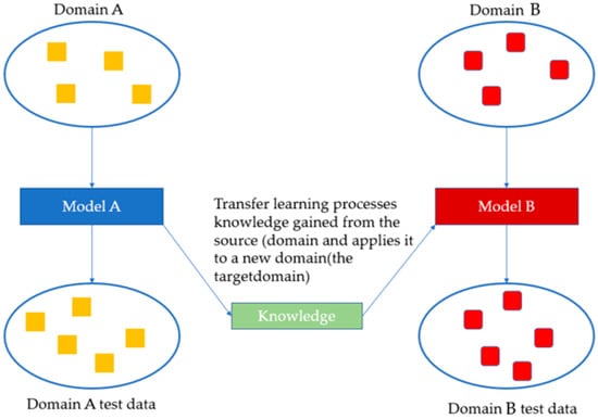
Figure 1.
Structure of Transfer learning.
2.2. Deep Forest
Deep forest is an ensemble model proposed by Zhou in 2018 [14]. As ensemble learning, deep forest can effectively improve the accuracy of prediction. The idea of ensemble learning is to ensemble several individual classifiers when classifying new instances. The final classification is determined by some combination of the classification results of multiple classifiers to achieve better performance than a single classifier. If a single classifier is compared to a decision maker, ensemble learning is equivalent to multiple decision makers making a decision together. So, ensemble learning can improve the accuracy of prediction.
Deep forest is a deep learning-like hierarchical structure (right of Figure 2), where the output of each layer is connected with the raw data to become the input of the next layer. In each layer, there are several cascading random forests, which are made up of decision trees. For diversity, each cascading forest includes two fully random forests and two random forests. Completely random forest is a random selection of features in the complete feature space to split. The main difference between the two kinds of forests is the candidate feature space. In ordinary random forest, the split nodes are selected by Gini coefficient in a random feature subspace.
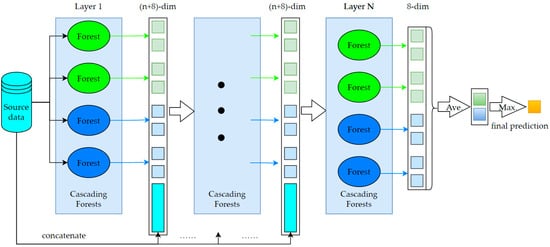
Figure 2.
Structure of Deep Forest.
In this structure, input features are used to train two completely random tree forests and two random forests. The sample label is the actual label of the sample. Each forest training is independently supervised learning. Inside each layer the forest is independent of each other. Each forest outputs two types of probability distributions, equivalent to two new features. These new features are combined with the original input features to form a new input for the next layer. After training a forest at a layer, use the four forests at that layer on the validation set to see if the performance improves. If the improvement is not significant, no new layer is generated. In other words, the iteration stops until the effect does not improve.
Decision tree is the basic element of random forest, and it is a kind of intuitive model. We can think of a decision tree as a series of yes/no questions about the data that ultimately result in a prediction category. It is an interpretable model because it is very similar to how humans think.
A random forest is a model made up of many decision trees. Instead of simply averaging the predictions of all trees, this model uses two key concepts from which the random comes, random sampling of training data points when building a tree and considering random subsets of features when splitting nodes. Due to the existence of randomness, the attributes and characteristics of the data are crossed, so that there is a certain connection between different trees.
Deep forest is shown as Figure 2. The blue rectangle in the figure is the original data, which forms a structure similar to the residual connection with the output of each layer as the input of the next layer. The output of each forest in each layer is a probability distribution, and the output of the last layer will take the maximum probability of the average distribution of the output of all forests as the final output.
3. Dataset
This study adopts the field drilling history data of two wells in one oilfield. Table 1 shows the details of the data.

Table 1.
Descriptive statistics of data.
The data of well No. 1 is used as the source domain selection data, with a total of 25,726 samples, and the kick sample number is 12,207. The data of well No. 2 is used as the target domain data, with a total of 20,292 samples, and the kick sample number is 7046. As the target domain data, it is more consistent with the actual situation with few kick samples. Each sample have 56 features, including pressure, flow, and mechanical parameters. The detailed features of the data are in Table A1 in the Appendix A. They are input into the model as features of multivariate time series.
The model constructed in this paper uses 10 min of drilling data to predict whether kick will occur in the next 10 min, and 50 pieces of data are stored in the drilling site in 1 min. Therefore, the time series of 500 samples are used to predict whether kick will occur in the next 500 samples. So, the predicted result can reflect whether the kick occurs in ten minutes. Figure 3 shows the process of the training set construction. The time window size is ten minutes. As shown in the Figure, the label corresponding to the current time window is whether kick occurs in the next time window. So, the predicted result can reflect whether the kick occurs in 10 min.
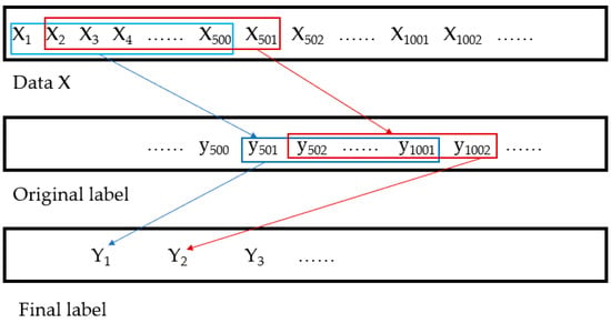
Figure 3.
The process of the training set construction.
4. Methodology
4.1. Source Model Construction
The early detection of kick is essentially a prediction task for time series. Ordinary ensemble learning methods such as Random Forest, XGBoost, and LightGBM have good effects. However, compared with deep learning models such as RNN, the accuracy of ensemble learning methods still needs to be improved. Therefore, combining the advantages of the two kinds of models and the effect of each model on the source domain, the deep forest method is adopted. Deep neural networks rely on the depth of layers to represent the processing of original features. According to the deep neural network, the deep forest is designed as the structure shown in Figure 2, in which each layer of the forest receives the characteristic information, the upper layer processes the information and outputs its processing results to the next layer. Each layer is a collection of decision tree forests. Here, the cascade forest at each level includes different types of forest to ensure diversity, which is essential to the overall construction. For simplicity, suppose we use two completely random tree forests and two random forests. The number of trees per forest is a hyperparameter. Given an instance, each forest will produce an estimate of the class distribution, compute the percentage of training examples of different classes on the leaf nodes where the relevant instances fall, and then average them across all the same trees. The estimated class distribution forms a class vector, which is then connected to input the original feature vector into the next level of the cascade. To reduce the risk of overfitting, the class vectors generated by each forest are cross-checked by K-fold. Specifically, each instance will be used as the training data of k−1 for cross-validation to obtain k−1 class vectors, and then average them to obtain the final result class vector as the enhanced feature of the next cascade. After expanding to a new level, the performance of the entire cascade can be estimated and verified, and if there is no significant performance, the training process will be terminated. Therefore, the number of cascade levels is automatically determined. Deep forest adaptively determines model complexity through termination training. This character allows it to be adapted to different sizes of training data, it is not limited to large-scale.
Each piece of data is fed into the model, and then each forest at each layer outputs a distribution. The distribution is the probability of the label ‘normal’. A forest is a collection of decision trees. A decision tree is like asking a set of yes or no questions to continuously improve the accuracy of a prediction. Each forest distribution as a new feature is then concatenated with the original data. The concatenated data serves as input to the next layer.
4.2. Transfer Learning Framework
Transfer learning has fine-tuned steps, such as freezing some layers, and then modifying some layers or adding new layers. We try to transfer by retraining the last layer of the deep forest or adding new layers according to transfer learning.
To achieve transfer, we choose to fix the weight parameters of the first three layers, and modify the output of the source domain model. We make it the same as the output of each layer, that is, the output distribution of multiple forests. The data of the target domain needs to be distributed through the model output of the source domain. Residuals are then connected to the original model of the target domain. After the new layer is added, the output distribution conforming to the target domain is obtained and the maximum value of the average distribution is taken as the output. Deep forest based on transfer learning is shown as Figure 4.
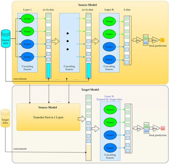
Figure 4.
Deep forest based on transfer learning.
5. Experimental Results
5.1. Experiment Settings
The datasets for the experiment are UCI air quality [15], UCI-Amazon access samples [16], Ecg MIT-BIH database [17], and well data which is mentioned in Section 3. The UCI air quality dataset contains 9358 instances of hourly averaged responses from an array of 5 metal oxide chemical sensors embedded in an air quality chemical multisensor device. UCI-Amazon access sample is a sparse dataset, less than 10% of the attributes are used for each sample. MIT-BIH Noise Stress Test Database involves twelve half-hour ECG recordings and three half-hour recordings of noise typical in ambulatory ECG recordings. The ECG recordings are created by adding calibrated amounts of noise to clean ECG recordings from the MIT-BIH Arrhythmia Database.
The UCI datasets are divided into source and target domains in a ratio of 4:1, and the Ecg data is divided into source and target domains based on individual data. The well data is the data of two wells, one of which is the target domain. Each dataset is divided into 4:1 and 20% as the test set and 80% as the training set. The experimental evaluation metric is the accuracy calculated by confusion matrix. Statistical results are the average of the five times experiments.
5.2. Source Domain Model Selection
First of all, it is necessary to build an excellent source domain model. We conducted experiments with the deep forest model and other models commonly used in time series prediction on common datasets and well data. The experimental results are shown in Table 2.

Table 2.
Source domain results of different models.
It can be seen that the effect of deep forest on the source domain is better than other machine learning methods, and the accuracy of the model is within the expected range.
5.3. Transfer Learning Model
This part of the experiment mainly compares the effect of the proposed model with other commonly used transfer learning models on different time series datasets.
AdaRNN is proposed by Yuntao Du in 2021. It is a new paradigm for time series prediction. In addition, Dann is proposed by Yaroslav Ganin in 2014 which is a depth domain adaptive model. Flow forecast is proposed by Hassan, Ismail Fawaz in 2018. It is a framework model of time series prediction of transfer learning. The above three models have good effect on time series prediction.
The datasets used in the test are multidimensional time series, including UCI-Airquality monitoring data, UCI-Amazon Access Samples, ECG-MIT-BIH, and petroleum data.
Experiments are conducted to test the accuracy and cost of each model in different scenarios. The transfer learning deep forest is conducted by adding a new layer of linked forest after the last layer of the original deep forest.
To verify the necessity of transfer learning, the models in Table 2 are directly to predict on target domain dataset. In other words, we use source domain data for training and target domain data for testing. Table 3 shows the results of these different models.

Table 3.
Target domain results of different models.
As can be seen from Table 3, although the deep forest model is the best among them, the performance of all models is also greatly reduced compared to Table 2. Therefore, transfer learning is needed to improve model performance. Table 4 shows the training accuracy and training cost of each transfer learning model.

Table 4.
Results of accuracy comparison with other transfer learning models.
For the comparison, the Adarnn and Dann can obtain better accuracies on different datasets. The transfer forest achieves the second-best result on all the datasets with the least time cost. Regarding to the datasets, the petroleum dataset owns the most complex features. The results show that the transfer forest has great potential for processing complex data.
Take the 5th sample in Table 1 as an example for analysis. Figure 5 shows the variation of drilling features such as the standpipe pressure, inlet flow, pump stroke and outlet flow over time. Figure 6 is the predicted result for the sample. The ‘orange’ line is the probability of the label ‘normal’. In this experiment, ‘1’ is normal and ‘0’ is kick. The closer the distribution is to ‘1’, the greater the probability that it is normal. Conversely, the closer the distribution is to ‘0’, the more likely it is to kick. The orange line refers to the distribution of the output, compared to the real black line, which can detect the kick in advance. Both false positives and the proposed model can be identified in advance. The blue curve is the outlet flow, and the obvious jitter in the figure is the cause of false positives.
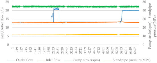
Figure 5.
The drilling features trends of sample 5.
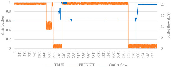
Figure 6.
The kick prediction result of sample 5.
5.4. Ablation Experiment
The two important parameters of a deep forest are the depth and the number of trees because the number of layers in the deep forest is automatically generated, and the generation is terminated by the early stop function. So, we fixed the structure of the deep forest first, and analyzed each tree.
It can be seen in Table 5 that when the number of subtrees is 40, the effect is best, and increasing the number of subtrees will not improve the accuracy of the model. In addition, the number of forests per layer in the deep forest also affects the results. We have conducted the experiments with different numbers of forests in one layer, and the results are show as Table 6.

Table 5.
Model accuracies with different subtrees.

Table 6.
Deep forest performance of different layers and number of random forests.
As can be seen that, when the number of forests is eight, no matter how many layers, the effect is better than others. In order to see the performance changes more intuitively, Figure 7 shows the relationship between the number of layers and accuracy when the number of forests is eight.
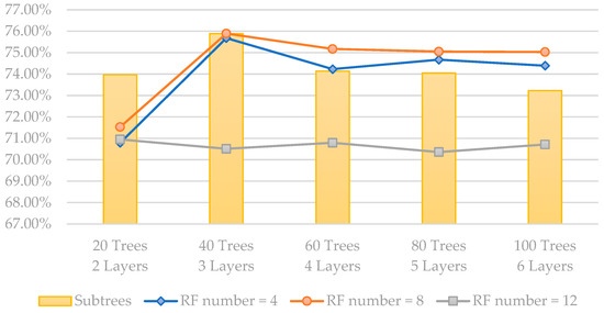
Figure 7.
The relationship between parameters and accuracy.
We can see that the best results are achieved when the number of layers is three and the number of forests in each layer is eight. Then, with above model parameters, we can obtain a good model of source domain.
In order to obtain a better model in target domain, we change the number of the added layers to test the impact on the effect of the transfer. Table 7 and Figure 8 show that adding one layer achieves the best performance on all the metrics. Increasing the amount of layers will not improve the transfer effect.

Table 7.
The newly added layer effects on model accuracy.
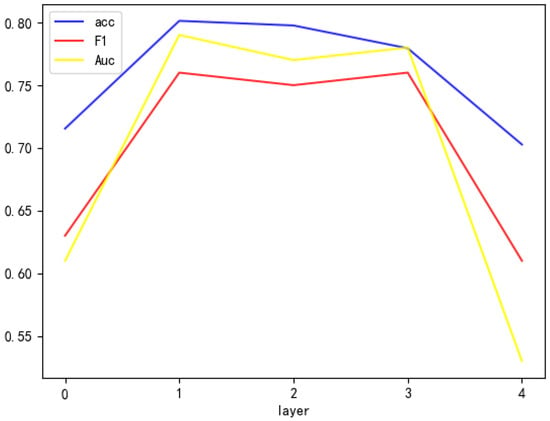
Figure 8.
The newly added layer effects on model accuracy.
5.5. Sample Effects on the Experimen
Training data size is another key factor impacting the transfer effect. Therefore, we have conducted several experiments to verify the effects as Table 8. As we can see from the results, the more training data, the better performance obtains. In the process of actual drilling, when the model is applied to a new well, it is likely that there will be only positive samples. Based on this, splicing the new samples with the old samples is tried. The splicing is positive samples of the target domain combining negative samples of the source domain. However, in actual situations, the negative samples of the new data may be relatively small, so we try to increase the number of positive samples of the new data in order to observe its impact on the results.

Table 8.
Influence of sample shape in target domain on model accuracy.
The results of the spliced samples are much better on average than the unspliced samples. Because the spliced sample includes various information of the target domain sample.
The composition of the normal and kick samples will have a certain impact on the experimental results, in which the larger the proportion of the target domain samples to the spliced samples, the better the effect will be. In addition, the larger the number of samples, the better the experimental results will be. There is no overfitting problem, because every layer of the deep forest will be cross-verified to prevent the overfitting problem.
6. Conclusions
Traditional machine learning requires a large amount of data. A large amount of labeled data require a large amount of labor, high time consumption, and high cost. Moreover, a large amount of labeled data are often difficult to obtain in the production time. In order to solve this problem, this paper proposes the transfer forest. The features and recognition tasks of different wells are the same, but the difference is the feature distribution of data between different wells. Transfer forest can effectively solve the problem of model differences between two wells caused by different scenes. The results show that the transfer forest can predict the drilling kick 10 min in advance, and the accuracy is 80.13%. The model effectively achieves the expected purpose, enhances the generalization ability of the model, ensures the drilling safety, and effectively reduces the probability of well control danger. The transfer forest is a general method which can be used to detect mud lost, well collapse, sticking, and other drilling conditions.
Author Contributions
Conceptualization, W.L.; Data curation, X.Z.; Funding acquisition, X.H.; Investigation, J.F.; Methodology, J.F., W.L., X.Z. and X.H.; Resources, J.F.; Software, X.Z.; Supervision, X.H.; Validation, J.F.; Writing—original draft, J.F., X.Z. and X.H.; Writing—review and editing, W.L. and X.H. All authors have read and agreed to the published version of the manuscript.
Funding
The authors are grateful for the support of the National Key Research and Development Program of China No.2019YFA0708304, the National Natural Science Foundation of China No.61972174 and No.62172187, the Science and Technology Planning Project of Jilin Province No.20220201145GX and No.20220601112FG, the Science and Technology Planning Project of Guangdong Province No.2020A0505100018, Guangdong Universities’ Innovation Team Project No.2021KCXTD015 and Guangdong Key Disciplines Project No.2021ZDJS138, Projects of CNPC No.2021DQ0503 and No. 2020B-4019.
Data Availability Statement
Not applicable.
Conflicts of Interest
The authors declare no conflict of interest.
Appendix A

Table A1.
Feature of data.
Table A1.
Feature of data.
| No. | Feature | No. | Feature | No. | Feature | No. | Feature |
|---|---|---|---|---|---|---|---|
| 1 | Measure depth (m) | 15 | Pump-stroke1 (spm) | 29 | CH4 (%) | 43 | Fixed point pressure (MPa) |
| 2 | True vertical depth (m) | 16 | Pump-stroke2 (spm) | 30 | C2H6 (%) | 44 | Wellhead regulating pressure (MPa) |
| 3 | Bit depth (m) | 17 | Pump-stroke3 (spm) | 31 | PWD true vertical depth (m) | 45 | Fixed point pressure loss (MPa) |
| 4 | Bit vertical depth (m) | 18 | total pit volume (m³) | 32 | PWD Annulus pressure (MPa) | 46 | Fluctuating pressure (MPa) |
| 5 | Average rate of penetration (m/min) | 19 | bottoms up (min) | 33 | PWD Dev (deg) | 47 | Pressure loss correction factor (MPa/km) |
| 6 | Average weight on bit (KN) | 20 | Mud loss (m³) | 34 | PWD direction (deg) | 48 | Drilling speed (m/s) |
| 7 | Hook weight (KN) | 21 | Inlet flow log (L/s) | 35 | Up depth (m) | 49 | Drilling acceleration (m/s²) |
| 8 | Rotary RPM (rpm) | 22 | Outlet flow (L/s) | 36 | MPD_ST | 50 | Fixed-point ECD (g/cc) |
| 9 | Torque (KN.m) | 23 | Inlet flow log (g/cc) | 37 | Loop back pressure (MPa) | 51 | Bit ECD (g/cc) |
| 10 | Kelly down (m) | 24 | Outlet flow log (g/cc) | 38 | Inlet flow (L/s) | 52 | Drill string pressure drop (MPa) |
| 11 | Hook position (m) | 25 | Inlet temperature (°C) | 39 | Fixed depth (m) | 53 | Bit pressure drop (MPa) |
| 12 | Hook speed (m/s) | 26 | Outlet temperature (°C) | 40 | Fixed vertical depth (m) | 54 | Annulus pressure loss (MPa) |
| 13 | Standpipe pressure log (MPa) | 27 | Total hydrocarbon (%) | 41 | Back pressure pump (L/s) | 55 | Target back pressure (MPa) |
| 14 | Casing pressure (MPa) | 28 | H2S (ppm) | 42 | Standpipe pressure (MPa) | 56 | Hydrostatic pressure (MPa) |
References
- Hargreaves, D.; Jardine, S.; Jeffryes, B. Early Kick Detection for Deepwater Drilling: New Probabilistic Methods Applied in the Field. In Proceedings of the SPE Annual Technical Conference and Exhibition, New Orleans, LA, USA, 30 September 2001; p. SPE-71369-MS. [Google Scholar]
- Moazzeni, A.; Nabaei, M.; Jegarluei, S. Decision Making for Reduction of Nonproductive Time through an Integrated Lost Circulation Prediction. Pet. Sci. Technol. 2012, 30, 2097–2107. [Google Scholar] [CrossRef]
- Hegde, C.; Gray, K.E. Use of Machine Learning and Data Analytics to Increase Drilling Efficiency for Nearby Wells. J. Nat. Gas Sci. Eng. 2017, 40, 327–335. [Google Scholar] [CrossRef]
- Noshi, C.; Schubert, J. The Role of Machine Learning in Drilling Operations; A Review. In Proceedings of the SPE/AAPG Eastern Regional Meeting, Pittsburgh, PA, USA, 7–11 October 2018. [Google Scholar]
- Wu, X.D. Early Overflow Monitoring and Identification Technology for Deepwater Drilling. Master’s Thesis, China University of Petroleum, Beijing, China, 2019. [Google Scholar]
- Li, Y.F.; Zhang, B.; Sun, W.F. Research on Intelligent Early Kick Identification Method Based on SVM and D-S Evidence Theory. Drill. Prod. Technol. 2020, 43, 27–30. [Google Scholar]
- Borozdin, S.; Dmitrievsky, A.; Eremin, N.; Arkhipov, A.; Sboev, A.; Chashchina-Semenova, O.; Fitzner, L.; Safarova, E. Drilling Problems Forecast System Based on Neural Network. In Proceedings of the SPE Annual Caspian Technical Conference, Virtual, 21–22 October 2020. [Google Scholar]
- Fattahi, H.; Bazdar, H. Applying Improved Artificial Neural Network Models to Evaluate Drilling Rate Index. Tunn. Undergr. Space Technol. 2017, 70, 114–124. [Google Scholar] [CrossRef]
- Mahalingam, S.; Balaji, K.; Natarajan, Y. Multi-Objective Soft Computing Approaches to Evaluate the Performance of Abrasive Water Jet Drilling Parameters on Die Steel. Arab. J. Sci. Eng. 2021, 46, 7893–7907. [Google Scholar] [CrossRef]
- He, M.; Zhang, Z.; Li, N. Deep Convolutional Neural Network-Based Method for Strength Parameter Prediction of Jointed Rock Mass Using Drilling Logging Data. Int. J. Geomech. 2021, 21, 04021111. [Google Scholar] [CrossRef]
- Ismail Fawaz, H.; Forestier, G.; Weber, J.; Idoumghar, L.; Muller, P.-A. Transfer Learning for Time Series Classification. In Proceedings of the 2018 IEEE International Conference on Big Data (Big Data), Seattle, WA, USA, 10–13 December 2018; pp. 1367–1376. [Google Scholar]
- Du, Y.; Wang, J.; Feng, W.; Pan, S.; Qin, T.; Xu, R.; Wang, C. AdaRNN: Adaptive Learning and Forecasting of Time Series. In Proceedings of the 30th ACM International Conference on Information & Knowledge Management; Association for Computing Machinery, New York, NY, USA, 30 October 2021; pp. 402–411. [Google Scholar]
- Pan, S.J.; Yang, Q. A Survey on Transfer Learning. IEEE Trans. Knowl. Data Eng. 2010, 22, 1345–1359. [Google Scholar] [CrossRef]
- Zhou, Z.-H.; Feng, J. Deep Forest. Natl. Sci. Rev. 2019, 6, 74–86. [Google Scholar] [CrossRef] [PubMed]
- De Vito, S.; Massera, E.; Piga, M.; Martinotto, L.; Di Francia, G. On Field Calibration of an Electronic Nose for Benzene Estimation in an Urban Pollution Monitoring Scenario. Sens. Actuators B Chem. 2008, 129, 750–757. [Google Scholar] [CrossRef]
- Dua, D.; Graff, C. UCI Machine Learning Repository; School of Information and Computer Science, University of California: Irvine, CA, USA, 2017; Available online: https://archive.ics.uci.edu/ml/datasets/Amazon+Access+Samples (accessed on 1 September 2022).
- Goldberger, A.L.; Amaral, L.A.N.; Glass, L.; Hausdorff, J.M.; Ivanov, P.C.; Mark, R.G.; Mietus, J.E.; Moody, G.B.; Peng, C.-K.; Stanley, H.E. PhysioBank, PhysioToolkit, and PhysioNet. Circulation 2000, 101, e215–e220. [Google Scholar] [CrossRef] [PubMed]
Disclaimer/Publisher’s Note: The statements, opinions and data contained in all publications are solely those of the individual author(s) and contributor(s) and not of MDPI and/or the editor(s). MDPI and/or the editor(s) disclaim responsibility for any injury to people or property resulting from any ideas, methods, instructions or products referred to in the content. |
© 2023 by the authors. Licensee MDPI, Basel, Switzerland. This article is an open access article distributed under the terms and conditions of the Creative Commons Attribution (CC BY) license (https://creativecommons.org/licenses/by/4.0/).