Load Frequency Control and Automatic Voltage Regulation in Four-Area Interconnected Power Systems Using a Gradient-Based Optimizer

Abstract

Existing interconnected power systems (IPSs) are being overloaded by the expansion of the industrial and residential sectors together with the incorporation of renewable energy sources, which cause serious fluctuations in frequency, voltage, and tie-line power. The automatic voltage regulation (AVR) and load frequency control (LFC) loops provide high quality power to all consumers with nominal frequency, voltage, and tie-line power deviation, ensuring the stability and security of IPS in these conditions. In this paper, a proportional integral derivative (PID) controller is investigated for the effective control of a four-area IPS. Each IPS area has five generating units including gas, thermal reheat, hydro, and two renewable energy sources, namely wind and solar photovoltaic plants. The PID controller was tuned by a meta-heuristic optimization algorithm known as a gradient-based optimizer (GBO). The integral of time multiplied by squared value of error (ITSE) was utilized as an error criterion for the evaluation of the fitness function. The voltage, frequency, and tie-line power responses of GBO-PID were evaluated and compared with integral–proportional derivative (GBO-I-PD), tilt integral derivative (GBO-TID), and integral–proportional (GBO-I-P) controllers with 5% step load perturbation (SLP) provided in each of the four areas. Comprehensive comparisons between GBO-PID and other control methodologies revealed that the proposed GBO-PID controller provides superior voltage, frequency, and tie-line power responses in each area. The reliability and efficacy of GBO-PID methodology were further validated with variations in the turbine time constant and speed regulation over a range of  ± 25%. It is evident from the outcomes of the sensitivity analysis that the proposed GBO-PID control methodology is very reliable and can successfully stabilize the deviations in terminal voltage, load frequency, and tie-line power with a shorter settling time in a four-area IPS.

1. Introduction

Modern power networks are undergoing a rapid transformation due to the proliferation of diverse renewable energy sources and smart grid technologies. The most crucial control objective in power systems is to manage the output power in such a way that the frequency deviation, terminal voltage deviation, and interchange power between areas is zero. The automatic voltage regulator (AVR) and load frequency control (LFC) strategies are responsible for the generation and supply of consistent and reliable power in an interconnected power system (IPS), while keeping the frequency and voltage within acceptable limits. The load in a power system is always dynamic and it continually changes. The imbalance between generation and load demand causes an extremely undesirable change in the system’s frequency and voltage. By adjusting the active power demand through the speed governor action of the LFC control loop, the frequency deviation is controlled. The deviation in terminal voltage is regulated by adjusting the reactive power demand through the generator excitation of the AVR loop. It is a very challenging problem to design an intelligent and robust control methodology that can successfully minimize the variations in terminal voltage and system frequency by regulating the tie-line power flow. Designing a controller with an accurate tuning scheme is very important for the optimal control of an IPS. In this study, an effort is made for the effective control of LFC and AVR systems in a four-area IPS utilizing a nature-inspired computation-based control strategy [1,2].

The AVR and LFC controllers have gained significant importance for the smooth operation of modern and complex power networks in recent past. For instance, Tayyab Ali et al. proposed LPBO-, AOA-, and MPSO-based PI-PD controllers for a multi-area IPS. When the responses of existing NLTA-PID and proposed PI-PD-based control schemes were tested, it was discovered that the proposed methodology performed significantly better than traditional controllers [1]. Tayyab Ali et al. also studied the behavior of multiarea, multisource IPS with different nonlinearities including GRC, BD, and GDB using a DO-based PI-PD controller. The obtained results clearly revealed that the suggested control schemes effectively minimized the voltage, frequency, and tie-line power deviations [2]. Chandrakala and Balamurugun used a PID controller tuned with simulated annealing (SA) and a traditional Ziegler–Nichols (ZN) technique to stabilize the two-area IPS. They were effective in controlling the load frequency and the terminal voltage [3]. To improve time response, Gupta and Srivastava investigated the hybrid NN-FTF controller for voltage and frequency stabilization in a single-area power system [4]. Devashish Sharma et al. recommended ZN-based FLC and PID controllers for a single-area, single-source IPS. It was discovered that the system’s dynamic response is enhanced in terms of peak overshoots, oscillation damping, and settling time [5]. Rumi and Lalit explored PIDF/PIDuF controllers based on LSA to analyze the behavior of a two-area, four-source nonlinear IPS that includes GRC, GDB, SMES, and IPFC. When compared to other traditional methods, the use of a fractional-order controller with a filter produced superior results [6]. The FOPID controller for two-area nonlinear IPS was investigated by Deepak and Ajit. The optimal parameters of the FOPID controller were discovered using MFO [7]. A. K. Sahani et al. proposed a PID controller based on FA for a two-area, four-source IPS with hydro and non-reheat thermal generation units. While accomplishing ideal transients, they successfully stabilized the power system [8]. The IPSO-based CPSS controller for single-area nonlinear IPS was proposed by Javed and Zahra. Their power system model combines hydro, thermal reheat, and gas production units [9]. Naga Sai Kalyan and Sambasiva examined a DE-AEFA-based PID control scheme for a two-area IPS in the presence of nonlinearities such as GRC. In order to achieve significant improvements, the power system additionally included the IPFC, RFBs, and HVDC link [10,11]. Abhineet and Parida suggested SCA-based PI and PIDF controllers for AVR and LFC loops, respectively, with non-reheat and thermal reheat generation units. The combined application of a unified power flow controller (UPFC) and redox flow battery (RFB) ensured further improvements in the system’s response [12]. Nabil Nahas et al. developed a PID controller for a two-area linear IPS. PID was effectively optimized by using NLTA [13]. Naga Sai Kalyan presented a GWO-based PIDD controller for a two-area nonlinear IPS. The design also took into account UPFC and SMES [14]. Pachunoori Anusha et al. investigated a PID controller tuned with FA in a two-area, four-source IPS with nonlinearities, including GDB, TD, and GRC [15]. Stephen Oladipo et al. used a PIDA controller tuned with hFPAPFA for a single-area, single-source IPS. FPA and PFA in conjunction have been investigated to improve system performance and provide a global best solution [16]. For a three-area, two-sources nonlinear IPS, an HHO-tuned TIDF controller was also suggested by researchers [17]. Sheikh Safiullah et al. studied the second-order error-driven control-law -based ADRC controller for a three-area IPS. This system uses EVs, solar, geothermal, and wind as generation sources [18]. An HHO-based 2DOF I-TDF controller with dish-stirling, wind, solar, and reheat thermal generation units was also advised by Satish Kumar Ramoji et al. for three-area, two-source nonlinear IPS. When the response of the suggested controller was compared with TID, TIDF, and I-TDF, it was shown to be superior to the others [19]. For a three-area IPS in the presence of GDB and GRC nonlinearities, Biswanath Dekaraja suggested a CFPD-TID controller based on AFA. The effect of high voltage DC links and RFBs on system dynamics was also highlighted in that study [20]. For a two-area, four-source nonlinear IPS in the presence of CTD, GDB, and GRC, Biswanath Dekaraja et al. presented a CFOTDN-FOPDN controller designed with AFA [21]. In [22], Biswanath Dekaraja employed an AFA-based CPDN-FOPIDN controller in a three-area IPS that had GDB and GRC nonlinearities. The performance of the system was further enhanced by the addition of an HVDC link and multiple energy storage components. For a two-area, ten-source IPS with three bioenergy and two solar energy sources, Hady H. Fayek and Eugen Rusu investigated a PIDA controller using DPO [23]. Naga Sai Kalyan et al. investigated a HAEFA-based fuzzy PID for a two-area, three-source IPS that included energy storage devices such as RFBs, SMES, and UCs. The simulation findings show that ESDs may be successfully integrated into the LFC-AVR system and RFBs are superior at attenuating frequency and voltage oscillations [24].

Table 1. Summary of previous combined AVR-LFC studies.

Reference of Paper	Area of Research	Tuning Method	Suggested Controller	Generation Sources	Year	Generation Sources in All Areas	Covered Area	Additional Incorporation for Improvements	Nonlinearities
[1]	LFC and AVR	AOA, LPBO, MPSO	PI-PD	-	2022	2, 3	2, 3	-	-
[2]	LFC and AVR	DO	PI-PD	Reheat thermal, Hydro, and Gas	2022	6	2, 3	-	GDB, BD, GRC
[3]	LFC and AVR	SA, ZN	PID	Hydro and Non-reheat thermal	2016	4	2	-	GDB
[4]	LFC and AVR	NN-FTF	Hybrid NN and FTF	-	2016	1	1	-	-
[5]	LFC and AVR	ZN, FLC	PID, Fuzzy	-	2018	1	1	-	-
[6]	LFC and AVR	LSA	PIDF, PIDuF	Reheat thermal, Wind, and Diesel	2018	4	2	IPFC, SMES	GDB, GRC
[7]	LFC and AVR	MFO	FOPID	Hydro and Non-reheat thermal	2019	4	2	-	GDB, BD
[8]	LFC and AVR	FA	PID	Hydro and Non-reheat thermal	2019	4	2	-	-
[9]	LFC and AVR	IPSO	CPSS	Gas, Reheat thermal, and Hydro	2020	1	1	-	GDB, GRC
[10]	LFC and AVR	DE-AEFA	PID	Wind , Hydro, Thermal, Gas, Solar, and Diesel	2020	6	2	HVDC link	GRC
[11]	LFC and AVR	DE-AEFA	PID	Gas, Diesel, Hydro, Solar photovoltaic, Reheat thermal, and Wind	2020	6	2	IPFC, RFBs	GRC
[12]	LFC and AVR	SCA	PIDF, PI	Reheat thermal and Non-reheat thermal	2020	2	2	UPFC, RFBs	-
[13]	LFC and AVR	NLTA	PID	-	2021	2	2	-	-
[14]	LFC and AVR	GWO	PIDD	Reheat thermal, Hydro, and Nuclear	2021	6	2	SMES, UPFC	GRC, GDB
[15]	LFC and AVR	FA	PID	Reheat thermal and Hydro	2021	4	2	-	TD, GRC, GDB
[16]	LFC and AVR	hFPAPFA	PIDA	Thermal	2021	1	1	-	-
[17]	LFC and AVR	HHO	TIDF	Reheat thermal and Combined cycle gas turbine (CCGT)	2021	6	3	-	GDB, GRC, BD
[18]	LFC and AVR	2nd order error-driven control law	ADRC	Solar, Geothermal, Wind, and EVs	2022	6	3	-	-
[19]	LFC and AVR	HHO	2DOF I-TDF	Reheat thermal, Wind, Solar thermal, and Dish-stirling,	2022	6	3	-	GDB, GRC
[20]	LFC and AVR	AFA	CFPD-TID	Hydro, Thermal, and Geothermal	2022	6	3	RFBs, HVDC link	GRC, DB
[21]	LFC and AVR	AFA	CFOTDN-FOPDN	Hydro, Dish-stirling, Solar thermal, and Reheat thermal	2022	4	2	-	GDB, CTD, GRC
[22]	LFC and AVR	AFA	CPDN-FOPIDN	Reheat thermal, Hydro, Gas, and Geothermal	2022	6	3	FESS, CES, RFBs, SMES HVDC link	GRC, GDB
[23]	LFC and AVR	DPO	PIDA	Three Bioenergy technologies and two Solar energy sources	2022	10	2	-	-
[24]	LFC and AVR	HAEFA	Fuzzy PID	Reheat thermal, Hydro, and Gas	2022	6	2	UCs, SMES, RFBs	-
Proposed Method	LFC and AVR	GBO	PID	Thermal, Gas, Hydro, Wind, and Solar	2022	20	4	-	-

lists the literature on combined LFC-AVR in a summarized form. Compared to combined LFC-AVR studies, individual LFC research is much more extensive. For example, nature-inspired computation algorithms such as the fitness dependent optimizer (FDO), improved fitness dependent optimizer (I-FDO), and hybrid sine cosine algorithm with FDO (hSC-FDO) have been explored for the optimal control of the LFC loop up to a two-area IPS using different controllers such as FO-ITD, FO-ITDN, FO-I-PD, I-PD, etc. [25,26,27,28,29,30]. Moreover, different control strategies have been presented for individual control of the AVR loop [31,32,33,34,35]. Researchers have presented many nature-inspired computation algorithms in the recent past to solve different engineering problems [36,37,38,39,40,41,42,43]. Numerous research investigations have been carried out for the individual and combined control of AVR and LFC systems in a multiarea environment. There exists a huge literature on the individual study of LFC or AVR loops, but very few studies were found on the combined control of LFC and AVR systems due to the highly complicated structure of IPS. To the best of our knowledge, a four-area IPS with five generation units in each area is not yet explored. This served as the motivation for looking into a four-area IPS having five generation units in each area, including two renewable energy sources, i.e., solar and wind photovoltaic systems. The gradient-based optimizer (GBO) has been explored to acquire optimal gain parameters for the proposed PID and for other controllers such as I-PD, TID, and I-P. This research brings a new look to the existing literature for the control of IPSs, as most of the presented control methodologies consider up to two- or three-area IPSs. The proposed control method for a four-area IPS will definitely extend the research on these complex IPSs. This work’s key contributions are:

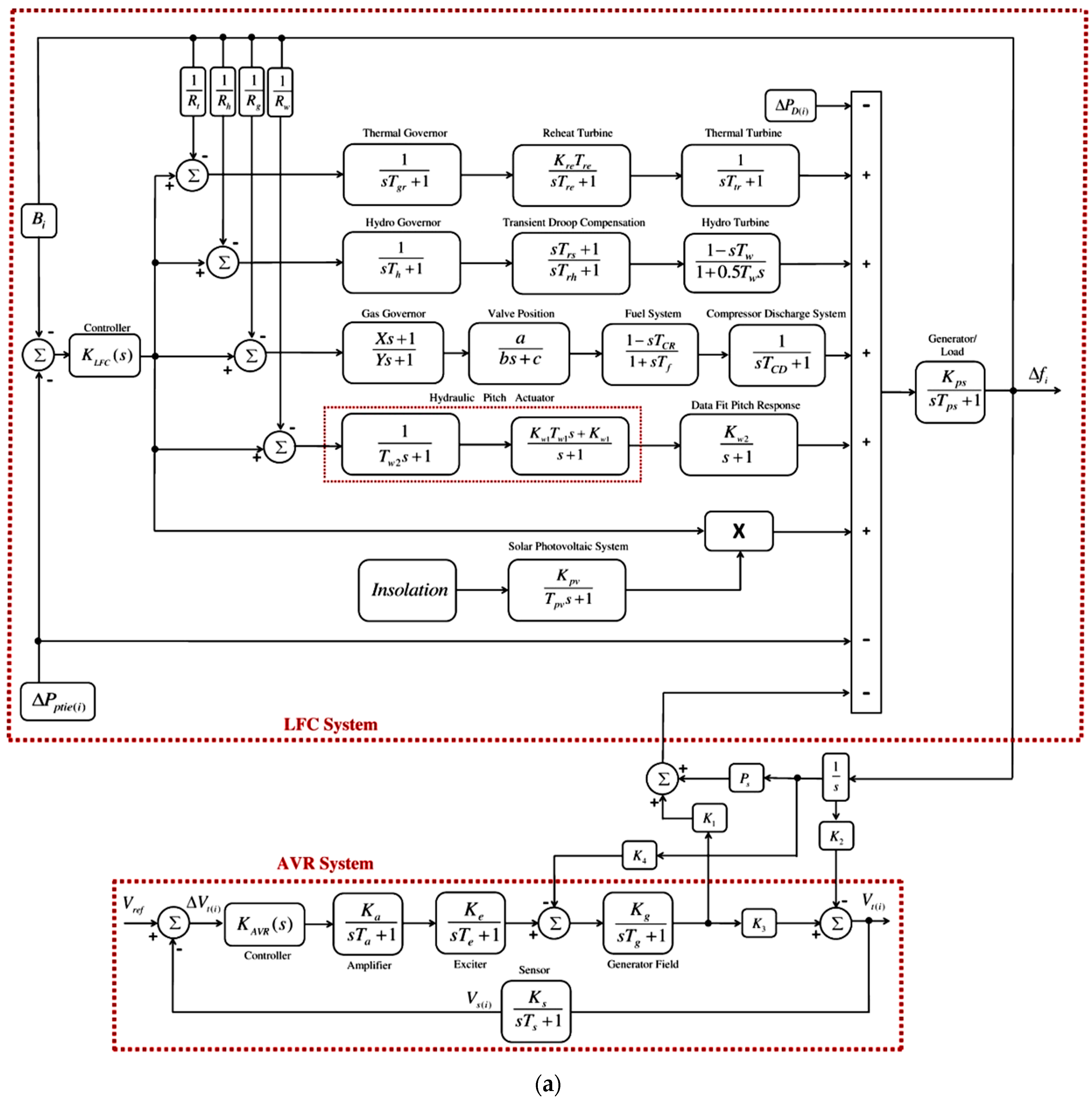
• The mathematical modeling of combined AVR-LFC loops in the proposed four-area IPS, with five generation units, including two renewable energy sources in each area.
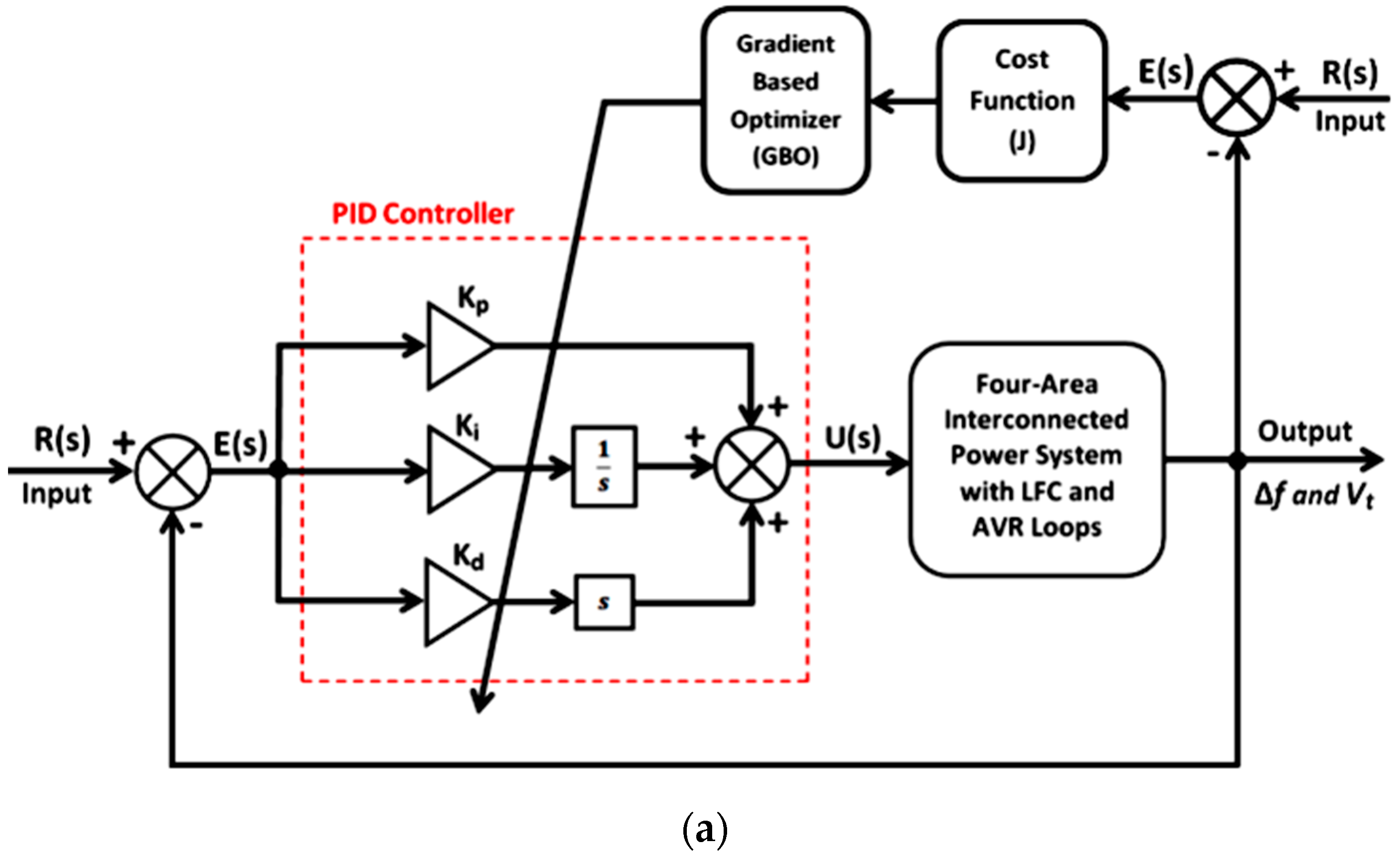
• The mathematical modeling of a proposed PID controller with four-area IPS.
• The formulations of GBO-based fitness functions for the optimal tuning of the PID controller.
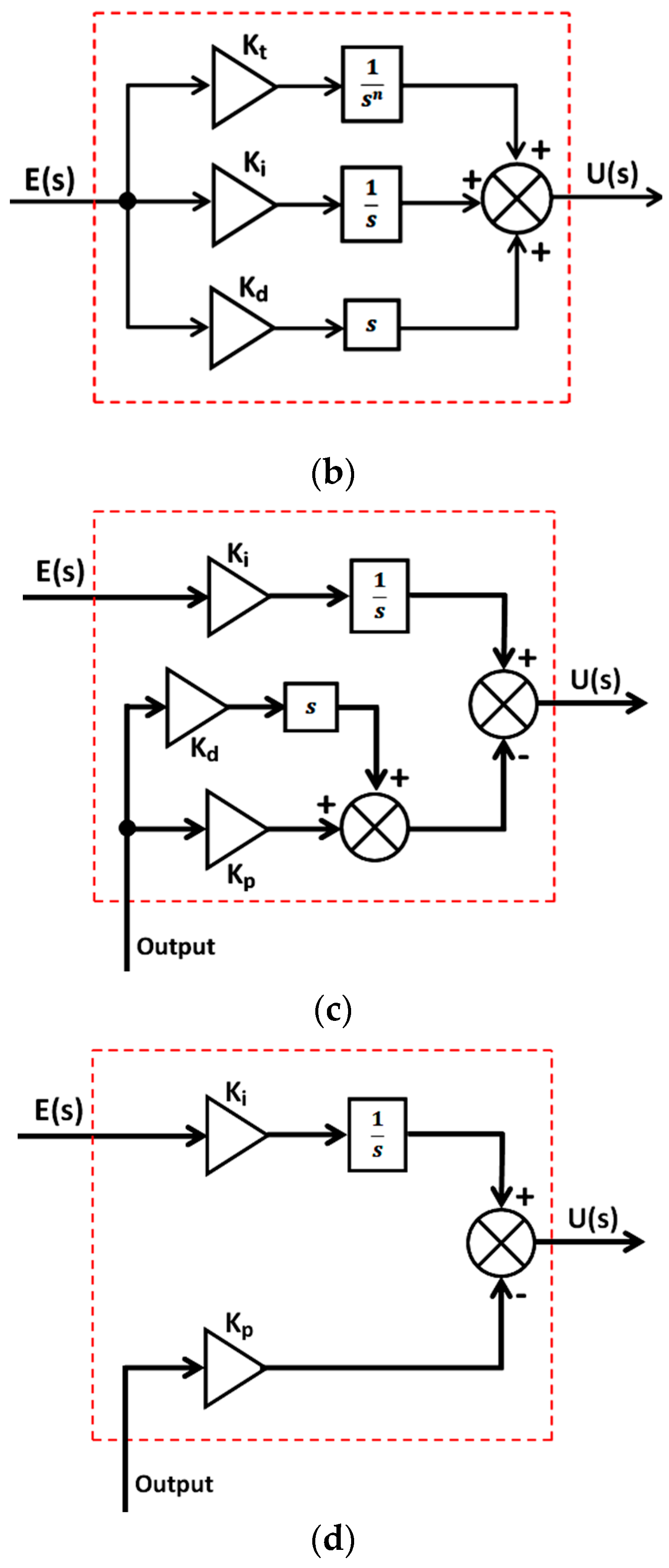
• To evaluate the performance of proposed control methodology, an extensive comparison was made between GBO-PID and other controllers such as GBO-I-PD, GBO-TID, and GBO-I-P in a four-area IPS.
• The robustness of the proposed GBO-PID control methodology was validated by performing a sensitivity analysis by changing the parameters of a four-area IPS over a range of approximately ±25%.

The nomenclature used in this investigation is shown in

Table 2. Acronyms and Notation.

Acronym	Definition	Acronym	Definition
Trh	Transient droop time constant	GBO	Gradient-Based Optimizer
SLP	Step load perturbation	K1, K2, K3, K4,	Cross-coupling coefficients for AVR and LFC loops
PID	Proportional integral derivative	TCR	Combustion reaction time delay
Vt	Terminal voltage	Y	Speed governor lag time constant
I-PD	Integral–proportional derivative	∆f	Frequency deviation
Rt, Rh, Rg, Rw	Speed regulation of thermal reheat, hydro, gas, and wind power plants	T12, T13, T14, T21, T23, T24, T31, T32, T34, T41, T42, T43	Tie-line synchronizing time constants
TID	Tilt integral derivative	Kp	Gain of power system
I-P	Integral–proportional	TCD	Compressor discharge volume time constant
Tp	Time constant of power system	X	Speed governor lead time constant
LFC	Load frequency control	Tw	Water time constant
∆Ptie	Tie-line power deviation	Kw1, Kw2	Wind plant gain constants
AVR	Automatic voltage regulator	Tw1, Tw2	Wind turbine time constants
∆PD	Load deviation	TPV	Solar PV time constant
IPS	Interconnected power system	KPV	Solar PV gain constant
Ttr	Time constant of thermal turbine	a,b,c	Valve positional time constant
B	Area biasing factor	Th	Main servo time constant
Tre	Time constant of reheat steam turbine	Ka	Gain of amplifier
Ta	Time constant of amplifier	Ke	Gain of exciter
Kg	Gain of generator field	Te	Time constant of exciter
Tgr	Time constant of speed governor	Ts	Time constant of voltage sensor
Kre	Gain of reheat steam turbine	Tg	Time constant of generator field
Ks	Gain of voltage sensor	Tf	Fuel time constant
D	Frequency sensitive load coefficient	VS	Sensor voltage
PS	Synchronizing power coefficient	Ve	Error voltage
H	Inertia constant	GDB	Governor dead band
Trs	Speed governor rest time	FTF	Fast traversal filter
GRC	Generation rate constraints	MFO	Moth Flame Optimization
SMES	Superconducting magnetic energy storage	DE	Differential Evolution
NN	Neural network	GWO	Grey Wolf Optimizer
FO	Fractional order	PFA	Pathfinder Algorithm
AOA	Archimedes Optimization Algorithm	NLTA	Nonlinear Threshold Accepting Algorithm
FA	Firefly Algorithm	CFPD	Cascaded Fuzzy PD
IPSO	Improved Particle Swarm Optimization	MPSO	Modified Particle Swarm Optimization
AEFA	Artificial Electric Field Algorithm	AFA	Artificial Flora Algorithm
ADRC	Active disturbance rejection control	UCs	Ultra capacitors
UPFC	Unified Power Flow Controller	CPSS	Conventional power system stabilizer
SCA	Sine Cosine Algorithm	LPBO	Learner Performance-Based Behavior Optimization
FPA	Flower Pollinated Algorithm	IPFC	Interline Power Flow Controller
HHO	Harris Hawks Optimization	DO	Dandelion Optimizer
CTD	Communication time delay	2DOF	Two degrees of freedom
DPO	Doctor and Patient Optimization Technique	ITSE	Integral of time multiplied by squared value of error

. The structure of this research study is as follows: The description of the power system is described in Section 2, and suggested control strategies are discussed in Section 3. An explanation of the proposed GBO algorithm is provided in Section 4. Section 5 presents the simulation work and discussions with all required data. Finally, Section 6 provides conclusions and recommendations for the future.

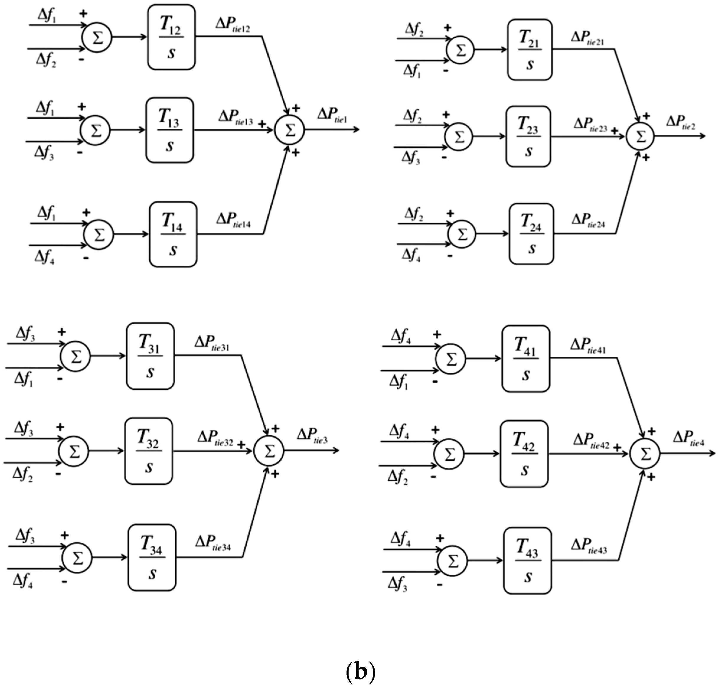
2. Power System Modeling

The four-area multisource IPS model under consideration with integrated AVR and LFC loops is illustrated in Figure 1a. Both loops are cross-coupled using different coupling factors. The IPS consists of four areas, and each area has five sources, namely gas, hydro, reheat thermal units, solar photovoltaic, and wind generation units. Each LFC area is connected to the other area using tie lines, as shown in Figure 1b. The desired frequency of power in an IPS is maintained by an LFC loop. The time constant, gain, and other system parameters of IPS are considered from [10] and listed in Appendix A. The LFC loop of the ith area has gas speed regulation ($R_g$), hydro speed regulation ($R_h$), wind speed regulation ($R_w$), thermal reheat speed regulation ($R_t$), ith area’s bias factor ($B_i$), controller $K_{LFC}(s)$, and generator/load ($\frac{K_{p(i)}}{s{T}_{p(i)}+1}$). The thermal reheat unit consists of a thermal governor ($\frac{1}{s{T}_{gr}+1}$), reheat turbine ($\frac{K_{re}{T}_{re}}{s{T}_{re}+1}$), and thermal turbine ($\frac{1}{s{T}_{tr}+1}$); the hydro unit consists of transient droop compensation ($\frac{s{T}_{rs}+1}{s{T}_{rh}+1}$), hydro governor ($\frac{1}{s{T}_h+1}$), and hydro turbine ($\frac{1-s{T}_w}{1+0.5T_{w}s}$); the gas unit comprises a gas governor ($\frac{Xs+1}{Ys+1}$), valve position ($\frac{a}{bs+c}$), fuel system ($\frac{1-s{T}_{CR}}{1+s{T}_f}$), and compressor discharge system ($\frac{1}{s{T}_{CD}+1}$); the wind unit consists of data fit pitch response and hydraulic pitch actuator blocks; the solar photovoltaic system consists of a straight step function. $\mathsf{\Delta }{P}_{D(i)}$, $\mathsf{\Delta }{P}_{tie(i)}$, $\mathsf{\Delta }{V}_{t(i)}$, and $\mathsf{\Delta }{f}_{(i)}$ denote the deviations in load, tie-line power, terminal voltage, and load frequency, respectively. $V_{s(i)}$, $V_{ref(i)}$, $V_{e(i)}$, and $V_{t(i)}$depict the sensor, reference, error, and terminal voltage in the ith area, respectively. The AVR loop of the ith area comprises an amplifier ($\frac{K_{a(i)}}{s{T}_{a(i)}+1}$), generator ($\frac{K_{g(i)}}{s{T}_{g(i)}+1}$), exciter ($\frac{K_{e(i)}}{s{T}_{e(i)}+1}$), sensor ($\frac{K_{s(i)}}{s{T}_{s(i)}+1}$), and controller ($K_{AVR}(s)$). In order to couple AVR and LFC loops, different coupling coefficients are used, including K₁, K₂, K₃, K₄, and P_s. T_ij denotes the coefficient of synchronization between the ith and ith areas. The transfer function of the gas $(G_G(s))$, reheat thermal $(G_T(s))$, hydro $(G_H(s))$, wind $(G_W(s))$, and solar photovoltaic $(G_S(s))$ systems are provided in Equations (1)–(5), respectively. Table 2 defines the terms used in the LFC and AVR systems.

$$G_G(s)=\frac{(1+Xs)(1-T_{CR}s)a}{(1+Ys)(c+bs)(1+T_{F}s)(1+T_{CD}s)}$$

(1)

$$G_T(s)=\frac{1+T_{re}{K}_{re}s}{(1+T_{gr}s)(1+T_{re}s)(1+T_{tr}s)}$$

(2)

$$G_H(s)=\frac{(1+T_{rs}s)(1-T_{w}s)}{(1+T_{h}s)(1+T_{rh}s)(1+0.5T_{w}s)}$$

(3)

$$G_W(s)=\frac{K_{w1}{K}_{w2}(1+T_{w1}s)}{(1+T_{w2}s)(s^2+2s+1)}$$

(4)

$$G_S(s)=\frac{K_{pv}}{1+T_{pv}}$$

(5)

The AVR is responsible for regulating the voltage of the synchronous generator to a specific value. By continuously comparing the output voltage with the reference signal, the error voltage is determined. The error signal is amplified before it is fed to the exciter to change the excitation of the generator field. This procedure immediately corrects the terminal voltage fluctuation and stabilizes the system.

3. Proposed Control Methodology

Figure 2a demonstrates the proposed methodology with IPS. A PID controller was employed for the combined LFC and AVR control of the four-area IPS. Further, various other controllers such as I-PD, TID, and I-P have also been explored to compare their results with GBO-PID. The description of the proposed PID and the other controllers is provided in this section.

The traditional PID controller is utilized extensively in the industrial sector due to its inherited characteristics of simple design and excellent operational efficiency. The proportional integral derivative (PID) controller is a feedback-based control loop system that generates the control signal for the plant by continually calculating an error signal as the difference between the set point and a measured process variable. The PID controller has three gain coefficients, K_p, K_i, and K_d. The control signal generated by PID controller (U_PID(s)) can be written as:

$$U_{PID}(s)=(K_p+\frac{K_i}{s}+K_{d}s)E(s)$$

(6)

$$E(s)=Y(s)-R(s)$$

(7)

where, E(s), Y(s), and R(s) denote error, output, and reference signals, respectively. The TID controller’s architecture is identical to PID but with a modification in the proportional term of PID. The change is that PID’s proportional gain term is replaced by K_t (s)^−1/n, where n is a real number and K_t represents the gain. TID combines integer and fractional order controllers. It quickly eliminates disturbances due to its superior dynamic features. Figure 2b shows the block diagram of the TID controller. The TID controller has three gain coefficients: K_t, K_i, and K_d. The control signal generated by the TID controller (U_TID(s)) can be written as:

$$U_{TID}(s)=(K_t{s}^{-\frac{1}{n}}+\frac{K_i}{s}+K_{d}s)E(s)$$

(8)

The I-PD controller has the capacity to improve the controller’s transient responsiveness, in particular the overshoot time. The proportional and derivative terms are placed in the feedback path of the I-PD controller, whereas the integrator controller is placed in the feed-forward direction. Figure 2c shows the block diagram of the I-PD controller. The I-PD controller has three gain coefficients: K_i, K_p, and K_d. The control signal generated by the I-PD controller (U_I-PD(s)) can be written as:

$$U_{I-PD}(s)=\frac{K_i}{s}E(s)-(K_p+K_{d}s)Y(s)$$

(9)

In an I-P controller, only the proportional term is placed in the feedback path whereas the integrator controller is placed in the feed-forward direction. Figure 2d shows the block diagram of the I-P controller. The I-P controller has two gain coefficients: K_i and K_p. The control signal generated by the I-P controller (U_I-P(s)) can be written as:

$$U_{I-P}(s)=\frac{K_i}{s}E(s)-K_{p}Y(s)$$

(10)

The optimal gains of controllers, as highlighted in Equations (6) and (8)–(10), are obtained using the gradient-based optimizer (GBO) that is described in the next section. Further, ITSE [1] has been used as an error specification index for the optimal control of LFC and AVR loops in the four-area IPS using GBO-PID control methodology. The cost function (J) for the four-area IPS is obtained using Equation (11).

$${\mathrm{J}}_{\mathrm{ITSE}}={\int }_0^{T}t[\mathsf{\Delta }{f}^2+\mathsf{\Delta }{V}_t^2+\mathsf{\Delta }{P}_{tie}^2]dt$$

(11)

where

$$\begin{array}{c}\mathsf{\Delta }{f}^2=\mathsf{\Delta }{f}_1^2+\mathsf{\Delta }{f}_2^2+\mathsf{\Delta }{f}_3^2+\mathsf{\Delta }{f}_4^2\\ \mathsf{\Delta }{V}_t^2=\mathsf{\Delta }{V}_{t1}^2+\mathsf{\Delta }{V}_{t2}^2+\mathsf{\Delta }{V}_{t3}^2+\mathsf{\Delta }{V}_{t4}^2\\ \mathsf{\Delta }{P}_{tie}^2=\mathsf{\Delta }{P}_{tie1}^2+\mathsf{\Delta }{P}_{tie2}^2+\mathsf{\Delta }{P}_{tie3}^2+\mathsf{\Delta }{P}_{tie4}^2\end{array}$$

(12)

$$\begin{array}{c}\mathsf{\Delta }{V}_{t1}=V_{ref}-V_{t1}\\ \mathsf{\Delta }{V}_{t2}=V_{ref}-V_{t2}\\ \mathsf{\Delta }{V}_{t3}=V_{ref}-V_{t3}\\ \mathsf{\Delta }{V}_{t4}=V_{ref}-V_{t4}\end{array}$$

(13)

$$\begin{array}{c}\mathsf{\Delta }{P}_{ptie1}=\mathsf{\Delta }{P}_{ptie12}+\mathsf{\Delta }{P}_{ptie13}+\mathsf{\Delta }{P}_{ptie14}\\ \mathsf{\Delta }{P}_{ptie2}=\mathsf{\Delta }{P}_{ptie21}+\mathsf{\Delta }{P}_{ptie23}+\mathsf{\Delta }{P}_{ptie24}\\ \mathsf{\Delta }{P}_{ptie3}=\mathsf{\Delta }{P}_{ptie31}+\mathsf{\Delta }{P}_{ptie32}+\mathsf{\Delta }{P}_{ptie34}\\ \mathsf{\Delta }{P}_{ptie4}=\mathsf{\Delta }{P}_{ptie41}+\mathsf{\Delta }{P}_{ptie42}+\mathsf{\Delta }{P}_{ptie43}\end{array}$$

(14)

The cost function given by Equation (11) is minimized using GBO to yield the optimal gains of the controller.

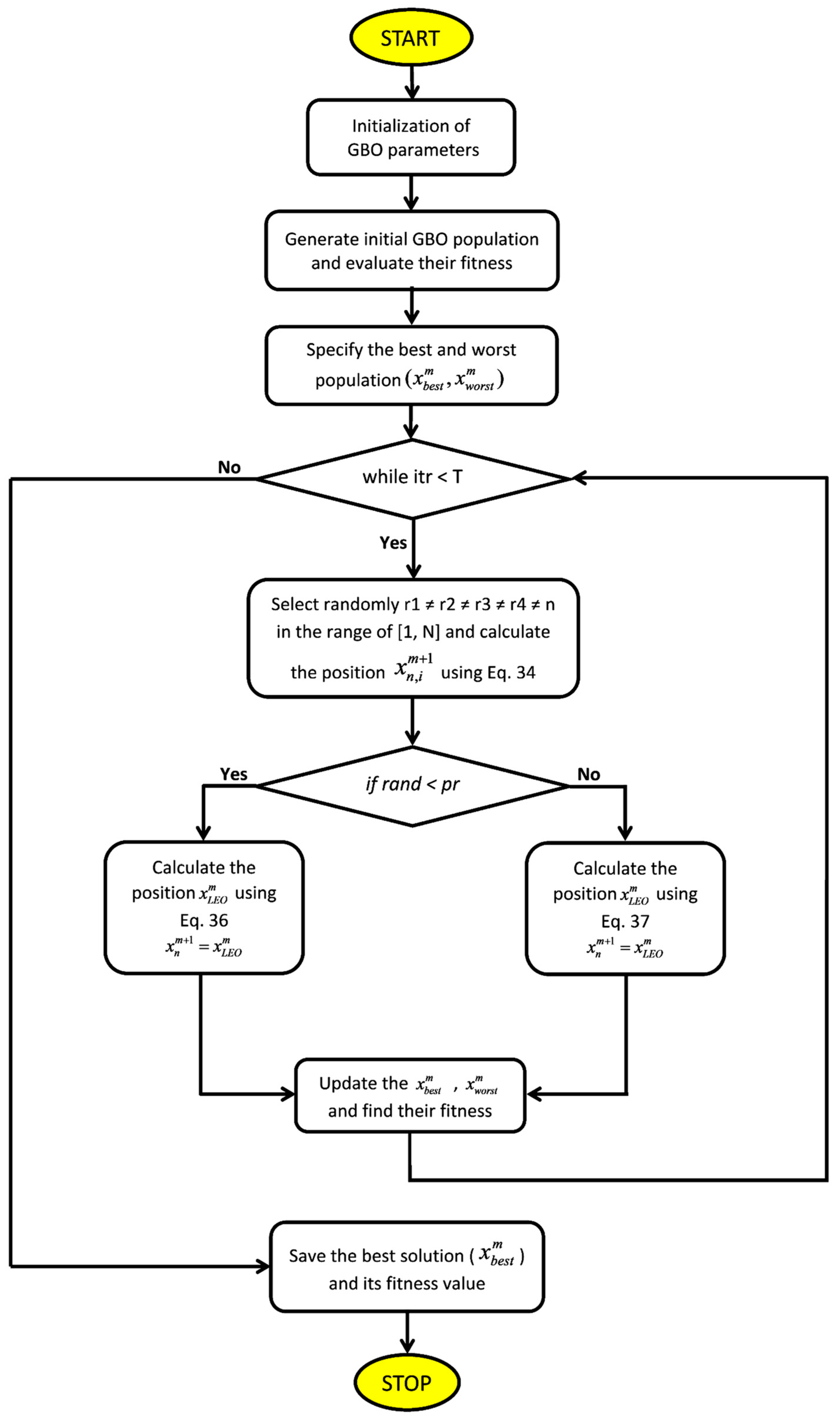
4. Gradient-Based Optimizer (GBO)

The four-area power system with five generation units is a very complex system that presents a very challenging task for the control system engineers to design a controller capable of maintaining terminal voltage and load frequency within prescribed limits. Nature-inspired computation algorithms that are capable of handling complex engineering problems have attracted much attention in the control of IPSs. In this study, load frequency and the terminal voltage of a four-area IPS were successfully regulated using a PID controller tuned with a gradient-based optimizer (GBO). The significance of the GBO algorithm in automatic voltage control applications motivated the authors to explore it for combined control of load frequency and terminal voltage [34]. GBO-based control methods provided satisfactory time responses in terms of settling time, % overshoot, and % undershoot. GBO was developed by Iman Ahmadianfar et al. in 2020 [43]. The GBO algorithm is inspired by Newton’s gradient-based method; it uses a range of vectors to seek the problem’s solution space. This search is carried out using mutational methods such as local escaping and gradient search rules. It is necessary to locate an equilibrium point where the slope is zero so that this algorithm can identify the best solution. With this approach, finding the search directions requires figuring out the objective function’s derivatives in conjunction with constraints. The initial population is produced at random, and the information from previous iterations is used to determine a search direction. These cycles are repeated until a particular need is satisfied. The steps in a gradient-based optimizer (GBO) are as follows [44].

A.

GBO INITIALIZATION

The GBO population is initialized as follows:

$$X_n=X_{\min }+rand(0,1)\times (X_{\max }-X_{\min })$$

(15)

$$X_{n,d}=[X_{n,1},X_{n,2},\dots ,X_{n,D}]$$

(16)

where n = [1,2,… ,N] represents the population trajectories; d = [1,2,…..,D] denotes the search space dimensions; rand (0,1) generates a uniform random number between 0 and 1; and X_min and X_max are the limits of the decision variable.

B.

GRADIENT SEARCH RULE (GSR)

The gradient-based technique, which forms the basis of GSR, finds the optimal solution by identifying the extreme point at which the gradient equals zero. The objectives of employing GSR include acceleration of convergence rate and exploration tendency enhancement. The numerical gradient approach and Taylor series can be used to express a new position ($x_{n+1}$):

$$x_{n+1}=x_n-\frac{2\mathsf{\Delta }x\times f(x_n)}{f(x_n+\mathsf{\Delta }x)-f(x_n-\mathsf{\Delta }x)}$$

(17)

In the GBO algorithm, $x_n+\mathsf{\Delta }x$ and $x_n-\mathsf{\Delta }x$ represent the neighboring positions of $x_n$. The position $x_n+\mathsf{\Delta }x$ has a worse fitness ($x_{worst}$) than $x_n$, while $x_n-\mathsf{\Delta }x$ has better fitness ($x_{best}$) than $x_n$. The GSR can be written as:

$$GSR=randn\times \frac{2\mathsf{\Delta }x\times x_n}{(x_{worst}-x_{best}+\epsilon )}$$

(18)

where ∆x is the change in position after each iteration, ε is a small value between 0 and 0.1, and randn denotes a random number from a normal distribution. In order to achieve a balance between the exploitation and exploration phases, the modified expression of GSR can be stated as:

$$GSR=randn\times {\rho }_1\times \frac{2\mathsf{\Delta }x\times x_n}{(x_{worst}-x_{best}+\epsilon )}$$

(19)

where ${\rho }_1$ is a random number computed as:

$${\rho }_1=(2\times rand\times \alpha )-\alpha$$

(20)

$$\alpha =\left|\beta \times \sin \left(\frac{3\pi }{2}+\sin \left(\beta \times \frac{3\pi }{2}\right)\right)\right|$$

(21)

$$\beta ={\beta }_{\min }+({\beta }_{\max }-{\beta }_{\min })\times {\left(1-{\left(\frac{m}{M}\right)}^3\right)}^2$$

(22)

where M represents total number of iterations, m shows current iteration, and β_max and β_min have values of 1.2 and 0.2, respectively. The sine function representing the change from exploration to exploitation is represented by $\alpha$. The difference ∆x between the best candidate solution ($x_{best}$) and a position chosen at random ($x_{r1}^m$) can be written as:

$$\mathsf{\Delta }x=rand(1:N)\times \left|step\right|$$

(23)

$$step=\frac{(x_{best}-x_{r1}^m)+\delta }{2}$$

(24)

$$\delta =2\times rand\times \left(\left|\frac{x_{r1}^m+x_{r2}^m+x_{r3}^m+x_{r4}^m}{4}-x_n^m\right|\right)$$

(25)

where r1, r2, r3, and r4 are random numbers between 1 and N having different values. The updated position ($x_{n+1}$) can be expressed as:

$$x_{n+1}=x_n-GSR$$

(26)

For better utilization of the region close to$x_n$, the direction of movement (DM) is introduced and can be written as:

$$DM=rand\times {\rho }_2\times (x_{best}-x_n)$$

(27)

where ρ₂ is a random number computed as:

$${\rho }_2=(2\times rand\times \alpha )-\alpha$$

(28)

The modified position (${X1}_n^m$) can be found using GSR and DM as:

$${X1}_n^m=x_n^m-GSR+DM$$

(29)

$${X1}_n^m=x_n^m-randn\times {\rho }_1\times \frac{2\mathsf{\Delta }x\times x_n^m}{(x_{worst}-x_{best}+\epsilon )}$$

(30)

The new vector (${X2}_n^m$) can be created by replacing the position of the best vector ($x_{best}$) with $x_n^m$.

$${X2}_n^m=x_{best}-randn\times {\rho }_1\times \frac{2\mathsf{\Delta }x\times x_n^m}{(y{p}_n^m-y{q}_n^m+\epsilon )}+rand\times {\rho }_2\times (x_{r1}^m-x_{r2}^m)$$

(31)

where

$$y{p}_n=rand\times \left(\frac{[z_{n+1}+x_n]}{2}+rand\times \mathsf{\Delta }x\right)$$

(32)

$$y{q}_n=rand\times \left(\frac{[z_{n+1}+x_n]}{2}-rand\times \mathsf{\Delta }x\right)$$

(33)

and $z_{n+1}$represents a vector.

The new solution ($x_n^{m+1}$) can be defined at the next iteration as:

$$x_n^{m+1}=r_a\times (r_b\times {X1}_n^m+(1-r_b)\times {X2}_n^m)+(1-r_a)\times {X3}_n^m$$

(34)

where

$${X3}_n^m=X_n^m-{\rho }_1\times ({X2}_n^m-{X1}_n^m)$$

(35)

and r_a and r_b are random numbers between 0 and 1.

C.

LOCAL ESCAPING OPERATOR (LEO)

To improve the GBO algorithm’s capability to handle challenging problems, a LEO is included. The LEO solution ($X_{LEO}^m$) can be obtained by using the following pseudo code:

$$\begin{array}{l}ifrand<pr\\ ifrand<0.5\\ X_{LEO}^m=X_n^{m+1}+f_1\times (u_1\times x_{best}-u_2\times x_k^m)+f_2\times {\rho }_1\times (u_3\times (X{2}_n^m-X{1}_n^m)+u_2\times (x_{r1}^m-x_{r2}^m))/2\\ X_n^{m+1}=X_{LEO}^m\end{array}$$

(36)

$$\begin{array}{l}else\\ X_{LEO}^m=x_{best}+f_1\times (u_1\times x_{best}-u_2\times x_k^m)+f_2\times {\rho }_1\times (u_3\times (X{2}_n^m-X{1}_n^m)+u_2\times (x_{r1}^m-x_{r2}^m))/2\\ X_n^{m+1}=X_{LEO}^m\\ end\\ end\end{array}$$

(37)

where $x_{best}$ shows the best solution; $x_{r1}^m$, $x_{r2}^m$, and $x_k^m$ are randomly generated solutions; f₂ is a random number with a standard deviation of 1 and mean of 0 whereas f₁ is a random number between −1 and 1; pr represents the probability; and u₁, u₂, and u₃ can be obtained as:

$$u_1=L_1\times 2\times rand+(1-L_1)$$

(38)

$$u_2=L_1\times rand+(1-L_1)$$

(39)

$$u_3=L_1\times 2\times rand+(1-L_1)$$

(40)

where L₁ has a value of 1 if parameter u₁ is less than 0.5, otherwise it has a value of 0; $x_k^m$can be written as:

$$x_k^m=\{\begin{array}{ll}{x}_{rand}& \mathrm{if} u_2<0.5\\ x_p^m& \mathrm{otherwise}\end{array}$$

(41)

where $x_{rand}$ represents the new solution and $x_p^m$ denotes random solution of the population (P ∈ [1,2,…,N]).

$$x_{rand}=X_{\min }+rand(0,1)\times (X_{\max }-X_{\min })$$

(42)

$$x_k^m=L_2\times x_p^m+(1-L_2)\times x_{rand}$$

(43)

where L₂ has a value of 1 if parameter u₂ is less than 0.5, otherwise it has a value of 0. By choosing values for the parameters u₁, u₂, and u₃ randomly, the population becomes more diverse and is able to avoid local optimal solutions. The flow chart of GBO is given in Figure 3.

5. Simulations and Discussion of Results

Extensive simulations were conducted in MATLAB/Simulink to validate the suggested control methodology. The rated power of the system is considered as 2000 MW and the models of generation units have been taken from [10]. First, a four-area, five-source IPS with 5% SLP (0.05 p.u.) in each area was comprehensively examined using GBO-based control methodologies. Then, by changing the system settings in each of the four areas, a detailed sensitivity analysis was carried out. The population consists of thirty solutions whereas twenty iterations were considered in each simulation to obtain the optimal solution. The step input per unit was taken as reference terminal voltage. Recall that ±2% tolerance was considered to obtain the settling time in each simulation.

A.

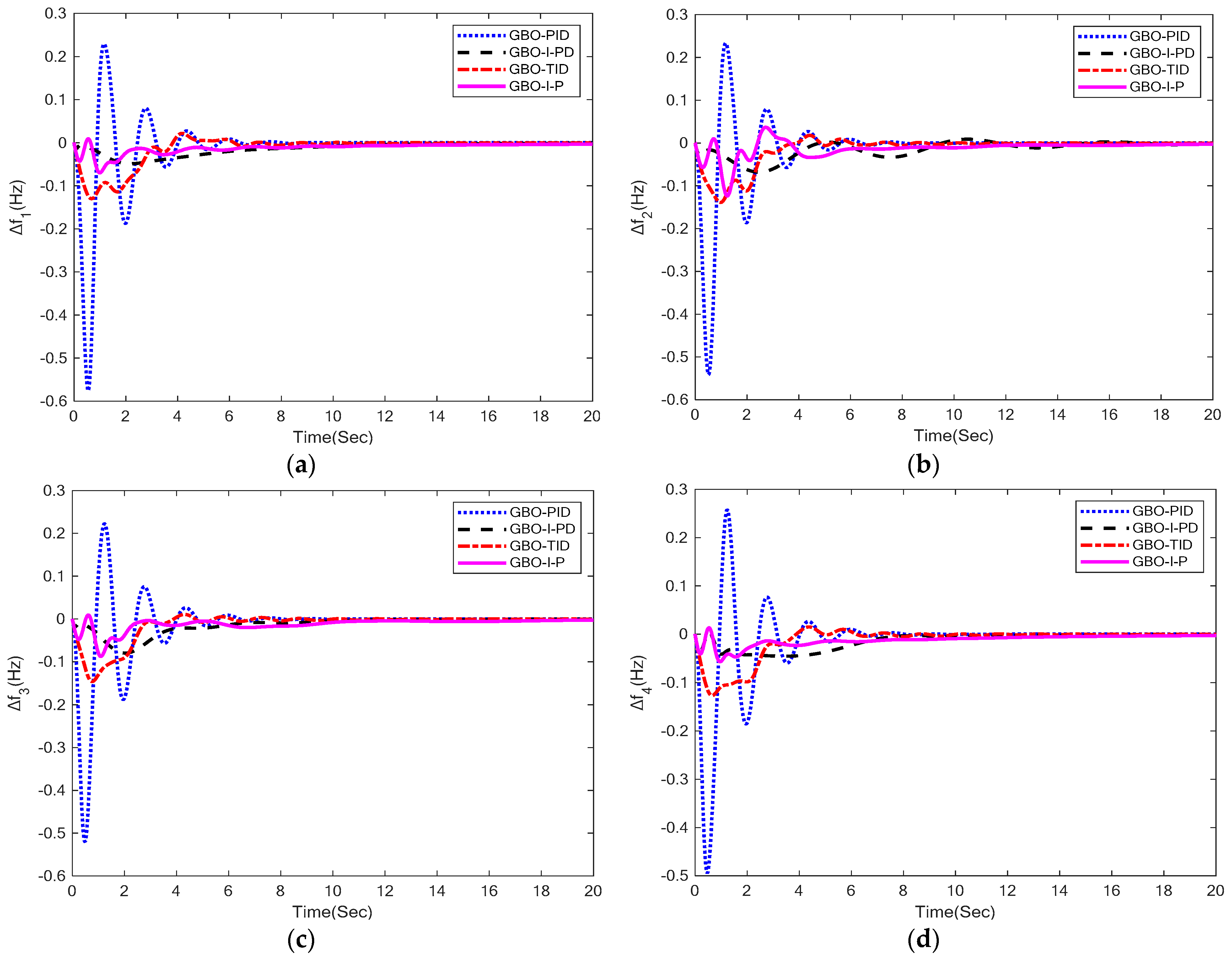
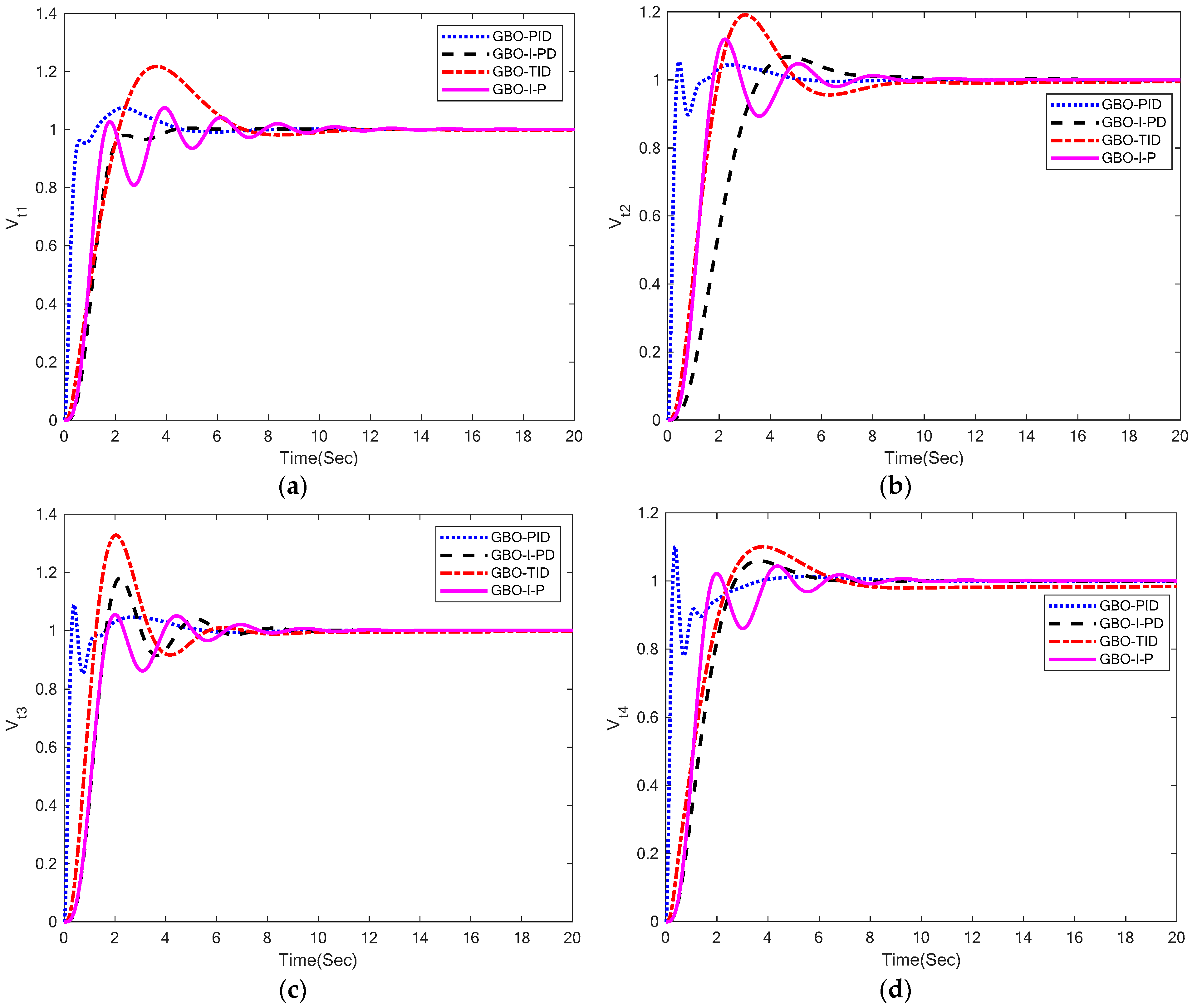
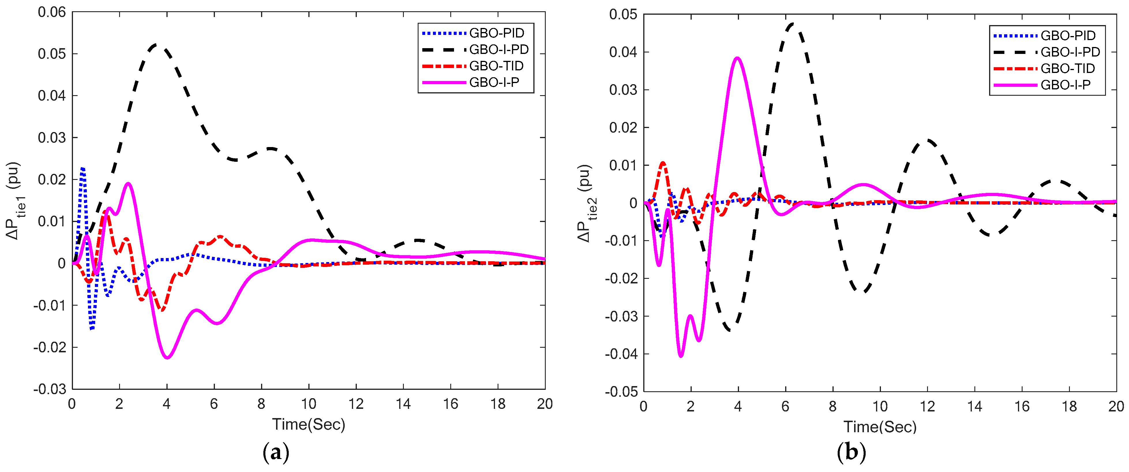
FOUR-AREA IPS WITH COMBINED AVR-LFC

The four-area IPS model under investigation is shown in Figure 1. The system parameters of the four-area IPS are given in Appendix A. The optimal parameters of GBO-PID, GBO-I-PD, GBO-TID, and GBO-I-P control methodologies are given in

Table 3. Optimum controller parameters.

Area	GBO−I-P		GBO−TID		GBO−I−PD		GBO−PID
	Controller Parameter	Value	Controller Parameter	Value	Controller Parameter	Value	Controller Parameter	Value
Area−1	Kp1	0.17	Kt1	0.76	Ki1	0.0001	Kp1	1.43
	Ki1	2.42	Ki1	1.29	Kp1	1.59	Ki1	1.27
	-	-	Kd1	0.20	Kd1	1.97	Kd1	1.93
	Kp2	1.37	Kt2	0.97	Ki2	1.09	Kp2	1.08
	Ki2	1.38	Ki2	0.29	Kp2	1.15	Ki2	1.11
	-	-	Kd2	1.18	Kd2	0.15	Kd2	0.67
Area−2	Kp3	1.43	Kt3	1.54	Ki3	0.74	Kp3	1.11
	Ki3	0.82	Ki3	1.27	Kp3	0.25	Ki3	1
	-	-	Kd3	0.30	Kd3	0.54	Kd3	1.24
	Kp4	0.92	Kt4	0.44	Ki4	0.35	Kp4	1.37
	Ki4	0.83	Ki4	0.18	Kp4	0.41	Ki4	1.20
	-	-	Kd4	0.20	Kd4	0.14	Kd4	0.96
Area−3	Kp5	1.15	Kt5	1.82	Ki5	0.01	Kp5	1.74
	Ki5	1.67	Ki5	0.42	Kp5	0.65	Ki5	1.76
	-	-	Kd5	1.73	Kd5	1.28	Kd5	0.99
	Kp6	1.11	Kt6	0.87	Ki6	1.06	Kp6	1.33
	Ki6	1.09	Ki6	0.31	Kp6	0.85	Ki6	1.27
	-	-	Kt6	0.24	Kd6	0.047	Kd6	1.13
Area−4	Kp7	0.12	Kt7	1.78	Ki7	0.99	Kp7	0.98
	Ki7	2.78	Ki7	0.28	Kp7	2	Ki7	1.94
	-	-	Kd7	0.62	Kd7	0.14	Kd7	1.39
	Kp8	1.10	Kt8	1.30	Ki8	1.15	Kp8	1.24
	Ki8	1.13	Ki8	0.069	Kp8	1.28	Ki8	0.61
	-	-	Kd8	1.50	Kd8	0.58	Kd8	1.26
	ITSE	2.18	ITSE	2.62	ITSE	3.43	ITSE	0.71

. This section presents a detailed comparison of the proposed GBO-PID, GBO-I-PD, GBO-TID, and GBO-I-P control methodologies. Figure 4 displays the frequency deviation response curves, while

Table 4. Numerical results of LFC loops.

Control Strategy	Area-1				Area-2
	Settling Time	% Overshoot	% Undershoot	% s-s Error	Settling Time	% Overshoot	% Undershoot	% s-s Error
GBO-PID	5.37	0.23	−0.58	0	5.38	0.23	−0.54	0
GBO-I-PD	16.3	0	−0.049	0	19.54	0.009	−0.068	0
GBO-TID	9.66	0.022	−0.13	0	9.51	0.018	−0.14	0
GBO-I-P	16.10	0.0086	−0.07	0	16.49	0.036	−0.12	0
Control Strategy	Area-3				Area-4
	Settling Time	% Overshoot	% Undershoot	% s-s Error	Settling Time	% Overshoot	% Undershoot	% s-s Error
GBO-PID	5.38	0.22	−0.52	0	5.98	0.26	−0.49	0
GBO-I-PD	11.0	0	−0.08	0	17.08	0.0039	−0.046	0
GBO-TID	9.62	0.011	−0.15	0	9.68	0.015	−0.13	0
GBO-I-P	17.66	0.009	−0.087	0	16.95	0.013	−0.057	0

presents the numerical results of LFC performance specifications for each of the four areas utilizing the GBO-PID, GBO-I-PD, GBO-TID, and GBO-I-P control methodologies. It can be observed that the proposed GBO-PID control strategy delivered highly satisfactory LFC responses in terms of settling time in each area. GBO-PID provided settling times of 5.37, 5.38, 5.38, and 5.98 s in area-1, area-2, area-3, and area-4 LFC, respectively, which are better than GBO-I-PD, GBO-TID, and GBO-I-P control methodologies at the cost of percent (%) overshoot and undershoot in each area. GBO-I-PD yielded better undershoot response (−0.049) with zero % overshoot compared to other control methodologies in area-1 LFC. In comparison to other control methodologies in area-2 LFC, GBO-I-PD provided better % overshoot (0.009%) and undershoot (−0.068) responses. In area-3 LFC, GBO-I-PD produced a better undershoot response (−0.08) with zero % overshoot when compared to other control methods. GBO-I-PD yielded better % overshoot (0.0039%) and undershoot response (−0.046) compared to other control methodologies in area-4 LFC. The steady-state error is zero with all control methodologies in each area.

Figure 5 displays the terminal voltage response curves, while

Table 5. Numerical results for AVR loops.

Control Strategy	Area-1			Area-2
	Settling Time	% Overshoot	% s-s Error	Settling Time	% Overshoot	% s-s Error
GBO-PID	3.96	7.52	0	4.09	5.45	0
GBO-I-PD	3.72	0.48	0	6.75	6.66	0
GBO-TID	6.60	21.91	0	7.68	19.71	1.8
GBO-I-P	7.52	7.43	0	5.68	11.9	0
Control Strategy	Area-3			Area-4
	Settling Time	% Overshoot	% s-s	Settling Time	% Overshoot	% s-s
			Error			Error
GBO-PID	4.36	9.0	0	2.92	10.13	0
GBO-I-PD	5.72	18.04	0	5.27	5.90	0
GBO-TID	5.24	33.18	0	6.72	11.90	0
GBO-I-P	7.01	5.52	0	5.92	4.36	0

presents the numerical results of AVR performance specifications obtained in area 1, 2, 3, and 4 utilizing the GBO-PID, GBO-I-PD, GBO-TID, and GBO-I-P control methodologies, respectively. For area-1 AVR, GBO-PID provided a settling time of 3.96 s that is quicker than GBO-TID and GBO-I-P control methodologies. Moreover, GBO-PID yielded settling times of 4.09, 4.36, and 2.92 in area-2, area-3, and area-4 AVR, which are better than GBO-I-PD, GBO-TID, and GBO-I-P control methodologies. GBO-I-PD produced a settling time of 3.72 s with 0.48% overshoot response, which is better than all other control methodologies in area-1 AVR. GBO-PID yielded an overshoot of 5.45% in area-2 AVR, which is better than GBO-I-PD, GBO-TID, and GBO-I-P control methodologies. GBO-PID produced an overshoot of 9%, which is better than GBO-I-PD and GBO-TID control methodologies in area-3 AVR. GBO-I-P outperformed all other techniques in area-3 AVR by 5.52% in terms of overshoot response. GBO-PID provided 10.13% overshoot, which is better than GBO-TID control methodology in area-4 AVR. GBO-I-P yielded 4.36% overshoot that is better compared to all other techniques. The steady-state error is zero with all control methodologies, including GBO-PID in each area except GBO-TID, which gave a steady-state error of 1.8% in area-2 AVR. It can be seen that the suggested GBO-PID control technique produced AVR responses that are very satisfactory in terms of settling time and % overshoot.

The tie-line power deviation responses are shown in Figure 6, while the numerical results of tie-line power’s performance specifications for area 1, 2, 3, and 4 are presented in

Table 6. Numerical results of tie-line power deviations.

Control Strategy	Area-1				Area-2
	Settling Time	% Overshoot	% Undershoot	% s-s Error	Settling Time	% Overshoot	% Undershoot	% s-s Error
GBO-PID	9.36	0.023	−0.016	0	9.69	0.0025	−0.0093	0
GBO-I-PD	16.65	0.052	−0.0035	0.004	19.48	0.047	−0.034	0
GBO-TID	11.18	0.012	−0.0112	0	11.02	0.011	−0.0053	0
GBO-I-P	19.50	0.019	−0.023	0	16.12	0.039	−0.040	0
Control Strategy	Area-3				Area-4
	Settling Time	% Overshoot	% Undershoot	% s-s Error	Settling Time	% Overshoot	% Undershoot	% s-s Error
GBO-PID	8.45	0.013	−0.012	0	10.23	0.015	−0.013	0
GBO-I-PD	18.71	0.0038	−0.066	0.004	19.47	0.043	−0.035	0
GBO-TID	9.7	0.015	−0.017	0	9.63	0.0098	−0.0081	0
GBO-I-P	19.17	0.022	−0.015	0	18.23	0.031	−0.007	0

. It can be seen that the suggested GBO-PID control technique produced tie-line power deviation responses that were incredibly satisfactory in terms of settling time in each area. GBO-PID provided settling times of 9.36, 9.69, and 8.45 s in area-1, area-2, and area-3, respectively, which are better than GBO-I-PD, GBO-TID, and GBO-I-P control methodologies. GBO-TID produced a 9.63 s settling time in area-4, which is better than all other control methodologies. GBO-TID yielded a better overshoot (0.012%) response whereas GBO-I-PD produced a better undershoot response (−0.0035) compared to other control methodologies in terms of area-1 tie-line power deviation. GBO-PID yielded 0.0025% overshoot with −0.0093 undershoot, which is better than GBO-I-PD and GBO-I-P control methodologies in terms of area-2 tie-line power deviation. Moreover, GBO-TID yielded a better undershoot response (−0.0053) compared to other control methodologies in terms of area-2 tie-line power deviation. GBO-I-PD produced a better overshoot response (0.0038) whereas GBO-PID yielded a better undershoot response (−0.012) compared to other control methodologies in terms of area-3 tie-line power deviation. GBO-TID yielded a better overshoot response (0.0098) whereas GBO-I-P yielded a better undershoot response (−0.007) compared to other control methodologies in terms of area-4 tie-line power deviation. The steady-state error is zero with each control methodology except GBO-I-PD, which produced negligible steady state in area-1 and area-3.

B.

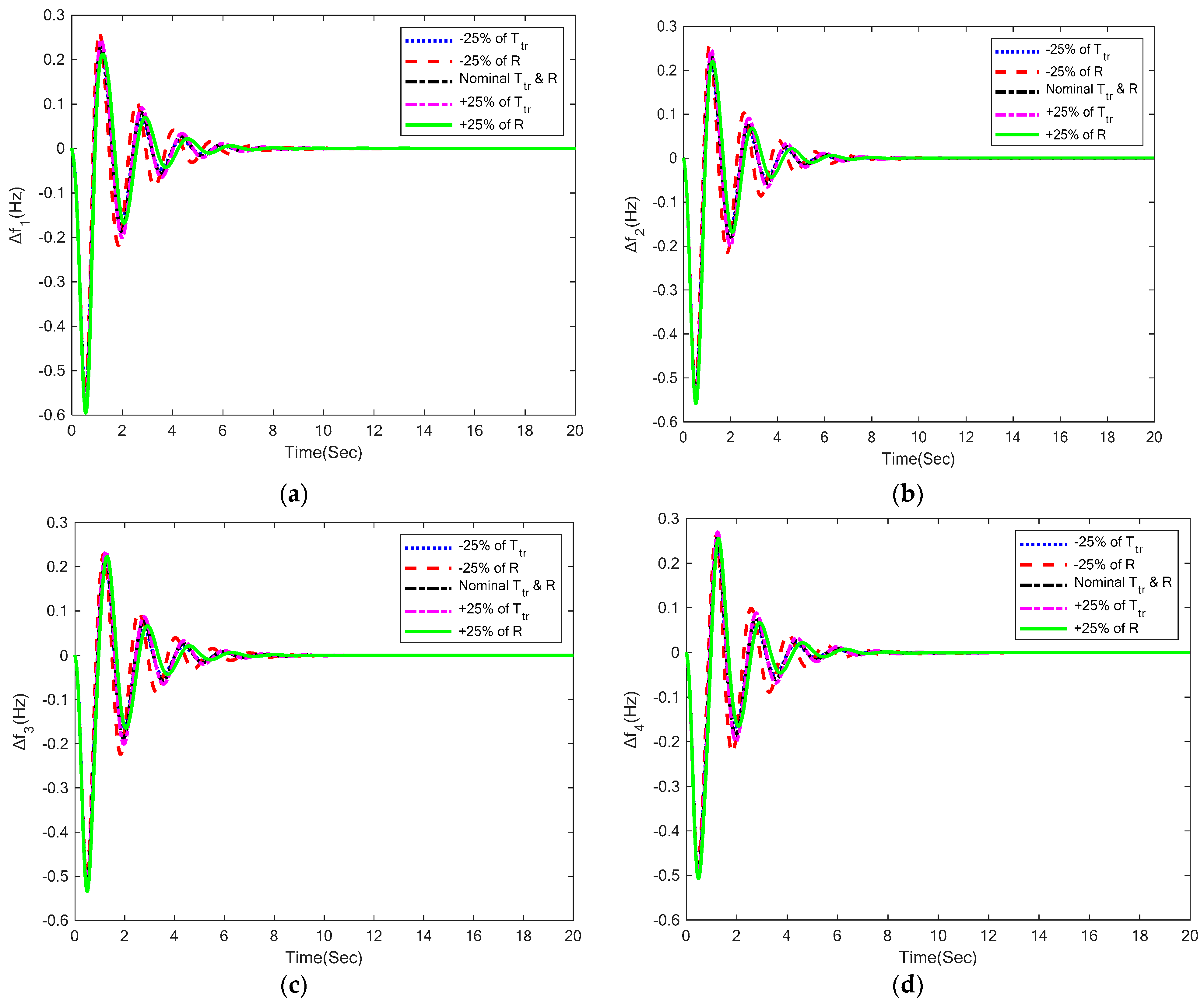
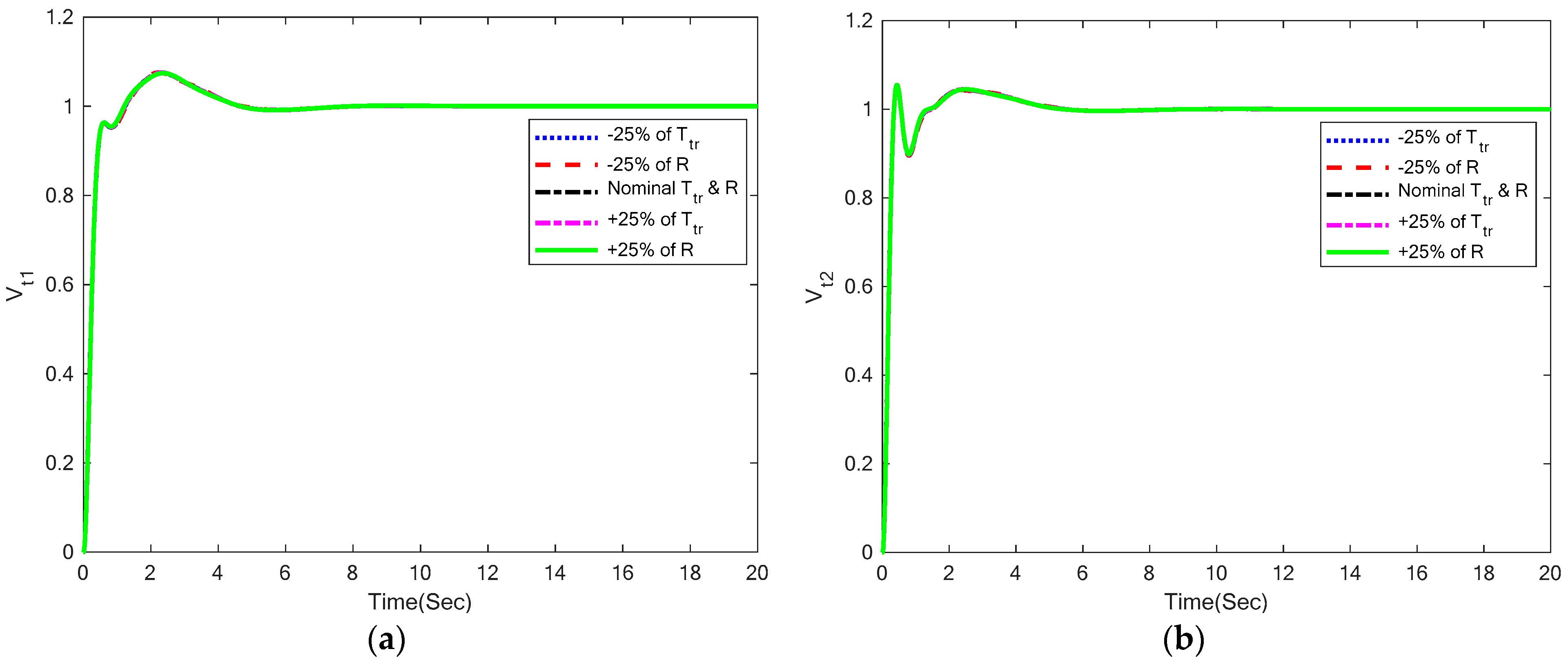
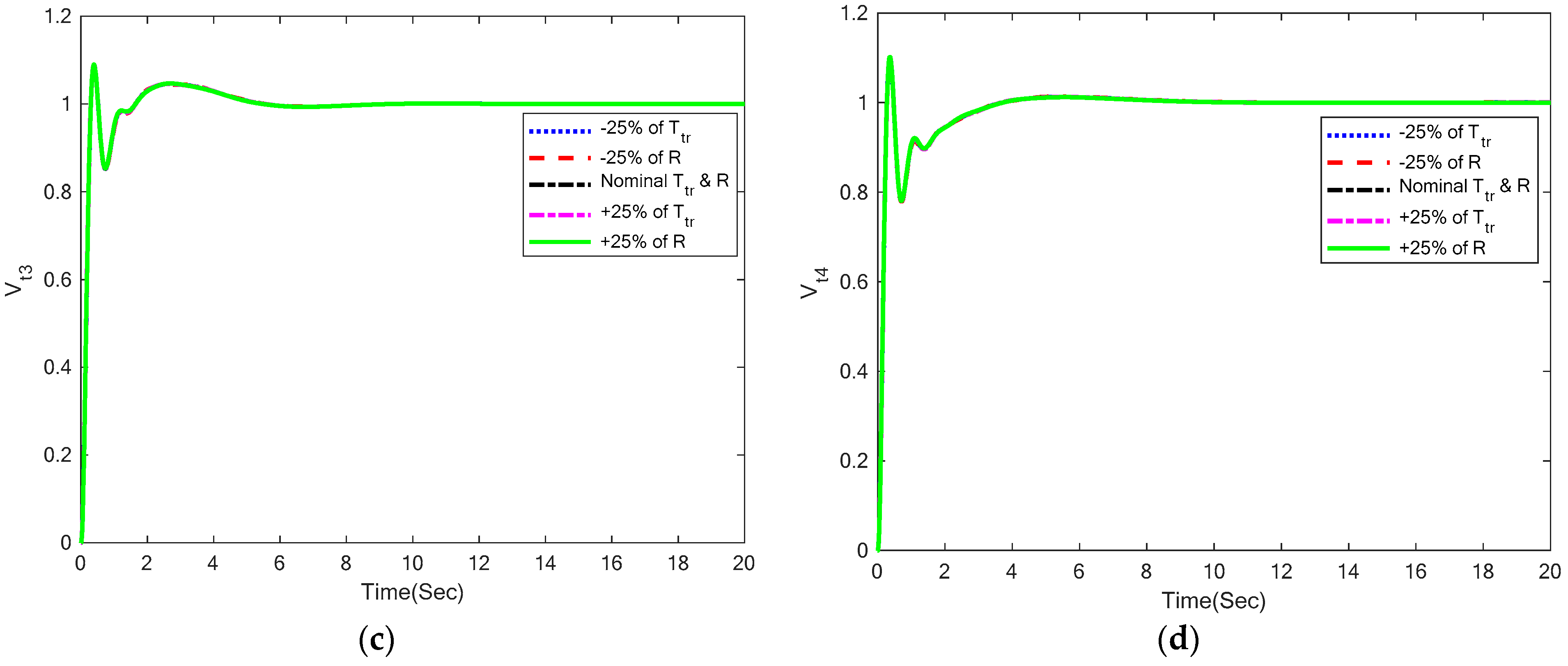
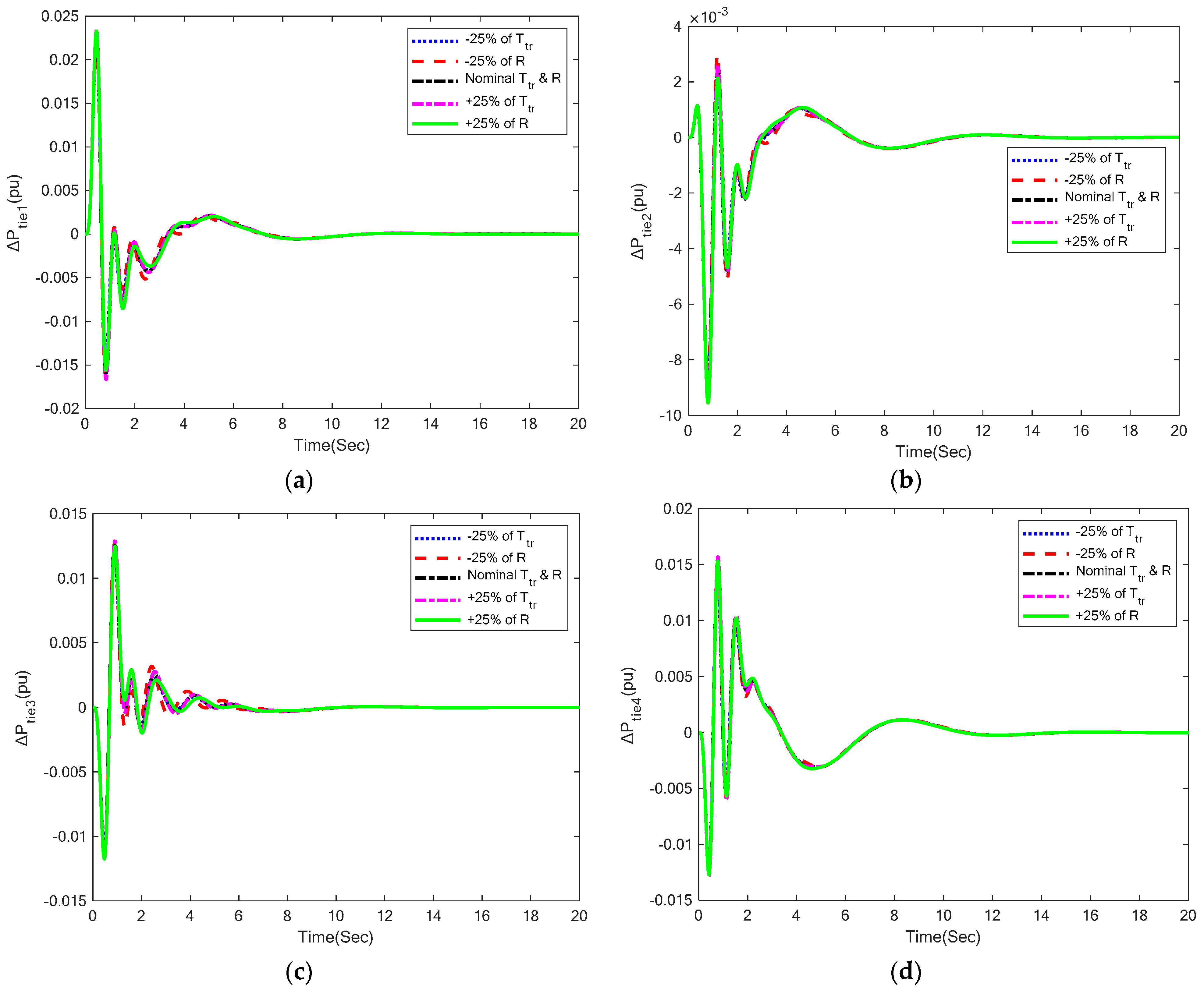
SENSITIVITY ANALYSIS

In this section, the suggested GBO-PID control methodology’s robustness was evaluated using a four-area IPS with a combined LFC-AVR system and dynamic system parameters. The speed regulation (R) and turbine time constant (T_tr) were changed to  ± 25% of their nominal values. In this investigation, the GBO-PID controller’s optimal parameters are taken from Part A. Figure 7, Figure 8 and Figure 9 illustrate the LFC, AVR, and tie-lie power responses of the GBO-PID control methodology with variations in T_tr and R, while

Table 7. Numerical results of LFC with ±25% variations in system parameters using GBO-PID control methodology.

Case	Area-1				Area-2
	Settling Time	% Overshoot	% Undershoot	% s-s Error	Settling Time	% Overshoot	% Undershoot	% s-s Error
−25% of Ttr1, Ttr2, Ttr3, Ttr4	5.23	0.21	−0.57	0	5.26	0.21	−0.53	0
−25% of Rt, Rh, Rg, Rw	6.38	0.26	−0.55	0	6.39	0.24	−0.51	0
Nominal Values	5.37	0.23	−0.58	0	5.38	0.23	−0.54	0
+25% of Ttr1, Ttr2, Ttr3, Ttr4	5.44	0.24	−0.58	0	6.05	0.25	−0.55	0
+25% of Rt, Rh, Rg, Rw	4.89	0.21	−0.60	0	4.90	0.22	−0.56	0
Case	Area-3				Area-4
	Settling Time	% Overshoot	% Undershoot	% s-s Error	Settling Time	% Overshoot	% Undershoot	% s-s Error
−25% of Ttr1, Ttr2, Ttr3, Ttr4	5.27	0.21	−0.51	0	5.28	0.24	−0.49	0
−25% of Rt, Rh, Rg, Rw	6.39	0.21	−0.50	0	6.38	0.25	−0.47	0
Nominal Values	5.38	0.22	−0.52	0	5.98	0.26	−0.49	0
+25% of Ttr1, Ttr2, Ttr3, Ttr4	6.07	0.23	−0.52	0	6.17	0.27	−0.50	0
+25% of Rt, Rh, Rg, Rw	4.90	0.22	−0.53	0	4.92	0.25	−0.51	0

,

Table 8. Numerical results of AVR with ±25% variations in system parameters using GBO-PID control methodology.

Case	Area-1			Area-2
	Settling Time	% Overshoot	% s-s Error	Settling Time	% Overshoot	% s-s Error
−25% of Ttr1, Ttr2, Ttr3, Ttr4	3.95	7.46	0	4.08	5.44	0
−25% of Rt, Rh, Rg, Rw	3.96	7.57	0	4.07	5.43	0
Nominal Values	3.96	7.52	0	4.09	5.45	0
+25% of Ttr1, Ttr2, Ttr3, Ttr4	3.97	7.55	0	4.1	5.46	0
+25% of Rt, Rh, Rg, Rw	3.92	7.40	0	4.07	5.46	0
Case	Area-3			Area-4
	Settling Time	% Overshoot	% s-s Error	Settling Time	% Overshoot	% s-s Error
−25% of Ttr1, Ttr2, Ttr3, Ttr4	4.36	9.0	0	2.91	10.13	0
−25% of Rt, Rh, Rg, Rw	4.36	9.0	0	2.95	10.13	0
Nominal Values	4.36	9.0	0	2.92	10.13	0
+25% of Ttr1, Ttr2, Ttr3, Ttr4	4.36	9.0	0	2.93	10.14	0
+25% of Rt, Rh, Rg, Rw	4.36	9.0	0	2.88	10.14	0

and

Table 9. Numerical results of tie-line power deviation responses with ±25% variations in system parameters using GBO-PID control methodology.

Case	Area-1				Area-2
	Settling Time	% Overshoot	% Undershoot	% s-s Error	Settling Time	% Overshoot	% Undershoot	% s-s Error
−25% of Ttr1, Ttr2, Ttr3, Ttr4	9.39	0.022	−0.015	0	9.71	0.0022	−0.0091	0
−25% of Rt, Rh, Rg, Rw	9.26	0.023	−0.017	0	9.85	0.0029	−0.0089	0
Nominal Values	9.36	0.023	−0.016	0	9.69	0.0025	−0.0093	0
+25% of Ttr1, Ttr2, Ttr3, Ttr4	9.35	0.023	−0.017	0	9.67	0.0026	−0.0094	0
+25% of Rt, Rh, Rg, Rw	9.28	0.023	−0.016	0	9.61	0.0021	−0.0096	0
Case	Area-3				Area-4
	Settling Time	% Overshoot	Undershoot	% s-s Error	Settling Time	% Overshoot	Undershoot	% s-s Error
−25% of Ttr1, Ttr2, Ttr3, Ttr4	8.48	0.012	−0.011	0	10.26	0.014	−0.012	0
−25% of Rt, Rh, Rg, Rw	8.13	0.013	−0.011	0	10.32	0.015	−0.012	0
Nominal Values	8.45	0.013	−0.012	0	10.23	0.015	−0.013	0
+25% of Ttr1, Ttr2, Ttr3, Ttr4	8.47	0.013	−0.012	0	10.21	0.016	−0.013	0
+25% of Rt, Rh, Rg, Rw	7.74	0.012	−0.012	0	10.18	0.015	−0.0013	0

show the numerical results of LFC’s dynamic performance specifications, respectively. Despite the ±25% variance in system parameters, it is clear from the results that all terminal voltage, frequency deviation, and tie-line power deviation responses are nearly identical to one another. The fact that values of all performance specifications including settling time, % overshoot, % undershoot, and steady-state error have barely changed with variation in system parameters is proof that the suggested technique can function well under dynamic circumstances. The results obtained categorically demonstrate that the recommended GBO-PID controller is quite robust and does not require retuning for  ± 25% variations in T_tr and R.

6. Conclusions and Future Work

The transient and steady-state performance of a four-area IPS with combined AVR-LFC was thoroughly examined in this work. The classical PID controller was successfully employed for the efficient control of IPS. The optimal tuning of PID was carried out using a gradient-based optimizer (GBO). Further, the responses of various other controllers such as GBO-I-PD, GBO-TID, and GBO-I-P were compared with the proposed GBO-PID control methodology. With 5% SLP in each area, terminal voltage, frequency deviation, and tie-line power deviation responses of IPS were evaluated. GBO-PID produced a settling time of 5.37 s in area-1, which is 67%, 44%, and 67% in area-1 LFC compared to GBO-I-PD, GBO-TID, and GBO-I-P control methodologies, respectively. GBO-PID delivered a settling time of 5.38 s in area-2, which is 72%, 43%, and 63% in area-2 LFC compared to GBO-I-PD, GBO-TID, and GBO-I-P control methods, respectively. Similarly, GBO-PID generated a settling time of 5.38 s in area-3 which is 51%, 44%, and 70% in area-3 LFC compared to GBO-I-PD, GBO-TID, and GBO-I-P control methodologies, respectively. Moreover, GBO-PID yielded a settling time of 5.98 s in area-4, which is 65%, 38%, and 65% in area-4 LFC compared to GBO-I-PD, GBO-TID, and GBO-I-P control methods, respectively. GBO-PID offered a settling time of 3.96 s area-1 AVR, which is 40% and 47% better than GBO-TID and GBO- I-P control methodologies, respectively. GBO-PID offered settling times of 4.09, 4.36, and 2.92 s in area-2, area-3, and, area-4 AVR, respectively. In comparison to GBO-I-PD, GBO-TID, and GBO-I-P control methodologies, there is 39%, 47%, and 28% better settling time response in area-2 AVR; 24%, 17%, and 38% better settling time response in area-3 AVR; and 45%, 57%, and 51% better settling time response in area-4 AVR, respectively. GBO-PID yielded settling times of 9.36, 9.69, 8.45, and 9.63 s in area-1, area-2, area-3, and area-4, respectively. In comparison to GBO-I-PD, GBO-TID, and GBO-I-P control methodologies, GBO-PID offered considerably better 18%, 72%, and 54% % overshoot response in area-2 AVR. Compared to GBO-I-PD and GBO-TID control methodologies in area-3 AVR, GBO-PID gave comparatively superior 50% and 73% overshoot responses. Further, GBO-PID offered 44%, 16%, and 52% better settling time response in area-1 tie-line power deviation; 50%, 12%, and 40% better settling time response in area-2 tie-line power deviation; 55%, 13%, and 56% better settling time response in area-3 tie-line power deviation compared to GBO-I-PD, GBO-TID, and GBO-I-P control methodologies. Moreover, GBO-PID provided 47% and 44% better tie-line power deviation settling time response as compared to GBO-I-PD and GBO-I-P control methodologies, respectively, in area-4. Hence, it is concluded that GBO-PID performed relatively better as compared to control methodologies. The robustness of GBO-PID was proven by a comprehensive sensitivity analysis with ±25% variations in system parameters. The findings clearly demonstrate the superiority of the suggested GBO-PID control methodology for combined control of load frequency and terminal voltage in multiarea IPS. The proposed methodology can be explored in the future for simultaneous control of terminal voltage and load frequency in a four-area IPS under a deregulated environment and random loading conditions or in the presence of nonlinearities. Further, multiarea IPS with different conventional renewable energy generation units can be examined using GBO-based control methods.

References

1. Ali, T.; Malik, S.A.; Hameed, I.A.; Daraz, A.; Mujlid, H.; Azar, A.T. Load Frequency Control and Automatic Voltage Regulation in a Multi-Area Interconnected Power System Using Nature-Inspired Computation-Based Control Methodology. Sustainability 2022, 14, 12162. [Google Scholar] [CrossRef]
2. Ali, T.; Malik, S.A.; Daraz, A.; Aslam, S.; Alkhalifah, T. Dandelion Optimizer-Based Combined Automatic Voltage Regulation and Load Frequency Control in a Multi-Area, Multi-Source Interconnected Power System with Nonlinearities. Energies 2022, 15, 8499. [Google Scholar] [CrossRef]
3. Vijaya Chandrakala, K.R.M.; Balamurugan, S. Simulated annealing based optimal frequency and terminal voltage control of multi source multi area system. Int. J. Electr. Power Energy Syst. 2016, 78, 823–829. [Google Scholar] [CrossRef]
4. Gupta, M.; Srivastava, S.; Gupta, J.R.P. A Novel Controller for Model with Combined LFC and AVR Loops of Single Area Power System. J. Inst. Eng. Ser. B 2016, 97, 21–29. [Google Scholar] [CrossRef]
5. Sharma, D.; Kushwaha, V.; Pandey, K.; Rani, N. Intelligent AVR Control of a Single Thermal Area Combined with LFC Loop. Adv. Intell. Syst. Comput. 2018, 624, 779–789. [Google Scholar] [CrossRef]
6. Rajbongshi, R.; Saikia, L.C. Coordinated performance of interline power flow controller and superconducting magnetic energy storage in combined ALFC and AVR system under deregulated environment. J. Renew. Sustain. Energy 2018, 10, 044102. [Google Scholar] [CrossRef]
7. Lal, D.K.; Barisal, A.K. Combined load frequency and terminal voltage control of power systems using moth flame optimization algorithm. J. Electr. Syst. Inf. Technol. 2019, 6, 1–24. [Google Scholar] [CrossRef] [Green Version]
8. Sahani, A.K.; Raj, U.; Shankar, R.; Mandal, R.K. Firefly Optimization Based Control Strategies for Combined Load Frequency Control and Automatic Voltage Regulation for Two-Area Interconnected Power System. Int. J. Electr. Eng. Inform. 2019, 11, 747–758. [Google Scholar] [CrossRef]
9. Morsali, J.; Esmaeili, Z. Proposing a New Hybrid Model for LFC and AVR Loops to Improve Effectively Frequency Stability Using Coordinative CPSS. In Proceedings of the 2020 28th Iranian Conference on Electrical Engineering (ICEE), Tabriz, Iran, 4–6 August 2020. [Google Scholar] [CrossRef]
10. Kalyan, C.N.S.; Rao, G.S. Frequency and voltage stabilisation in combined load frequency control and automatic voltage regulation of multiarea system with hybrid generation utilities by AC/DC links. Int. J. Sustain. Energy 2020, 39, 1009–1029. [Google Scholar] [CrossRef]
11. Kalyan, C.N.S.; Rao, G.S. Combined frequency and voltage stabilisation of multi-area multisource system by DE-AEFA optimised PID controller with coordinated performance of IPFC and RFBs. Int. J. Ambient. Energy 2020, 43, 3815–3831. [Google Scholar] [CrossRef]
12. Prakash, A.; Parida, S.K. Combined Frequency and Voltage Stabilization of Thermal-Thermal System with UPFC and RFB. In Proceedings of the 2020 IEEE 9th Power India International Conference (PIICON), Sonepat, India, 28 February–1 March 2020. [Google Scholar] [CrossRef]
13. Nahas, N.; Abouheaf, M.; Darghouth, M.N.; Sharaf, A. A multi-objective AVR-LFC optimization scheme for multi-area power systems. Electr. Power Syst. Res. 2021, 200, 107467. [Google Scholar] [CrossRef]
14. Kalyan, C.N.S. UPFC and SMES based Coordinated Control Strategy for Simultaneous Frequency and Voltage Stability of an Interconnected Power System. In Proceedings of the 2021 1st International Conference on Power Electronics and Energy (ICPEE), Bhubaneswar, India, 2–3 January 2021. [Google Scholar] [CrossRef]
15. Anusha, P.; Patra, S.; Roy, A.; Saha, D. Combined Frequency and Voltage Control of a Deregulated Hydro-Thermal Power System employing FA based Industrial Controller. In Proceedings of the 2021 International Conference on Computational Performance Evaluation (ComPE), Shillong, India, 1–3 December 2021; pp. 848–853. [Google Scholar] [CrossRef]
16. Oladipo, S.; Sun, Y.; Wang, Z. An effective hFPAPFA for a PIDA-based hybrid loop of Load Frequency and terminal voltage regulation system. In Proceedings of the 2021 IEEE PES/IAS PowerAfrica, Nairobi, Kenya, 23–27 August 2021; pp. 1–5. [Google Scholar] [CrossRef]
17. Ramoji, S.K.; Saikia, L.C. Optimal Coordinated Frequency and Voltage Control of CCGT-Thermal Plants with TIDF Controller. IETE J. Res. 2021, 1–18. [Google Scholar] [CrossRef]
18. Safiullah, S.; Rahman, A.; Aftab, M.A.; Hussain, S.M.S. Performance study of ADRC and PID for concurrent Frequency-Voltage Control of Electric Vehicle Incorporated Hybrid Power System. In Proceedings of the 2022 IEEE International Conference on Power Electronics, Smart Grid, and Renewable Energy (PESGRE), Trivandrum, India, 2–5 January 2022. [Google Scholar] [CrossRef]
19. Ramoji, S.K.; Saikia, L.C.; Dekaraja, B.; Behera, M.K.; Bhagat, S.K. Performance Comparison of Various Tilt Controllers in Coalesced Voltage and Frequency Regulation of Multi-Area Multi-Unit Power System. In Proceedings of the 2022 IEEE Delhi Section Conference (DELCON), New Delhi, India, 11–23 February 2022. [Google Scholar] [CrossRef]
20. Dekaraja, B.; Saikia, L.C.; Ramoji, S.K.; Behera, M.K.; Bhagat, S.K. Impact of RFB and HVDC link on Combined ALFC-AVR Studies of a GTPP Integrated Hydro-thermal Systems Using a Cascade Fuzzy PD-TID Controller. In Proceedings of the 2022 4th International Conference on Energy, Power and Environment (ICEPE), Shillong, India, 29 April–1 May 2022. [Google Scholar] [CrossRef]
21. Dekaraja, B.; Saikia, L.C.; Ramoji, S.K. Combined ALFC-AVR Control of Diverse Energy Source Based Interconnected Power System using Cascade Controller. In Proceedings of the 2022 International Conference on Intelligent Controller and Computing for Smart Power (ICICCSP), Hyderabad, India, 21–23 July 2022. [Google Scholar] [CrossRef]
22. Dekaraja, B.; Saikia, L.C.; Ramoji, S.K.; Behera, M.K.; Bhagat, S.K. Performance Analysis of Diverse Energy Storage on Combined ALFC and AVR Control of Multiarea Multiunit System with AC/HVDC interconnection. IFAC-PapersOnLine 2022, 55, 479–485. [Google Scholar] [CrossRef]
23. Fayek, H.H.; Rusu, E. Novel Combined Load Frequency Control and Automatic Voltage Regulation of a 100% Sustainable Energy Interconnected Microgrids. Sustainability 2022, 14, 9428. [Google Scholar] [CrossRef]
24. Kalyan, C.N.S.; Goud, B.S.; Reddy, C.R.; Bajaj, M.; Sharma, N.K.; Alhelou, H.H.; Siano, P.; Kamel, S. Comparative Performance Assessment of Different Energy Storage Devices in Combined LFC and AVR Analysis of Multi-Area Power System. Energies 2022, 15, 629. [Google Scholar] [CrossRef]
25. Daraz, A.; Malik, S.A.; Waseem, A.; Azar, A.T.; Haq, I.U.; Ullah, Z.; Aslam, S. Automatic Generation Control of Multi-Source Interconnected Power System Using FOI-TD Controller. Energies 2021, 14, 5867. [Google Scholar] [CrossRef]
26. Daraz, A.; Malik, S.A.; Mokhlis, H.; Haq, I.U.; Laghari, G.F.; Mansor, N.N. Fitness Dependent Optimizer-Based Automatic Generation Control of Multi-Source Interconnected Power System With Non-Linearities. IEEE Access 2020, 8, 100989–101003. [Google Scholar] [CrossRef]
27. Daraz, A.; Malik, S.A.; Mokhlis, H.; Haq, I.U.; Zafar, F.; Mansor, N.N. Improved-Fitness Dependent Optimizer Based FOI-PD Controller for Automatic Generation Control of Multi-Source Interconnected Power System in Deregulated Environment. IEEE Access 2020, 8, 197757–197775. [Google Scholar] [CrossRef]
28. Daraz, A.; Malik, S.A.; Azar, A.T.; Aslam, S.; Alkhalifah, T.; Alturise, F. Optimized Fractional Order Integral-Tilt Derivative Controller for Frequency Regulation of Interconnected Diverse Renewable Energy Resources. IEEE Access 2022, 10, 43514–43527. [Google Scholar] [CrossRef]
29. Daraz, A.; Malik, S.A.; Haq, I.U.; Khan, K.B.; Laghari, G.F.; Zafar, F. Modified PID controller for automatic generation control of multi-source interconnected power system using fitness dependent optimizer algorithm. PLoS ONE 2020, 15, e0242428. [Google Scholar] [CrossRef]
30. Coban, H.H.; Rehman, A.; Mousa, M. Load Frequency Control of Microgrid System by Battery and Pumped-Hydro Energy Storage. Water 2022, 14, 1818. [Google Scholar] [CrossRef]
31. Tabak, A. Maiden application of fractional order PID plus second order derivative controller in automatic voltage regulator. Int. Trans. Electr. Energy Syst. 2021, 31, e13211. [Google Scholar] [CrossRef]
32. Tabak, A. A novel fractional order PID plus derivative (PIλDµDµ2) controller for AVR system using equilibrium optimizer. COMPEL Int. J. Comput. Math. Electr. Electron. Eng. 2021, 40, 722–743. [Google Scholar] [CrossRef]
33. Krishna, A.K.V.; Tyagi, T. Improved Whale Optimization Algorithm for Numerical Optimization. Adv. Intell. Syst. Comput. 2021, 1086, 59–71. [Google Scholar] [CrossRef]
34. Altbawi, S.M.A.; Bin Mokhtar, A.S.; Jumani, T.A.; Khan, I.; Hamadneh, N.N.; Khan, A. Optimal design of Fractional order PID controller based Automatic voltage regulator system using gradient-based optimization algorithm. J. King Saud Univ. Eng. Sci. 2021. [Google Scholar] [CrossRef]
35. Ayas, M.S.; Sahin, E. FOPID controller with fractional filter for an automatic voltage regulator. Comput. Electr. Eng. 2021, 90, 106895. [Google Scholar] [CrossRef]
36. Rahman, C.M.; Rashid, T.A. A new evolutionary algorithm: Learner performance based behavior algorithm. Egypt. Inform. J. 2021, 22, 213–223. [Google Scholar] [CrossRef]
37. Qais, M.H.; Hasanien, H.M.; Alghuwainem, S. Transient search optimization: A new meta-heuristic optimization algorithm. Appl. Intell. 2020, 50, 3926–3941. [Google Scholar] [CrossRef]
38. Hashim, F.A.; Hussain, K.; Houssein, E.H.; Mabrouk, M.S.; Al-Atabany, W. Archimedes optimization algorithm: A new metaheuristic algorithm for solving optimization problems. Appl. Intell. 2021, 51, 1531–1551. [Google Scholar] [CrossRef]
39. Zhao, S.; Zhang, T.; Ma, S.; Wang, M. Sea-horse optimizer: A novel nature-inspired meta-heuristic for global optimization problems. Appl. Intell. 2022, 1–28. [Google Scholar] [CrossRef]
40. Zhao, S.; Zhang, T.; Ma, S.; Chen, M. Dandelion Optimizer: A nature-inspired metaheuristic algorithm for engineering applications. Eng. Appl. Artif. Intell. 2022, 114, 105075. [Google Scholar] [CrossRef]
41. Wang, L.; Cao, Q.; Zhang, Z.; Mirjalili, S.; Zhao, W. Artificial rabbits optimization: A new bio-inspired meta-heuristic algorithm for solving engineering optimization problems. Eng. Appl. Artif. Intell. 2022, 114, 105082. [Google Scholar] [CrossRef]
42. Zervoudakis, K.; Tsafarakis, S. A mayfly optimization algorithm. Comput. Ind. Eng. 2020, 145, 106559. [Google Scholar] [CrossRef]
43. Ahmadianfar, I.; Bozorg-Haddad, O.; Chu, X. Gradient-based optimizer: A new metaheuristic optimization algorithm. Inf. Sci. 2020, 540, 131–159. [Google Scholar] [CrossRef]
44. Hassan, M.; Kamel, S.; El-Dabah, M.; Rezk, H. A Novel Solution Methodology Based on a Modified Gradient-Based Optimizer for Parameter Estimation of Photovoltaic Models. Electronics 2021, 10, 472. [Google Scholar] [CrossRef]
Figure 1. (a) Combined IPS model (LFC-AVR); (b) tie-line connections.
Energies 16 02086 g001aEnergies 16 02086 g001b
Figure 2. (a) Proposed control methodology. (b) TID controller. (c) I-PD controller. (d) I-P controller.
Energies 16 02086 g002aEnergies 16 02086 g002b
Figure 3. Flow chart of GBO.
Energies 16 02086 g003
Figure 4. LFC responses: (a) ∆f1; (b) ∆f2; (c) ∆f3; (d) ∆f4.
Energies 16 02086 g004
Figure 5. AVR responses: (a) Vt1; (b) Vt2; (c) Vt3; (d) Vt4.
Energies 16 02086 g005
Figure 6. Tie-line power deviation responses: (a) ∆Ptie1; (b) ∆Ptie2; (c) ∆Ptie3; (d) ∆Ptie4.
Energies 16 02086 g006aEnergies 16 02086 g006b
Figure 7. LFC responses with ±25% variations in system parameters (a) ∆f1; (b) ∆f2; (c) ∆f3; (d) ∆f4.
Energies 16 02086 g007
Figure 8. AVR responses with ±25% variations in system parameters: (a) Vt1; (b) Vt2; (c) Vt3; (d) Vt4.
Energies 16 02086 g008aEnergies 16 02086 g008b
Figure 9. Tie-line power deviation responses with ±25% variations in system parameters: (a) ∆Ptie1; (b) ∆Ptie2; (c) ∆Ptie3; (d) ∆Ptie4.
Energies 16 02086 g009