Abstract
With the increasing interdependence among energies (e.g., electricity, natural gas and heat) and the development of a decentralised energy system, a novel retail pricing scheme in the multi-energy market is demanded. Therefore, the problem of designing a customised multi-energy pricing scheme for energy retailers is investigated in this paper. In particular, the proposed pricing scheme is formulated as a bilevel optimisation problem. At the upper level, the energy retailer (leader) aims to maximise its profit. Microgrids (followers) equipped with energy converters, storage, renewable energy sources (RES) and demand response (DR) programs are located at the lower level and minimise their operational costs. Three hybrid algorithms combining metaheuristic algorithms (i.e., particle swarm optimisation (PSO), genetic algorithm (GA) and simulated annealing (SA)) with the mixed-integer linear program (MILP) are developed to solve the proposed bilevel problem. Numerical results verify the feasibility and effectiveness of the proposed model and solution algorithms. We find that GA outperforms other solution algorithms to obtain a higher retailer’s profit through comparison. In addition, the proposed customised pricing scheme could benefit the retailer’s profitability and net profit margin compared to the widely adopted uniform pricing scheme due to the reduction in the overall energy purchasing costs in the wholesale markets. Lastly, the negative correlations between the rated capacity and power of the energy storage and both retailer’s profit and the microgrid’s operational cost are illustrated.
1. Introduction
1.1. Background
Emerging smart grid technologies in the energy system have introduced new opportunities and challenges to both energy suppliers and customers [1]. Local market participants, such as microgrids and local energy communities, have been accelerating the pace of developing distributed energy resources (DERs), which has resulted in the increasing trend in developing integrated local energy systems, including electricity, natural gas and heat energy, and the expanding differences among the microgrids [2]. In this regard, the traditional retail pricing strategy of energy retailers, which offers uniform energy tariffs to customers regardless of their differences, cannot fully unlock the potential benefits of DERs and achieve the potential profit [3]. Therefore, energy retailers would need to consider the interdependence among different energy types from the demand side to make robust and reliable retail pricing decisions. Furthermore, energy retailers also need to take the differences among local customers into consideration to offer customised retail prices to each customer. This calls for a novel customised multi-energy pricing scheme capable of capturing the multi-energy interdependence and characteristics of differentiated customers to be developed for the retail energy markets.
1.2. Literature Review
Retail energy pricing is an important research problem and has been extensively studied in the literature. Ref. [4] systematically investigates and summarises the existence of retail pricing schemes, which demonstrates that the real-time pricing (RTP) strategy can well utilise the demand-side management flexibility over the static pricing strategy, such as the time-of-use (TOU) scheme. Ref. [5] presents a dynamic, real-time energy pricing mechanism to accurately distribute power for the electric vehicles (EVs) charging process fairly when the microgrids are congested. A retail RTP scheme in the presence of hydrogen storage systems and EVs, compared with TOU and fixed pricing schemes, is proposed in Ref. [6]. The bi-objective problem is formulated, in which the average profit needs to be maximised, while the profit deviation should be minimised. The Pareto optimal solution is obtained by the epsilon constraint method and fuzzy satisfying approach. The numerical results show the privilege of the RTP scheme regarding the obtained profit of the retailer. Ref. [7] develops a conditional value at risk (CVaR)-based retail electricity pricing scheme to reduce the impact of risk caused by the uncertainties from RES generation and estimated wholesale electricity prices. An energy management and pricing method for the community energy retailer incorporating smart building consumers is investigated in Ref. [8]. The numerical results, which are solved by the bilevel chance-constrained programming approach, show that the proposed approach can benefit both retailers and customers. Lastly, Ref. [9] proposes a bilevel game-theoretic model for multiple strategic retailers’ decision-making problems, which include the retail prices in the retail market, bid prices in the day-ahead wholesale market, and the bid/offer prices in the local power exchange market. The problem is formulated as an equilibrium problem with the equilibrium constraints (EPEC) problem, which is solved by the diagonalisation algorithm.
The majority of the existing literature focuses on developing a retail pricing strategy in the electricity market, whereas only few studies analyse the retail pricing problem in a multi-energy context. In addition, since the development of a multi-energy pricing scheme consists of energy suppliers (e.g., retailers) and customers (e.g., microgrids and aggregators), a bilevel optimisation model, which can well present the intrinsic hierarchical structure of the energy system, has been widely adopted in the literature. For instance, Ref. [10] proposes a bilevel optimal retail pricing scheme for the retailer and multi-energy buildings to perform the price-based DR programs. A bilevel stochastic RTP model in the framework of the Markov decision process is formulated for the multi-energy system in Ref. [11]. A novel distributed online multi-agent reinforcement learning algorithm is developed to solve the proposed model. Ref. [12] proposes a bilevel multi-energy trading model between the multi-energy service provider and consumer by setting the optimal energy pricing scheme and energy economic dispatch at the upper level. Optimal consuming patterns of different energies are obtained for the multi-energy consumer in the lower-level problem. Ref. [13] develops an integrated energy service provider (IESP) as a retailer to effectively set energy prices and energy management in the multi-energy market. The impact of DR and wholesale prices’ uncertainties is considered in the proposed two-stage stochastic hierarchical framework. The day-ahead energy pricing and management method considering multi-energy DR programs for IESP in regional integrated energy systems is addressed in Ref. [14]. The bilevel Stackelberg game optimisation model is established and shows that the pricing scheme benefits both the energy supplier (i.e., IESP) and consumer. The pricing behaviour of multi-energy players who can trade electricity, natural gas and heat energy to maximise their profits and reduce their operational risk is studied in Ref. [15]. The bilevel approach is applied to model the decision-making conflict of the multi-energy players with other energy players participating in the multi-energy system.
The bilevel optimisation model is typically solved by analytical mathematical methods, such as the Karush–Kuhn–Tucker (KKT)-based reformulations in the literature [10,12,13,14,15]. However, the premise of applying those methods may include the convexity of the lower-level problem. For the bilevel model, whose lower-level problem is proved as non-convex, such as including integer variables, traditional mathematical approaches cannot solve it effectively. Therefore, many metaheuristic algorithms, such as PSO, GA and SA, are introduced in the literature to overcome the non-convexity of the lower-level problem [16]. For instance, Ref. [17] develops a hierarchical market framework to apply real-time retail pricing between an energy supplier and multi-energy microgrids, where a hybrid solution method combining PSO and the branch and bound algorithm is proposed. In Ref. [18], a dynamic pricing profile is developed for utilising distributed energy storage and overcoming the intermittency from renewable generation. A novel non-cooperative Stackelberg game is proposed to formulate the pricing problem, in which the upper-level problem is solved by the PSO algorithm, and linear programming is applied at the lower level. In addition, Ref. [19] presents a bilevel price decision model for a load-serving entity to manage multiple multi-energy microgrids with DR. The microgrids’ operation problems are formulated at the lower level and solved by a MILP program. A GA algorithm is applied to find the optimal price decisions for the load-serving entity at the upper level. A real-time pricing strategy is proposed in Ref. [20] to effectively adjust the power balance between the supply and demand and manage the microgrid’s internal energy dispatch. The pricing strategy is formulated as a bilevel programming model, where the supplier’s price decision making at the upper level is solved by the GA algorithm. Ref. [21] develops a SA-based price control algorithm to solve the non-convex real-time pricing problem, which can reduce the peak-to-average load ratio and retailer’s cost through DR management in smart grid systems. Ref. [22] proposes a bilevel Stackelberg game to model hierarchical interactions between one profit-seeking energy retailer and multiple cost-minimising energy customers. A GA algorithm is developed to solve the bilevel model. Lastly, Ref. [23] proposes a bilevel model, where data-driven appliance-level customer behaviour learning models are developed at the lower level. The resulting hybrid optimisation–machine learning bilevel model is solved by GA.
The retail pricing schemes mentioned in the above literature are classified into the uniform pricing scheme, where the decision maker optimises the pricing decisions without considering the different characteristics among underlying energy customers, such as the demand-side load profile and the specifications of the equipped DERs, such as energy converters and storage. Therefore, the elasticity on the demand-side management of each energy customer cannot be fully utilised under the uniform pricing scheme. To conquer the deficiency of the widely used uniform pricing scheme, a novel customised energy pricing scheme should be developed that takes the unique characteristics of each customer into consideration. It is designed to motivate the potential flexibility of demand-side management to benefit market participants, such as energy retailers. However, only few studies address the customised retail energy pricing problem in the literature. For instance, Ref. [24] develops a bilevel model for optimal differential pricing considering different customer groups characterised by different price sensitivities. Ref. [25] proposes a customised TOU electricity pricing scheme for different residential users depending on their load-consumption profiles, which is established based on the bilevel optimisation framework. The problem of customising TOU electricity retail prices based on load profile analysis by applying a clustering algorithm is addressed in Ref. [26]. Similarly, a realistic multiple dynamic pricing scheme for the segmented customers based on the different identification of load patterns is proposed in Ref. [3], which demonstrates the effectiveness of the clustering-based approach. Furthermore, the electricity retailer could achieve better profit gain under the proposed multiple pricing scheme. Ref. [27] presents a personalised RTP scheme using a bilevel model to improve the management of different electricity consumption, including both traditional and renewable energies. Ref. [28] proposes a bilateral energy-trading structure to coordinate the hierarchical personalised electricity pricing model between the energy trading agent and energy prosumers.
The above reviewed literature is compared and summarised in Table 1. Although the above studies provide valuable insights regarding the customised retail pricing scheme, they are limited to electricity markets. Therefore, to the best of our knowledge, there is no existing research studying the customised multi-energy pricing problem. To fill the research gap following the above analysis, in this paper, we propose a novel customised multi-energy pricing scheme for an energy retailer that manages multiple microgrids in the multi-energy market.

Table 1.
Literature comparison. ✓: Yes; ✗: No; –: Not applicable.
1.3. Contributions
The main contributions of this paper are summarised as follows:
- A bilevel optimisation model is developed to formulate the novel customised pricing scheme for an energy retailer that manages multiple microgrids in the multi-energy market. In particular, a retailer’s profit maximisation problem is considered at the upper level. The energy management for each microgrid is detailed, and the operational cost minimisation is formulated at the lower level.
- The detailed energy management model for each microgrid equipped with energy converters (i.e., combined heat and power (CHP) and heat pump), electrical and thermal storage, RES (i.e., solar and wind) and DR programs (i.e., load curtailment and shifting) is formulated as a MILP program at the lower level. Specifically, load curtailment refers to the reduction in energy consumption, while in the load-shifting program, the electricity demand can be rescheduled and shifted to other scheduling hours.
- Three hybrid metaheuristic algorithms (i.e., PSO, GA and SA) combined with the conventional MILP program are developed to solve the proposed bilevel problem. The hybrid solution algorithms conquer the non-convexity of the lower level problems, which are proved difficult to solve with traditional mathematical methods, such as KKT-based solution methods. In numerical analyses, we test the performance of the three algorithms. The comparison between the customised and uniform pricing schemes is illustrated in detail. In addition, the effect of the rated capacity and power of electrical and thermal storage on the energy retailer’s pricing decisions, profit, and microgrids’ operational costs is thoroughly investigated.
1.4. Paper Organisation
The remainder of this paper is organised as follows. In Section 2, the proposed bilevel model is discussed in detail. Section 3 describes the three hybrid metaheuristic algorithms combined with the MILP program. The numerical results are presented in Section 4. Finally, the conclusion is drawn in Section 5.
2. Model Formulation
This section shows the formulation of the proposed bilevel optimisation model. In particular, Section 2.1 presents an overview of the bilevel MILP model. The customised multi-energy pricing problem is described in Section 2.2. Lastly, the lower and upper level model formulations are discussed in Section 2.3 and Section 2.4, respectively.
2.1. Bilevel MILP Model Overview
Bilevel optimisation refers to one of the categories of optimisation that copes with the problem with a hierarchical structure in nature, which includes two decision makers (i.e., leader and follower) located at the upper and lower levels, respectively. The bilevel model is formulated by an optimisation problem (lower level) embedded into another problem (upper level). The problem originates from the game theory in economics and was introduced by Heinrich Freiherr von Stackelberg in 1934 [29]. The decision variables of a bilevel model can be continuous and discrete. Since formulating the customised multi-energy pricing problem involves integer variables in the lower-level problem, in this section, an overview of the bilevel MILP model is introduced as follows.
The general form of a bilevel MILP model with a single leader and multiple independent followers is shown below:
Subject to:
where and are the feasible solution sets for both upper and lower level problems. The set of followers is denoted as . n and indicate the number of decision variables for the leader and the follower . and represent the objective functions for the upper and lower level problems. On the other hand, the upper and lower level constraint functions are indicated as and , respectively. Notice that is the set of indices that the corresponding are integer variables.
If denotes the vector of the leader’s decision variables, the feasible solution and rational reaction sets of each follower i can be represented as and . Finally, the bilevel MILP feasible set, which is also called the inducible region, is presented as . The optimal solution of the bilevel model is denoted as .
2.2. Customised Multi-Energy Pricing Problem Description
In the proposed multi-energy market, which is shown in Figure 1, multiple microgrids are managed by a single energy retailer that purchases electricity and natural gas from the upstream wholesale markets. The microgrids are allocated with CHP, heat pump, electrical and thermal storage, RES and DR programs, which operate their energy management systems. Therefore, given the ability of microgrids to generate and transfer energy, the energy retailer can also purchase the electricity from the managed microgrids and sell it back to the wholesale market to make a profit. In addition, the detailed framework of the proposed bilevel model is presented in Figure 2. Particularly, at the upper level, to maximise the profit, the energy retailer optimises the retail pricing decisions based on the proposed customised multi-energy pricing scheme within the scheduling hours and announces them a day ahead to each microgrid i, respectively. After receiving the corresponding retail energy prices, each microgrid i reacts by minimising its operational cost and reports the volume of energy to be exchanged (buy or sell) to the retailer. As a result, each microgrid’s optimal customised retail pricing scheme and energy management are obtained. The detailed model formulations for both the lower and upper levels are shown in Section 2.3 and Section 2.4 below.
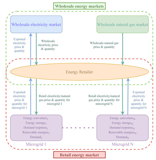
Figure 1.
Structure of the multi-energy market.
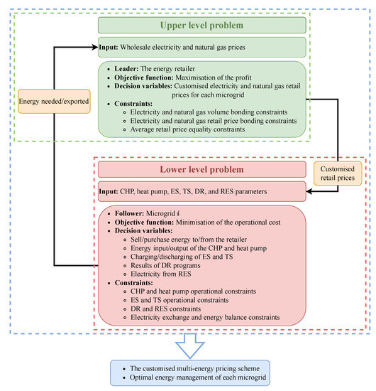
Figure 2.
Framework diagram of the proposed bilevel model.
2.3. Follower-Side/Lower-Level Problem
It is assumed that the microgrids in managed by the energy retailer operate independently at the lower level. In this section, the detailed lower-level formulations for the microgrid are shown as follows.
2.3.1. Lower-Level Objective Function
The lower-level objective function (1) shows the total operational costs of the microgrid i. In particular, the first group of elements presents the energy exchange between the microgrid i and the retailer. and denote the amount of electricity and natural gas that the microgrid i purchases from the retailer. represents the amount of electricity that the microgrid i exports to the retailer. and denote the retail electricity and natural gas prices that the energy retailer announces to the microgrid i. Notice that the price of electricity sold by the microgrid i back to the retailer is proportional to the retail electricity price, denoted as . The second and third groups of elements describe the CHP and heat pump costs, respectively, including operation and maintenance costs ,, start-up cost , and shut-down cost ,. The fourth group of elements represents the electrical and thermal storage costs, which are denoted as and . The last group of elements shows the costs of the load curtailment program for all energies, which are denoted as , , and .
2.3.2. CHP Operational Constraints
The CHP unit, which converts natural gas into electricity and heat, is formulated in (2a)–(2m) inspired by Ref. [30]. The energy conversion constraints of the CHP are denoted in (2a) and (2b). represents the amount of natural gas consumed by the CHP. and denote the amount of electricity and heat generated by the CHP. The energy conversion efficiencies for different energies are denoted as and , respectively. The limitation of the CHP electricity output is shown in (2c), where denotes the CHP operational status. (2d)–(2g) represent the ramp-up and ramp-down power constraints of the CHP electricity output. The initial status of the CHP is denoted as . represents the last amount of CHP generated electricity during the last scheduling hours. and show the maximum amount of ramp-up and ramp-down electricity. In addition, the start-up and shut-down actions of the CHP are described in (2h)–(2l), where and denote the CHP start-up and shut-down statuses. Lastly, (2m) presents the binary variables that appear in the CHP operation:
2.3.3. Heat Pump Operational Constraints
The heat pump generates heat energy by consuming electricity. Equation (3a) is the energy conversion constraint. and denote the amount of electricity consumed and the amount of heat generated by operating the heat pump. denotes the energy conversion efficiency. The amount of generated heat is bounded in (3b), where the heat pump operational status is presented as . The ramp-up and ramp-down constraints of the heat pump are depicted in (3c)–(3f), where denotes the final amount of heat generated by the heat pump in the last scheduling hours. The maximum amount of ramp-up and ramp-down heat are represented as and , respectively. (3g)–(3k) define the heat pump start-up and shut-down actions, whose corresponding start-up and down statuses are denoted as and . The binary variables in this operation are shown in (3l):
2.3.4. Electrical Storage (ES) Operational Constraints
Constraints (4a) and (4b) describe the change of the ES energy level considering charging rate , discharging rate , and self-discharging rate . and denote the amount of charged and discharged electricity. (4c) limits the energy level of the ES in each scheduling hour. In addition, for operational purposes, (4d) ensures that the energy level of the ES stays unchanged after the scheduling hours. and denote the final and initial energy level of the ES. The charging and discharging power are bounded in (4e)–(4h), where and represent the charging and discharging statuses:
2.3.5. Thermal Storage (TS) Operational Constraints
The operational constraints of TS are similar to ES. Specifically, the TS energy level is represented in (5a) and (5b), where , , and denote the TS energy level, charging rate, discharging rate and self-discharging rate, respectively. and present the amount of charged and discharged heat. The TS energy level in each scheduling hour is bounded in (5c). The initial and final energy levels , of the TS are imposed to be equal in (5d). Constraints (5e)–(5h) constrain the charging and discharging power of the TS, where and represent the TS charging and discharging statuses:
2.3.6. DR Programs Constraints
Two types of DR programs are considered in microgrid i, which are load curtailment (LC) and load shifting (LS), which are formulated in (6a)–(6c) and (6d)–(6h), respectively. Both formulations of the DR programs are inspired by Ref. [30]. The detailed description and formulation are shown below.
Load curtailment:
It is assumed that the electricity, natural gas, and heat demand can all be curtailed during the scheduling hours, and the curtailment rates are denoted as , , , respectively. The bounding constraints for the three types of energies are presented in (6a)–(6c). Notice that the curtailable energy demand in each scheduling hour is predetermined by the energy retailer and represented as , and :
Load shifting:
We assume there are households in that participate in the load-shifting program. Each household has the load-adjustable time window , which is represented in (6d). denotes the household’s operational status. The start and stop times of the load-shifting program for each household are denoted as and . Constraint (6e) imposes that there is no shiftable load available in the scheduling hours outside of the adjustable time window. The shiftable load in each scheduling hour is flexible but bounded in (6f). Finally, (6g) makes sure the overall electricity consumption is not affected by the load-shifting program:
2.3.7. RES Constraints
Two renewable energies, solar and wind power, which are generated by photovoltaics (PV) and wind turbines (WT) are considered in this paper. To reduce the effect of the uncertainties of the renewable energies in nature, the bounding constraints of the forecast of PV and wind powers in each scheduling hour are introduced in (7a) and (7b):
In addition, inspired by Ref. [31], the spinning reserve constraint (7c) is implemented to further maintain and secure the operation of microgrids and the power system. It presents that the maximum power supply of the microgrid i must be sufficient to provide at least times load demand in each scheduling hour. denotes the spinning reserve ratio:
2.3.8. Microgrid Electricity Exchange Constraints
The electricity imported to and exported from the microgrid i are constrained in (8a) and (8b), where the importing and exporting statuses are denoted as and , respectively. Additionally, (8c) imposes that electricity import and export cannot happen simultaneously:
2.3.9. Energy Balance Constraints
The demand and supply balance constraint for each type of energy in the multi-energy system must be satisfied at every scheduling hour. Constraints (9a)–(9c) represent the energy balance constraints of electricity, natural gas, and heat, respectively. , , and denote the critical/base demand for each type of energy:
The decision variables of the lower-level problem for the microgrid i are . Notice that the lower-level problem of each microgrid forms a MILP problem, which can be solved efficiently by off-the-shelf commercial solvers, such as CPLEX and GUROBI.
2.4. Leader-Side/Upper-Level Problem
We assume that the energy retailer manages multiple multi-energy microgrids by adopting the proposed customised multi-energy pricing scheme. The profit maximisation problem of the retailer is formulated at the upper level and shown as follows:
subject to
The decision variables of the upper-level problem are , which denote the retail electricity and natural gas prices for each microgrid at each scheduling hour. The objective function (10a) depicts the overall profit of the retailer. and denote the wholesale electricity and natural gas prices. In particular, the first group of elements in (10a) represents the revenue obtained from all microgrids by exchanging electricity. The electricity purchasing cost from, or the selling revenue to, the wholesale electricity market is described in the second group of elements. The last group of elements denotes the profit of selling natural gas to the microgrids. Constraints (10b) and (10c) limit the amount of electricity and natural gas exchange between the energy retailer and wholesale markets. The retail electricity and natural gas prices customised for each microgrid are bounded in (10d) and (10e). Constraints (10f) and (10g), which are inspired by Ref. [3], impose the average retail electricity and natural gas prices within the scheduling hours to be equal to the predetermined constants and . Notice that the two equality constraints ensure a sufficient number of low price scheduling hours. Without these constraints, in principle, the retailer could always choose the maximum retail prices to maximise its profit. As a result, the constraints provide a fair retail price image among microgrids, which are also crucial for the retailer’s market share in the long term [32].
3. Solution Methods
The proposed bilevel model includes many binary decision variables in the lower-level problems, which make it extremely hard to solve by conventional analytical methods, such as KKT reformulation-related methods. To overcome the non-convexity of the model, we propose three categories of metaheuristic algorithms that simulate the behaviours of the energy retailer at the upper level to find an optimal solution efficiently, which are as follows: swarm-based, PSO; evolution-based, GA; and physics-based, SA. Therefore, the three metaheuristic algorithms combined with the lower-level MILP solver form different hybrid solution algorithms, which are illustrated in detail below.
3.1. PSO-Based Algorithm
The PSO algorithm is a swarm-based metaheuristic method that simulates the social behaviour of the movement of organisms in a bird flock or fish school [33]. Namely, when birds search randomly for food, for instance, all birds in the flock are able to share their knowledge and discovery to help the entire flock find the best location for hunting. Figure 3 shows the flowchart of the proposed PSO-based algorithm. Essentially, each particle contains two properties: position and velocity. During each iteration, the global best position of all particles and the best previously visited position of each particle are found by evaluating the fitness function of each particle. Each particle’s position and velocity are updated via the equations as follows:
where the superscript y indicates the number of iterations, w denotes the inertia weight, and represent cognitive constant and social constant, respectively, and and are uniformly distributed random numbers in . Notice that if any element in the updated particle position is out of the boundary set by (10d) and (10e), the nearest boundary is assigned to the element [34].
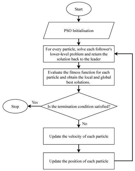
Figure 3.
Flowchart of the PSO-based algorithm.
The detailed process of the PSO-based decision-making algorithm is shown in Algorithm 1. In particular, the maximum iteration, total number of particles and each particle’s position x and velocity v need to be initialised. Notice that each particle’s position denotes the energy retailer’s customised pricing decision for the next 24 h. Steps 3–7 show the interaction between the energy retailer and microgrids and are interpreted as follows. First, the energy retailer announces the customised electricity and natural gas prices for each microgrid for the next 24 h in step 4. Then, each microgrid solves its energy-management problem based on the received energy prices from the retailer and obtains the optimal solution, which is returned back to the energy retailer in step 5. In step 6, after receiving the optimal energy management solutions from all microgrids, the energy retailer solves its profit maximisation problem and evaluates the current pricing decisions using the fitness function based on the penalisation method proposed by [35,36]. Notice that the penalised fitness function formulation can not only be used for the PSO-based algorithm but also be applied to GA- and SA-based algorithms since the constraint-handling technique can be generalised in metaheuristic algorithms. When the predefined termination condition is not satisfied, the global best position of all particles and the personal best previously visited position of each particle are recorded in steps 11 and 12. Each particle’s position and velocity are then updated by applying (11a) and (11b) in step 13. The algorithm iterates until the termination condition is reached and outputs the optimal solutions for the energy retailer and each microgrid.
| Algorithm 1 PSO-based algorithm. |
|
3.2. GA-Based Algorithm
GA algorithm is an evolution-based computational method inspired by genetics and natural selection [37]. The flowchart of the GA-based algorithm is shown in Figure 4. In particular, after evaluating the population of the current generation, the elite chromosome with the best fitness value is inherited by the next generation. Furthermore, the selection process, such as the roulette wheel, tournament and random selection, is applied to choose other chromosomes for the next generation. The chromosomes of the successive generation are finally generated by crossover and mutation processes [22]. Algorithm 2 explains the process of the solution algorithm. Firstly, the maximum iteration and population of chromosomes are initialised. Similar to the PSO-based algorithm, each chromosome indicates the energy retailer’s pricing decisions, and steps 3–7 show the retailer and microgrids’ interactions. Then, the next generation of chromosomes is created by applying selection, crossover and mutation in step 11. Specifically, the stochastic uniform selection method is used to choose the next generation of chromosomes. The scattered crossover function is applied by creating a random binary vector and selecting the genes from the first parent chromosome when the entry is 1 and from the second parent chromosome when the entry is 0. Lastly, the Gaussian mutation is utilised to explore the search space, which adds a random number taken from the Gaussian distribution with a mean 0 to each gene of the chromosome. The algorithm is stopped when repeating steps 3–12 until the termination condition is satisfied.
| Algorithm 2 GA-based algorithm. |
|
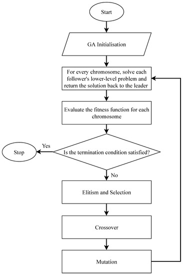
Figure 4.
Flowchart of the GA-based algorithm.
3.3. SA-Based Algorithm
Simulated annealing is a physics-based probabilistic approach that emulates the standard annealing process used in metallurgy to improve the properties of solids. Essentially, after the solid is heated up by a significantly high temperature, the atoms gain the energy to explore their stable states. The optimal state of each atom can be then found following the annealing process. As a result, the solid is recrystallised and improves its ductility. Similarly, the simulated annealing algorithm is applied to find the optimal solution by cooling the heated atoms in the search space. Figure 5 shows the flowchart of the SA-based algorithm. In particular, it uses the Metropolis algorithm to generate the next trial atoms by randomly perturbing the current ones. If the fitness value of the trial atom is greater than the current fitness value, the trial atom replaces the current atom in the next iteration. Otherwise, the trial atom can still be accepted by the acceptance criterion, which is based on the Boltzmann distribution shown in (12a) [38]:
where represents the difference of fitness values between the trial atom and current atom . The temperature in the current iteration is denoted as . Notice that when the temperature is significantly high, the SA algorithm can accept the worse solution, which is particularly beneficial in search space exploration. As the temperature drops in every iteration, the acceptance criterion also decreases, which leads to the lower possibility of accepting the worse solution. The SA algorithm can be considered to be the hill climbing algorithm when the temperature is significantly low (e.g., 1), which takes advantage of the efficient local search method.
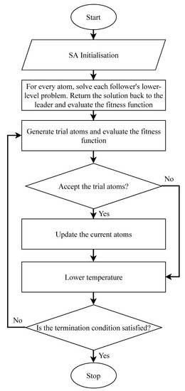
Figure 5.
Flowchart of the SA-based algorithm.
Algorithm 3 shows the proposed SA-based algorithm to solve the bilevel model. The maximum iteration, total number of atoms, and initial and final temperature are initialised in step 1. Steps 2–7 are similar to Algorithms 1 and 2, which present the interactions between the retailer and microgrids. In step 8, the energy retailer proposes a trial energy prices decision for each current price strategy and collects the evaluation by repeating steps 5 and 6. If the fitness value from the trial prices is higher than the current ones, the retailer replaces the current prices with the trial prices in the next iteration. Otherwise, the retailer decides the accept or refuse the trial prices based on the acceptance criterion (12a). This decision process is illustrated in steps 9–12. The temperature decreases in every iteration in step 13. The algorithm repeats steps 8–16 until the termination condition is fulfilled.
| Algorithm 3 SA-based algorithm. |
|
4. Numerical Results
The section discusses the results of numerical analyses to illustrate the feasibility and effectiveness of the proposed bilevel model and the solution algorithms. In particular, Section 4.1 describes the setup for the experiments. The three aforementioned metaheuristic algorithms for solving the proposed bilevel model are compared and analysed in Section 4.2. Moreover, the performance results of the proposed customised and the uniform multi-energy pricing schemes are investigated in Section 4.3. Lastly, Section 4.4 presents the effect of the rated capacity and power of the ES and TS on the retailer’s profit and the microgrids’ operations.
4.1. Experimental Setup
In this section, we consider three different microgrids (i.e., microgrid 1, microgrid 2 and microgrid 3) that are managed by the energy retailer. Each microgrid’s base demand and the configurations of its facilities (i.e., the capacity and rated power of ES and TS) are differentiated from others. The base electricity, natural gas, and heat demand for each microgrid come from the PJM dataset [39], United Kingdom Department of Education Gas dataset [40], and Open Power System Data [41], respectively, which are shown in Table A1. Each microgrid’s ES and TS parameter setups are shown in Table 2 and Table 3. Besides the ES and TS parameter setup, other facilities, such as CHP, heat pump, and load-shifting programs, share the same parameters among microgrids, shown in Table A2, Table A3 and Table A5. The minimum power of RES is zero, while the maximum power for each scheduling hour is shown in Table A4, which originated from [42,43]. The wholesale electricity and natural gas prices come from [44], which are presented in Table A6. In addition, the curtailable load and costs of electricity, natural gas and heat are 300 MWh, 100 kcf and 350 MBtu, and $70/MWh, $20/kcf and $60/MBtu, respectively. The minimum and maximum curtailment rates are 0 and 0.4. For each microgrid, the minimum and maximum electricity purchased from and exported to the energy retailer are 0 MWh and 5000 MWh, respectively. For the energy retailer, the minimum and maximum retail electricity prices are $60/MWh and $110/MWh, and $15/kcf and $60/kcf for the natural gas prices. The electricity price that each microgrid sells back to the energy retailer is set to be 90% of the current retail price. The average retail electricity and natural gas prices are predetermined as $90/MWh and $40/kcf.
Table 2.
ES parameters. – : Not applicable.
Table 3.
TS parameters. – : Not applicable.
All three hybrid algorithms are written in MATLAB R2022b and run on Windows 11 Pro 64-bit with 12 cores CPU @ 3.6 GHz and 32 GB of RAM. The coupled MILP problem is solved by Gurobi Optimiser (version 10.0.0) using the branch and bound algorithm. Each iteration for all three hybrid algorithms consists of upper-level operations and 600 (200 individuals × 3 microgrids) lower-level MILP problems, which takes about 60 s to complete.
For the hybrid solution algorithms, we consider 100 iterations for a single run, which includes a population of 200 individuals (price signals). In particular, for the PSO-based algorithm, the inertia weight is 1.1. The cognitive and social constants are both 1.49. For the GA-based algorithm, the best 10 elite chromosomes are survived to the next generation. In the SA-based algorithm, the initial and final temperatures are 100 and 1 degrees. Notice that all parameters are set after a mass of experiments, considering the balance between the quality of results and computation burden.
4.2. Solution Algorithms Comparison
The principal focus of this section is the numerical comparison among the aforementioned hybrid solution methods, i.e., PSO, GA and SA coupled with MILP algorithms. In this experiment, the three hybrid algorithms run 25 times independently for both proposed customised and uniform pricing models. The detailed statistical analysis of the results of the energy retailer’s profit is shown in Table 4. For the customised pricing scheme, the GA-based algorithm presents outstanding performance along with others, obtaining higher minimum, maximum, median and average values of the retailer’s profit. Furthermore, the standard deviation and interquartile range (IQR) that measures the spread of the middle 50% of the data are the lowest using the GA-based algorithm, which indicate less data dispersion. On the other hand, for the uniform pricing scheme, although the standard deviation of SA-based results is the lowest among others, the GA algorithm still reveals significantly high values in all minimum, maximum, median and average statistical measurements. In summary, the GA-based algorithm is verified to provide the best performance for both customised and uniform pricing models, considering the value and stability of the results it can achieve. Therefore, the GA-based hybrid algorithm is applied to solve customised and uniform pricing models in the following experiments.
Table 4.
Statistical results of three hybrid solution algorithms.
4.3. Customised and Uniform Multi-Energy Pricing Schemes
This section presents the difference between the performance of customised and uniform pricing schemes. Notice that the results come from the GA-based algorithm, which runs 25 times independently in the previous section. The cost and revenue of the retailer, net profit margin and each microgrid’s cost are calculated based on the run, which generates the median value of the retailer’s profit. The two pricing schemes are compared in Table 5. It reveals that the energy retailer can make more profit under the customised pricing scheme measured by both the average (+0.90%) and median (+2.08%) profit value. This is because the customised retail prices are tailored to each microgrid with different characteristics and load patterns, which makes the retailer’s pricing decisions more flexible. In addition, Table 6 shows the microgrids’ energy management results under the two pricing schemes. Specifically, except for the operational cost, all other values in Table 6 are the sum of the particular result over the 24 scheduling hours. Notice that the amount of the microgrids’ purchased energy is identical to the amount of energy the retailer bids from the wholesale markets. It turns out that the retailer purchases 7.93% less electricity and buys 3.84% more natural gas under the customised pricing scheme because natural gas is cheaper than electricity. Since the retailer costs less to purchase energy from the wholesale markets and gains the ability to customise the pricing strategy for each microgrid, the retailer’s profit is increased compared to that under the uniform pricing scheme. Moreover, because the customised pricing scheme obtains higher profit with relatively less revenue, the retailer’s net profit margin, which measures the amount of profit the retailer obtains per dollar of revenue gained, is 1.01% larger compared to the uniform pricing scheme. As a result, the proposed customised pricing scheme is superior to the uniform pricing scheme and beneficial for the retailer to acquire more profit and a higher net profit margin.
Table 5.
Results of retailer under customised and uniform pricing schemes.
Table 6.
Microgrids energy management results under customised and uniform pricing schemes. – : Not applicable.
Each microgrid’s energy demand under the customised pricing scheme is less than or equal to the demand under the uniform pricing scheme. This can show the effectiveness of the load curtailment program. Moreover, the CHP is heavily used as a cheaper alternative to generate electricity under the customised pricing scheme. On the contrary, the heat pump is less implemented since more heat demand is satisfied by the CHP. Additionally, because the rated capacity and power of the ES and TS in microgrid 3 are significantly larger than those in microgrid 2, the microgrid’s ES and TS charging and discharging power is remarkably greater than those of microgrid 2 under both pricing schemes.
4.4. Effect of ES and TS Rated Capacity and Power
One of the objectives in this section is to identify the effect of rated capacity and power of the ES and TS on the profit of the energy retailer. We consider three different scenarios to illustrate these effects. The identical base energy load demand (i.e., the base energy demand in microgrid 1) is applied for all three microgrids. In the first scenario (Scenario 1), each microgrid has differentiated ES and TS configurations (shown in Table 2 and Table 3). Notice that microgrid 1 does not equip either ES or TS. The rated capacity and power of ES and TS for microgrid 2 are 500 MWh and 200 MW/h, 600 MBtu and 200 MBtu/h. For microgrid 3, the rated capacity and power of ES and TS are 1000 MWh and 300 MW/h, and 1300 MBtu and 430 MBtu/h. In the second scenario (Scenario 2), none of the three microgrids are equipped with ES and TS. On the other hand, all three microgrids in the third scenario (Scenario 3) own the same configurations of ES and TS, which are the same as those of microgrid 3 in Scenario 1. Additionally, we analyse the retailer’s profit and microgrids’ operational costs over 15 independent runs for each scenario to obtain reliable results. The average and median values of the retailer’s profit with each scenario are listed in Table 7. Scenario 1 represents a realistic context in which all three microgrids are equipped with different ES and TS configuration setups. On the other hand, Scenarios 2 and 3 can be considered as two extreme cases with the least and the greatest resource of ES and TS. It turns out that the retailer can make the highest profit in Scenario 2 since the underlying microgrids lack the ability to manage their energy by ES and TS. Therefore, the retailer can take advantage of this demand response deficiency. In contrast, microgrids in Scenario 3 own the highest rated capacity and power of ES and TS, which provide the most capability to manage their energy. As a result, it leads to the retailer making the least profit over the three scenarios.
Table 7.
Profit of retailer with different scenarios.
To analyse the ES and TS energy management and the effect of their rated capacity and power on the operational cost of microgrids, we select the median value of the proposed bilevel problem solution in Scenario 1. Figure 6, Figure 7 and Figure 8 display the operational results of load demand, CHP, heat pump, ES, TS, DR, renewable energies, and electricity exchange for each microgrid categorised by types of energy (i.e., electricity, natural gas and heat). The positive value of each energy indicates the energy supply for the load demand, and the negative value states the demand for each energy. In particular, the ES and TS operational results for microgrids 2 and 3 are shown in Table 8 and Table 9. Microgrid 2 charges the ES with rated power in hours 2, 4, 6, 12, 13, 21 and 22 when the retail electricity prices are below the predetermined average price of $90/MWh. This can manage the energy usage for further use and reduce the potential cost. In contrast, ES is discharged with rated power in hours 1, 3, 5, 7, 17, 19, 20, and 23 when retail prices are above average to substitute the relatively expensive electricity source. On the other hand, since CHP and the heat pump are the primary heat source, the TS charging and discharging decisions depend on both retail electricity and natural gas prices. Analogous decisions are made by the microgrid 3.
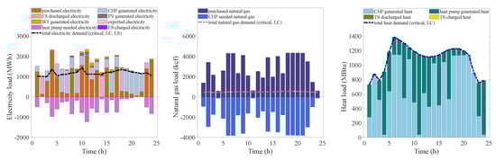
Figure 6.
Operational results of microgrid 1.
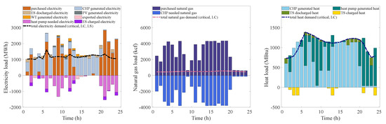
Figure 7.
Operational results of microgrid 2.
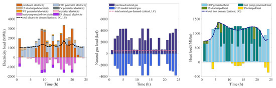
Figure 8.
Operational results of microgrid 3.
Table 8.
ES and TS results for microgrid 2. – : Not applicable.
Table 9.
ES and TS results for microgrid 3. – : Not applicable.
In addition, Table 8 and Table 9 indicate that increasing the rated capacity and power from microgrids 2 to 3 boosts ES and TS usage. Specifically, the total ES charging and discharging power in microgrid 2 are 1432.14 MW/h and 1292.46 MW/h, which are less than 1800.00 MW/h and 1624.45 MW/h in microgrid 3. A similar pattern happens to TS energy management (i.e., 1050.57 MBtu/h and 948.05 MBtu/h compared to 1264.09 MBtu/h and 1140.75 MBtu/h). Moreover, Table 10 shows the operational cost of three different microgrids. With ES and TS, microgrids 2 and 3 can reduce operational costs by 2.02% and 4.14% compared to microgrid 1, respectively. Furthermore, following the rise of ES and TS usage from microgrid 2 to 3, the operational costs of microgrids decrease notably. This is because microgrids with higher rated capacity and power of ES and TS are more capable of managing energy and reducing the potential cost.
Table 10.
Operational costs of microgrids.
5. Conclusions
In this study, a customised multi-energy pricing scheme is proposed for an energy retailer that manages multiple microgrids equipped with energy converters, storage, RES and DR programs. The proposed pricing problem is formulated as a bilevel optimisation model. The energy retailer is the leader at the upper level to maximise profit. Each multi-energy microgrid acting as a follower minimises the operational cost at the lower level. In addition, three hybrid metaheuristic algorithms (i.e., PSO, GA and SA) coordinated with the MILP program are developed to solve the model efficiently. Through numerical analyses, the GA-based hybrid solution algorithm is proved to have the best performance against others. The customised pricing scheme presents superiority compared to the uniform pricing scheme. In addition, since increasing the rated capacity and power of the ES and TS can improve the microgrids’ energy management capability, the retailer’s profit and microgrids’ operational costs reduce accordingly.
For future work, we would like to develop a machine learning or data-driven model at the lower level to present the interaction between the upper-level energy retailer’s price signals and the lower-level microgrids’ energy management decisions. The method will benefit real-world applications due to the existence of imperfect information of lower-level agents, such as microgrids and aggregators (that is, their operation models may not be known by retailers). In addition, we will consider developing an approximation and numerical approach for solving the bilevel model with the binary variables in the lower-level problem. The comparison between the approach and the aforementioned hybrid metaheuristic algorithms will also be studied. Furthermore, since environmental factors, such as carbon cost/budget, are increasingly implemented by different organisations (e.g. microgrids or local energy communities) as required by retailers and governments, it could affect retailers’ pricing decisions. Therefore, the objective functions and constraints of the bilevel model will consider such environmental factors in our future work. Lastly, we will investigate our modelling alternatives, such as cooperative game theory and bargaining mechanism, to model the interactions between the retailer and customers/microgrids.
Author Contributions
Conceptualization, F.M.; Methodology, Q.H. and F.M.; Software, Q.H.; Validation, Q.H.; Investigation, J.L.; Data curation, Q.H.; Writing—original draft, Q.H.; Writing—review & editing, F.M. and J.L.; Supervision, F.M. All authors have read and agreed to the published version of the manuscript.
Funding
This research received no external funding.
Data Availability Statement
No new data were created or analyzed in this study. Data sharing is not applicable to this article.
Conflicts of Interest
The authors declare no conflict of interest.
Nomenclature
| Abbreviations and Indices | |
| RES | Renewable energy sources |
| DR | Demand response |
| PSO | Particle swarm optimisation |
| GA | Genetic algorithm |
| SA | Simulated annealing |
| MILP | Mixed-integer linear program |
| DERs | Distributed energy resources |
| RTP | Real-time pricing |
| TOU | Time of use |
| EVs | Electric vehicles |
| CVaR | Conditional value at risk |
| EPEC | Equilibrium problem with equilibrium constraints |
| IESP | Integrated energy service provider |
| KKT | Karush–Kuhn–Tucker |
| CHP | Combined heat and power |
| ES, TS | Electrical storage, thermal storage |
| LC, LS | Load curtailment, load shifting |
| PV, WT | Photovoltaic, wind turbine |
| i | Index of microgrids |
| a | Index of households participating in load-shifting program |
| t | Index of time periods |
| Sets | |
| Set of microgrids | |
| Set of scheduling hours | |
| Set of households participating in load-shifting program | |
| Parameters | |
| Proportion that the electricity price sold by the microgrid i back to the retailer against the retail price. | |
| Operation and maintenance costs for CHP and heat pump in microgrid i. | |
| Start-up and shut-down costs of CHP and heat pump in microgrid i. | |
| Electrical and thermal storage costs. | |
| Load curtailment cost of electricity, natural gas and heat in microgrid i. | |
| Natural gas to electricity and electricity to heat conversion efficiency of the CHP in microgrid i. | |
| Minimum and maximum electricity volume generated by the CHP in microgrid i. | |
| Initial electricity volume and status of the CHP in microgrid i. | |
| Ramp-up and ramp-down limits of the CHP in microgrid i. | |
| Electricity to heat conversion efficiency of the Heat pump in microgrid i. | |
| Minimum and maximum heat volume generated by the heat pump in microgrid i. | |
| Initial heat volume and status of the heat pump in microgrid i. | |
| Ramp-up and ramp-down limits of the heat pump in microgrid i. | |
| Initial energy level of ES in microgrid i. | |
| ES charging, discharging and self-discharging rate in microgrid i. | |
| Minimum and maximum of the ES energy level in microgrid i. | |
| Minimum and maximum of the ES charging and discharging volume in microgrid i. | |
| Initial energy level of TS in microgrid i. | |
| TS charging, discharging and self-discharging rate in microgrid i. | |
| Minimum and maximum of the TS energy level in microgrid i. | |
| Minimum and maximum of the TS charging and discharging volume in microgrid i. | |
| Minimum and maximum electricity curtailment rate in microgrid i. | |
| Minimum and maximum natural gas curtailment rate in microgrid i. | |
| Minimum and maximum heat curtailment rate in microgrid i. | |
| Shiftable load adjustable time window of the household a in microgrid i. | |
| Start and stop time of the load-shifting program of the household a in microgrid i. | |
| Minimum and maximum of the shiftable load of the household a in microgrid i. | |
| Total electricity consumption of the household a in microgrid i during the load shifting program. | |
| Minimum and maximum of the PV-generated electricity volume in microgrid i at time t. | |
| Minimum and maximum of the wind turbine-generated electricity volume in microgrid i at time t. | |
| Spinning reserve ratio. | |
| Minimum and maximum of electricity volume that the microgrid i purchased from the retailer at time t. | |
| Minimum and maximum of electricity volume that the microgrid i sold to the retailer at time t. | |
| Total electricity and natural gas volume that the retailer purchased from the wholesale energy markets. | |
| Minimum and maximum of retail electricity price for microgrid i. | |
| Minimum and maximum of retail natural gas price for microgrid i. | |
| Average retail electricity and natural gas price over the scheduling hours. | |
| Variables | |
| Electricity and natural gas volume that the microgrid i purchased from the retailer at time t. | |
| Electricity volume that the microgrid i exports to the retailer at time t. | |
| Retail electricity and natural gas price for the microgrid i at time t. | |
| Electricity and heat volume generated by the CHP in microgrid i at time t. | |
| Natural gas volume that consumed by the CHP in microgrid i at time t. | |
| CHP operational, start-up and shut-down status in microgrid i at time t. | |
| Electricity consumed and heat generated by the heat pump in microgrid i at time t. | |
| Heat pump operational, start-up and shut-down status in microgrid i at time t. | |
| ES energy level in microgrid i at time t. | |
| ES charging and discharging volume in microgrid i at time t. | |
| ES charging and discharging status in microgrid i at time t. | |
| The final energy level of the ES in microgrid i. | |
| TS energy level in microgrid i at time t. | |
| TS charging and discharging volume in microgrid i at time t. | |
| TS charging and discharging status in microgrid i at time t. | |
| The final energy level of the TS in microgrid i. | |
| Electricity, natural gas and heat curtailment rate in microgrid i at time t. | |
| Operational status of the household a in microgrid i at time t. | |
| Shiftable load of the household a in microgrid i at time t. | |
| Electricity generated by PV and wind turbine in microgrid i at time t. | |
| Electricity importing and exporting status in microgrid i at time t. |
Appendix A. Input Data
Table A1.
Base energy demand for microgrid 1–3.
Table A1.
Base energy demand for microgrid 1–3.
| Time (h) | Microgrid 1 | Microgrid 2 | Microgrid 3 | ||||||
|---|---|---|---|---|---|---|---|---|---|
| Electricity (MWh) | Natural Gas (kcf) | Heat (MBtu) | Electricity (MWh) | Natural Gas (kcf) | Heat (MBtu) | Electricity (MWh) | Natural Gas (kcf) | Heat (MBtu) | |
| 1 | 842.92 | 387.74 | 519.30 | 504.00 | 210.00 | 554.40 | 622.31 | 311.16 | 715.66 |
| 2 | 828.44 | 381.08 | 531.32 | 499.20 | 208.00 | 549.12 | 596.93 | 298.46 | 686.46 |
| 3 | 820.95 | 377.64 | 578.56 | 504.00 | 210.00 | 554.40 | 580.13 | 290.06 | 667.14 |
| 4 | 831.32 | 382.41 | 698.73 | 499.20 | 208.00 | 549.12 | 580.06 | 290.03 | 667.07 |
| 5 | 861.44 | 396.26 | 972.46 | 508.80 | 212.00 | 559.68 | 597.68 | 298.84 | 687.33 |
| 6 | 924.58 | 425.31 | 1176.48 | 518.40 | 216.00 | 570.24 | 629.41 | 314.71 | 723.82 |
| 7 | 939.25 | 432.06 | 1137.13 | 528.00 | 220.00 | 580.80 | 677.44 | 338.72 | 779.05 |
| 8 | 981.48 | 451.48 | 1091.99 | 696.00 | 290.00 | 765.60 | 725.28 | 362.64 | 834.07 |
| 9 | 956.98 | 440.21 | 1032.92 | 835.20 | 348.00 | 918.72 | 770.57 | 385.29 | 886.16 |
| 10 | 937.68 | 431.33 | 979.94 | 936.00 | 390.00 | 1029.60 | 825.62 | 412.81 | 949.46 |
| 11 | 935.63 | 430.39 | 936.56 | 998.40 | 416.00 | 1098.24 | 879.69 | 439.85 | 1011.64 |
| 12 | 919.00 | 422.74 | 911.10 | 1008.00 | 420.00 | 1108.80 | 928.89 | 464.45 | 1068.23 |
| 13 | 916.53 | 421.60 | 900.55 | 1003.20 | 418.00 | 1103.52 | 968.60 | 484.30 | 1113.89 |
| 14 | 934.69 | 429.96 | 910.40 | 998.40 | 416.00 | 1098.24 | 998.55 | 499.28 | 1148.33 |
| 15 | 961.06 | 442.09 | 929.05 | 1008.00 | 420.00 | 1108.80 | 1018.46 | 509.23 | 1171.23 |
| 16 | 1002.37 | 461.09 | 968.73 | 1017.60 | 424.00 | 1119.36 | 1034.82 | 517.41 | 1190.04 |
| 17 | 1075.71 | 494.83 | 1004.19 | 1070.40 | 446.00 | 1177.44 | 1038.35 | 519.17 | 1194.10 |
| 18 | 1090.57 | 501.66 | 1017.83 | 1027.20 | 428.00 | 1129.92 | 1016.55 | 508.27 | 1169.03 |
| 19 | 1074.07 | 494.07 | 1016.88 | 619.20 | 258.00 | 681.12 | 978.60 | 489.30 | 1125.39 |
| 20 | 1046.70 | 481.48 | 985.27 | 614.40 | 256.00 | 675.84 | 943.57 | 471.79 | 1085.11 |
| 21 | 1011.72 | 465.39 | 887.76 | 590.40 | 246.00 | 649.44 | 900.10 | 450.05 | 1035.12 |
| 22 | 968.94 | 445.71 | 686.22 | 489.60 | 204.00 | 538.56 | 831.58 | 415.79 | 956.32 |
| 23 | 885.73 | 407.44 | 541.79 | 470.40 | 196.00 | 517.44 | 762.76 | 381.38 | 877.18 |
| 24 | 871.34 | 400.82 | 578.48 | 508.80 | 212.00 | 559.68 | 704.32 | 352.16 | 809.97 |
Table A2.
CHP parameters.
Table A2.
CHP parameters.
| Parameter | Value |
|---|---|
| Gas-to-power conversion rate | 0.3 |
| Power-to-heat conversion rate | 1 |
| Minimum power output (MW/h) | 40 |
| Maximum power output (MW/h) | 1200 |
| Ramp-up rate (MW/h) | 600 |
| Ramp-down rate (MW/h) | 600 |
| Operation & maintenance cost ($/kcf) | 15 |
| Start-up & shut-down cost ($) | 3.48 |
Table A3.
Heat pump parameters.
Table A3.
Heat pump parameters.
| Parameter | Value |
|---|---|
| Power-to-heat conversion rate | 0.9 |
| Minimum heat output (MBtu/h) | 20 |
| Maximum heat output (MBtu/h) | 1200 |
| Ramp-up rate (MBtu/h) | 600 |
| Ramp-down rate (MBtu/h) | 600 |
| Operation & maintenance cost ($/MW) | 2 |
| Start-up & shut-down cost ($) | 3 |
Table A4.
Maximum power of RES.
Table A4.
Maximum power of RES.
| Time (h) | PV Power (MW/h) | Wind Power (MW/h) |
|---|---|---|
| 1 | 0.00 | 0.00 |
| 2 | 0.00 | 0.00 |
| 3 | 0.00 | 0.00 |
| 4 | 0.00 | 0.00 |
| 5 | 0.00 | 0.00 |
| 6 | 6.43 | 0.00 |
| 7 | 35.50 | 0.00 |
| 8 | 67.44 | 5.98 |
| 9 | 80.50 | 41.53 |
| 10 | 114.05 | 77.96 |
| 11 | 127.20 | 135.86 |
| 12 | 63.41 | 165.05 |
| 13 | 47.74 | 94.61 |
| 14 | 48.03 | 145.59 |
| 15 | 39.42 | 71.58 |
| 16 | 34.44 | 88.22 |
| 17 | 13.96 | 45.99 |
| 18 | 1.92 | 41.53 |
| 19 | 0.00 | 18.38 |
| 20 | 0.00 | 13.05 |
| 21 | 0.00 | 2.55 |
| 22 | 0.00 | 1.55 |
| 23 | 0.00 | 0.56 |
| 24 | 0.00 | 0.00 |
Table A5.
Load-shifting program parameters.
Table A5.
Load-shifting program parameters.
| Shiftable Load | Total Energy (MWh) | Min. Power (MW/h) | Max. Power (MW/h) | Time Window (h) | Duration (h) |
|---|---|---|---|---|---|
| Task 1 | 250 | 25 | 150 | 2-18 | 5 |
| Task 2 | 110 | 5 | 50 | 2-20 | 8 |
| Task 3 | 180 | 20 | 80 | 5-22 | 6 |
| Task 4 | 150 | 10 | 60 | 3-21 | 12 |
| Task 5 | 200 | 15 | 100 | 8-22 | 10 |
Tasks 1–5 can be assigned to many appliances, such as dishwashers, electric vehicles and water heaters.
Table A6.
Wholesale electricity and natural gas prices.
Table A6.
Wholesale electricity and natural gas prices.
| Time (h) | Electricity Price ($/MWh) | Natural Gas Price ($/kcf) |
|---|---|---|
| 1 | 67.09 | 16.93 |
| 2 | 66.89 | 16.60 |
| 3 | 67.64 | 15.75 |
| 4 | 68.64 | 16.85 |
| 5 | 69.54 | 20.54 |
| 6 | 70.16 | 21.30 |
| 7 | 71.34 | 22.15 |
| 8 | 71.04 | 22.60 |
| 9 | 71.41 | 23.77 |
| 10 | 71.61 | 23.73 |
| 11 | 71.23 | 23.93 |
| 12 | 71.17 | 23.75 |
| 13 | 70.88 | 20.25 |
| 14 | 71.10 | 20.25 |
| 15 | 71.52 | 20.48 |
| 16 | 72.27 | 24.50 |
| 17 | 72.82 | 24.65 |
| 18 | 73.15 | 25.00 |
| 19 | 72.56 | 24.60 |
| 20 | 71.19 | 24.43 |
| 21 | 70.42 | 20.53 |
| 22 | 70.16 | 17.98 |
| 23 | 69.36 | 17.88 |
| 24 | 66.92 | 17.18 |
References
- Liu, P.; Ding, T.; Zou, Z.; Yang, Y. Integrated demand response for a load serving entity in multi-energy market considering network constraints. Appl. Energy 2019, 250, 512–529. [Google Scholar] [CrossRef]
- Mancarella, P. MES (multi-energy systems): An overview of concepts and evaluation models. Energy 2014, 65, 1–17. [Google Scholar] [CrossRef]
- Meng, F.; Ma, Q.; Liu, Z.; Zeng, X.J. Multiple dynamic pricing for demand response with adaptive clustering-based customer segmentation in smart grids. Appl. Energy 2023, 333, 120626. [Google Scholar] [CrossRef]
- Yang, J.; Zhao, J.; Luo, F.; Wen, F.; Dong, Z.Y. Decision-making for electricity retailers: A brief survey. IEEE Trans. Smart Grid 2017, 9, 4140–4153. [Google Scholar] [CrossRef]
- Aljohani, T.M.; Ebrahim, A.F.; Mohammed, O.A. Dynamic real-time pricing mechanism for electric vehicles charging considering optimal microgrids energy management system. IEEE Trans. Ind. Appl. 2021, 57, 5372–5381. [Google Scholar] [CrossRef]
- Nojavan, S.; Zare, K. Optimal energy pricing for consumers by electricity retailer. Int. J. Electr. Power Energy Syst. 2018, 102, 401–412. [Google Scholar] [CrossRef]
- Ghasemi, A.; Monfared, H.J.; Loni, A.; Marzband, M. CVaR-based retail electricity pricing in day-ahead scheduling of microgrids. Energy 2021, 227, 120529. [Google Scholar] [CrossRef]
- Su, S.; Li, Z.; Jin, X.; Yamashita, K.; Xia, M.; Chen, Q. Bi-level energy management and pricing for community energy retailer incorporating smart buildings based on chance-constrained programming. Int. J. Electr. Power Energy Syst. 2022, 138, 107894. [Google Scholar] [CrossRef]
- Hong, Q.; Meng, F.; Liu, J.; Bo, R. A bilevel game-theoretic decision-making framework for strategic retailers in both local and wholesale electricity markets. Appl. Energy 2023, 330, 120311. [Google Scholar] [CrossRef]
- Wei, C.; Wu, Q.; Xu, J.; Wang, Y.; Sun, Y. Bi-level retail pricing scheme considering price-based demand response of multi-energy buildings. Int. J. Electr. Power Energy Syst. 2022, 139, 108007. [Google Scholar] [CrossRef]
- Zhang, L.; Gao, Y.; Zhu, H.; Tao, L. Bi-level stochastic real-time pricing model in multi-energy generation system: A reinforcement learning approach. Energy 2022, 239, 121926. [Google Scholar] [CrossRef]
- Zeng, F.; Bie, Z.; Liu, S.; Yan, C.; Li, G. Trading model combining electricity, heating, and cooling under multi-energy demand response. J. Mod. Power Syst. Clean Energy 2019, 8, 133–141. [Google Scholar] [CrossRef]
- Wang, H.; Wang, C.; Sun, W.; Khan, M.Q. Energy Pricing and Management for the Integrated Energy Service Provider: A Stochastic Stackelberg Game Approach. Energies 2022, 15, 7326. [Google Scholar] [CrossRef]
- Zhu, X.; Sun, Y.; Yang, J.; Dou, Z.; Li, G.; Xu, C.; Wen, Y. Day-ahead energy pricing and management method for regional integrated energy systems considering multi-energy demand responses. Energy 2022, 251, 123914. [Google Scholar] [CrossRef]
- Yazdani-Damavandi, M.; Neyestani, N.; Shafie-khah, M.; Contreras, J.; Catalao, J.P. Strategic behavior of multi-energy players in electricity markets as aggregators of demand side resources using a bi-level approach. IEEE Trans. Power Syst. 2017, 33, 397–411. [Google Scholar] [CrossRef]
- Sinha, A.; Malo, P.; Deb, K. A review on bilevel optimization: From classical to evolutionary approaches and applications. IEEE Trans. Evol. Comput. 2017, 22, 276–295. [Google Scholar] [CrossRef]
- Yuan, G.; Gao, Y.; Ye, B.; Huang, R. Real-time pricing for smart grid with multi-energy microgrids and uncertain loads: A bilevel programming method. Int. J. Electr. Power Energy Syst. 2020, 123, 106206. [Google Scholar] [CrossRef]
- Sheha, M.; Mohammadi, K.; Powell, K. Solving the duck curve in a smart grid environment using a non-cooperative game theory and dynamic pricing profiles. Energy Convers. Manag. 2020, 220, 113102. [Google Scholar] [CrossRef]
- Li, B.; Roche, R.; Paire, D.; Miraoui, A. A price decision approach for multiple multi-energy-supply microgrids considering demand response. Energy 2019, 167, 117–135. [Google Scholar] [CrossRef]
- Yuan, G.; Gao, Y.; Ye, B.; Liu, Z. A bilevel programming approach for real-time pricing strategy of smart grid considering multi-microgrids connection. Int. J. Energy Res. 2021, 45, 10572–10589. [Google Scholar] [CrossRef]
- Qian, L.P.; Zhang, Y.J.A.; Huang, J.; Wu, Y. Demand response management via real-time electricity price control in smart grids. IEEE J. Sel. Areas Commun. 2013, 31, 1268–1280. [Google Scholar] [CrossRef]
- Meng, F.L.; Zeng, X.J. A Stackelberg game-theoretic approach to optimal real-time pricing for the smart grid. Soft Comput. 2013, 17, 2365–2380. [Google Scholar] [CrossRef]
- Meng, F.L.; Zeng, X.J. A profit maximization approach to demand response management with customers behavior learning in smart grid. IEEE Trans. Smart Grid 2015, 7, 1516–1529. [Google Scholar] [CrossRef]
- Meng, F.; Kazemtabrizi, B.; Zeng, X.J.; Dent, C. An optimal differential pricing in smart grid based on customer segmentation. In Proceedings of the 2017 IEEE PES Innovative Smart Grid Technologies Conference Europe (ISGT-Europe), IEEE, Torino, Italy, 26–29 September 2017; pp. 1–6. [Google Scholar]
- Yang, J.; Zhao, J.; Wen, F.; Dong, Z.Y. A framework of customizing electricity retail prices. IEEE Trans. Power Syst. 2017, 33, 2415–2428. [Google Scholar] [CrossRef]
- Yang, J.; Zhao, J.; Wen, F.; Dong, Z. A model of customizing electricity retail prices based on load profile clustering analysis. IEEE Trans. Smart Grid 2018, 10, 3374–3386. [Google Scholar] [CrossRef]
- Dai, Y.; Sun, X.; Qi, Y.; Leng, M. A real-time, personalized consumption-based pricing scheme for the consumptions of traditional and renewable energies. Renew. Energy 2021, 180, 452–466. [Google Scholar] [CrossRef]
- Huang, T.; Sun, Y.; Jiao, M.; Liu, Z.; Hao, J. Bilateral energy-trading model with hierarchical personalized pricing in a prosumer community. Int. J. Electr. Power Energy Syst. 2022, 141, 108179. [Google Scholar] [CrossRef]
- Dempe, S.; Zemkoho, A. Bilevel optimization. In Springer Optimization and Its Applications; Springer: Berlin/Heidelberg, Germany, 2020; Volume 161. [Google Scholar]
- Zhang, Y.; Meng, F.; Wang, R.; Kazemtabrizi, B.; Shi, J. Uncertainty-resistant stochastic MPC approach for optimal operation of CHP microgrid. Energy 2019, 179, 1265–1278. [Google Scholar] [CrossRef]
- Zhang, Y.; Meng, F.; Wang, R. A comprehensive MPC based energy management framework for isolated microgrids. In Proceedings of the 2017 IEEE PES Innovative Smart Grid Technologies Conference Europe (ISGT-Europe), IEEE, Torino, Italy, 26–29 September 2017; pp. 1–6. [Google Scholar]
- Zugno, M.; Morales, J.M.; Pinson, P.; Madsen, H. A bilevel model for electricity retailers’ participation in a demand response market environment. Energy Econ. 2013, 36, 182–197. [Google Scholar] [CrossRef]
- Kennedy, J.; Eberhart, R. Particle swarm optimization. In Proceedings of the Proceedings of the ICNN’95-International Conference on Neural Networks, IEEE, Perth, WA, Australia, 27 November–1 December 1995; Volume 4, pp. 1942–1948. [Google Scholar]
- Zhang, G.; Zhang, G.; Gao, Y.; Lu, J. Competitive strategic bidding optimization in electricity markets using bilevel programming and swarm technique. IEEE Trans. Ind. Electron. 2010, 58, 2138–2146. [Google Scholar] [CrossRef]
- Parsopoulos, K.E.; Vrahatis, M.N. Particle swarm optimization method for constrained optimization problems. Intell. Technol.—Theory Appl. New Trends Intell. Technol. 2002, 76, 214–220. [Google Scholar]
- Innocente, M.S.; Sienz, J. Constraint-handling techniques for particle swarm optimization algorithms. arXiv 2021, arXiv:2101.10933. [Google Scholar]
- Whitley, D. A genetic algorithm tutorial. Stat. Comput. 1994, 4, 65–85. [Google Scholar] [CrossRef]
- Van Laarhoven, P.J.; Aarts, E.H. Simulated annealing. In Simulated Annealing: Theory and Applications; Springer: Berlin/Heidelberg, Germany, 1987; pp. 7–15. [Google Scholar]
- PJM Data Directory. Available online: https://dataminer2.pjm.com/list (accessed on 10 November 2022).
- Department for Education Gas and Electricity Half Hourly Data. Available online: https://www.data.gov.uk/dataset/fee711fd-b405-4939-8945-5f9189839ad0/department-for-education-gas-and-electricity-half-hourly-data (accessed on 10 November 2022).
- Open Power System Data: When2Heat Heating Profiles. Available online: https://data.open-power-system-data.org/when2heat/2019-08-06 (accessed on 10 November 2022).
- Photovoltaic Geographical Information System. Available online: https://re.jrc.ec.europa.eu/pvg_tools/en/ (accessed on 12 November 2022).
- Smart Meters in London. Available online: https://www.kaggle.com/datasets/jeanmidev/smart-meters-in-london?select=weather_hourly_darksky.csv (accessed on 12 November 2022).
- Qi, S.; Wang, X.; Li, X.; Qian, T.; Zhang, Q. Enhancing integrated energy distribution system resilience through a hierarchical management strategy in district multi-energy systems. Sustainability 2019, 11, 4048. [Google Scholar] [CrossRef]
Disclaimer/Publisher’s Note: The statements, opinions and data contained in all publications are solely those of the individual author(s) and contributor(s) and not of MDPI and/or the editor(s). MDPI and/or the editor(s) disclaim responsibility for any injury to people or property resulting from any ideas, methods, instructions or products referred to in the content. |
© 2023 by the authors. Licensee MDPI, Basel, Switzerland. This article is an open access article distributed under the terms and conditions of the Creative Commons Attribution (CC BY) license (https://creativecommons.org/licenses/by/4.0/).