Abstract
The design and implementation of efficient photovoltaic (PV) plants and wind farms require a precise analysis and definition of specifics in the region of interest. Reliable Artificial Intelligence (AI) models can recognize long-term spatial and temporal variability, including anomalies in solar and wind patterns, which are necessary to estimate the generation capacity and configuration parameters of PV panels and wind turbines. The proposed 24 h planning of renewable energy (RE) production involves an initial reassessment of the optimal day data records based on the spatial pattern similarity in the latest hours and their follow-up statistical AI learning. Conventional measurements comprise a larger territory to allow the development of robust models representing unsettled meteorological situations and their significant changes from a comprehensive aspect, which becomes essential in middle-term time horizons. Differential learning is a new unconventionally designed neurocomputing strategy that combines differentiated modules composed of selected binomial network nodes as the output sum. This approach, based on solutions of partial differential equations (PDEs) defined in selected nodes, enables us to comprise high uncertainty in nonlinear chaotic patterns, contingent upon RE local potential, without an undesirable reduction in data dimensionality. The form of back-produced modular compounds in PDE models is directly related to the complexity of large-scale data patterns used in training to avoid problem simplification. The preidentified day-sample series are reassessed secondary to the training applicability, one by one, to better characterize pattern progress. Applicable phase or frequency parameters (e.g., azimuth, temperature, radiation, etc.) are related to the amplitudes at each time to determine and solve particular node PDEs in a complex form of the periodic sine/cosine components. The proposed improvements contribute to better performance of the AI modular concept of PDE models, a cable to represent the dynamics of complex systems. The results are compared with the recent deep learning strategy. Both methods show a high approximation ability in radiation ramping events, often in PV power supply; moreover, differential learning provides more stable wind gust predictions without undesirable alterations in day errors, namely in over-break frontal fluctuations. Their day average percentage approximation of similarity correlation on real data is 87.8 and 88.1% in global radiation day-cycles and 46.7 and 36.3% in wind speed 24 h. series. A parametric C++ executable program with complete spatial metadata records for one month is available for free to enable another comparative evaluation of the conducted experiments.
1. Introduction
The arrangements of PV and wind power systems are restricted by different topography and metrological conditions, seasonal variability, geographical constraints, short-term alterations, and intra-hour ramping of solar fluctuations and wind gusts. The non-stationarity of solar and wind parameters and their variations under specific atmospheric formations result in model insufficiency to provide adequate stand-alone estimation in an increased daily prediction horizon. Forecasting models based on AI are broadly designed in consideration of their granularity (related to ramping events and their variability) and operational control (including regularization in real power distribution, load scheduling and updated tracking in transmission units). Ensemble models, based on the aggregation of individual outputs, are basically made up of different groups, usually related to the pre-processing and learning/computing approaches [1]:
- General ensemble learning uses the assumption: single models contribute in specific ways to the overall prediction quality, i.e., a set of models is composed using the various approaches to improve the final AI accuracy.
- Cluster ensemble learning is primarily focused on data grouping, where outputs are categorized into several centers, which are supposed to accommodate input data samples with similar characteristics. Clustered data can be represented by linear/nonlinear functions whose model output estimations are aggregated in the final forecast. K-means is an unsupervised algorithm with variants that are generally applied in this approach.
- Decomposition ensemble learning multiresolution analysis is applied to decompose inputs into a meaningful pattern response to recognize time stationarity in data. Each component of the data is maintained and modeled separately to obtain the forecast aggregation as a sum output. High-frequency components are usually determined by non-linear data representation, whereas low-periodic signals are computed as linear functions. The most applicable techniques are based on wavelet decomposition at several levels, fused with a general AI regression.
- Evolutionary ensemble learning—the application of evolutionary algorithms in finding hybrid solutions for complex problems—can increase their efficiency in feature selection and parameter optimization in the output model fusion.
- Residual ensemble learning uses the presumption: radiation consists, in general, of two types of linear/nonlinear forms. A simple AI model is applied to linear components, while residuals are used in non-linear data representation. The overall forecast output is computed as the fusion of linear/non-linear models. Autoregressive moving average regression is commonly applied to linear data.
Statistical methods, which search for relationships in historical data records, offer simple and time-saving autonomous solutions compared to the complex atmospheric simulation of numerical systems. Hybrid AI algorithms combine data processing with model optimization for feature extraction and parameter adaptation. Singular analysis or empirical mode decomposition are the most common in forecasting procedures. Efficient data de-noising or component transformation can increase the forecasting accuracy and stability of hybrid models. Metaheuristics are effective in estimating initial training parameters and threshold limits if these cannot be defined otherwise. Non-negative constraint theory and the quasi-Newton algorithm can be used in AI learning [2]. Deep learning, based on long- and short-term memory or deep belief networks, can reduce some limitations of existing soft computing statistics by improving model performance, robustness, and stability [3].
Numerical Weather Prediction (NWP) models attempt to solve the physical evolutions of atmospheric processes at a specific scale, although the specific resolution of spatial data cannot be applied to a full temporal representation. Their increased resolution in spatial patterns has lower validity in the temporal representation applied in prediction, whereas their lower spatial pattern representation results in a high resolution in temporal data validity. NWP systems that use a low temporal representation in the data are applicable in short-time model simulations. The key drawback of physically-based NWP is the need to collect data from the specific local terrain. NWP systems produce point-by-point, 3D overall mathematical simulations of each meteorological factor (i.e., pressure, humidity, etc.). Their complexity requires many calculations and higher costs; therefore, they are more applicable in long-term forecasts [4]. Power curves can define a relationship between turbine or PV panel output power and weather variables, allowing easy transformation of the NWP solar or wind series into the RE forecast. Hybrid models that combine NWP with regression statistics or machine learning utilities based on cloud motion tracking perform best under unsettled conditions with higher uncertainties compared to standard single solutions [5].
Differential learning (DfL) is a novel neurocomputing approach, designed by the author, that is applied in all-day solar and wind quantity series statistical prediction 24 h ahead in a one-sequence computing procedure. DfL allows adequate modeling of complex and highly uncertain patterns included in weather datasets without significant simplification in their representation or dimensionality. It combines traditional numerical mathematics in the solution of simple PDEs defined and formed in binomial tree nodes using AI. Limitations of standard AI techniques can lead to casual failures in pattern breakover situations, which cannot usually be eliminated by standalone model statistics without NWP data processing or analysis. The previous forecasting models, published by the author, were based on adapted Similarity Theory (ST) and application of the Buckingham PI-theorem. The new presented DfL extends and elaborates on the previous concept by applying the Laplace transformation to PDE derivatives and the inverse operation in the restoration of original node functions in components, both based on operation calculus. The modular convergent combinations form a sum output. The step-by-step composition of the model was improved using several optimization and heuristic techniques (node input selection, combinatorial evolution, and gradient adaptation). The mathematical definition was also improved using several types of base substitution functions (rational, periodic, and power), which allow great variability in PDE solutions. DfL gradually extends its models by inserting the appropriate PDE components, produced one by one in a dynamically evolved parallel tree structure from node to node (starting empty). Substantial and incremental innovations, compared to the previous concept based on the fixed Neural Network (NN) architecture and ST [6], allow the formation of robust and reliable AI models that are adaptable and resistant to dynamical changes and chaotic incomputable instabilities.
2. Solar and Wind Quantities Forecasting—State of the Art
Freely provided NWP data (quantities of ground temperature with relative humidity, atm. pressure, visibility, wind, and descriptive weather type state) can be used in the 24-h irradiance prediction, as these forecasts are usually unavailable. Machine learning (ML) can predict irradiance and wind speed using different predictor variables from the reanalysis produced by the European Center for Medium-Range Weather Forecasting (ECMWF). The most relevant quantities of ECMWF datasets were selected using feature component analysis based on nearest-neighbor solutions [7]. The relationships between forecast data based on the mesoscale NWP model and the clearness index using Kalman filtering can be searched to improve the precision of the original NWP model in predicting day-to-day solar radiation [8]. ML based on utilities, which uses different combinations of inputs of selected meteorological data, can produce singular results in the refinement ensemble of solar radiation and wind speed forecasts, depending on the characteristics of the terrain, anomalies, and other conditions in particular regions [9].
Long-term memory (LSTM) networks can efficiently represent the relationships between historical day data in consecutive hours [10]. Weighted Gaussian Processing Regression (WGPR) can be used in multistep daily predictions of the main solar and wind components. The self-selection of valuable meta-data is performed using [11]:
- parallel structures
- WGPR cascades
Cluster-based learning can use K-means algorithms to obtain the intrinsic mode and residual components for each cluster. The weights are estimated in the final prediction of the ensemble model [12]. Daubechies wavelets can be used to recognize specific time-series components. Each meteorological input-output data sample is reduced to the detailed and approximate wavelet components. Their calculated first-level coefficients are used as model inputs to estimate the first-level output response. Analogously, this procedure is applied to the next levels of decomposition. Finally, all the approximate parameters of the computed output are used to construct estimates of the original variables [13]. The original solar and wind data can be itemized using intrinsic functions, and the residuals are calculated in the multivariate empirical mode decomposition. The selected elements are combined in the input vector to produce the multi-stage forecast model [14]. Data-driven models are based on identifying the appropriate inputs, although these are usually unavailable at all stations of a complex monitoring system. Satellite-derived predictors usually provide data for a hybrid AI modeling approach [15].
Satellite images can obtain high temporal resolution in comparison to the limited spatial resolution of ground-measured data, providing contrary high accuracy but significantly missing in some localities. Machine learning can improve spatial and temporal resolution, which is necessary for the adaptation of the model site, by searching for point-to-point relationships between satellite and ground-based data [16]. The spatial, temporal, spectral, and radiometric resolution of satellite instrumentation data allows presenting the current cloud spatial distribution, motion, or optical properties. These are directly related to the solar transient characteristics necessary in the detailed approximation of evolution in the cloud fields in consideration of advection processes. The information is used to evolve a transfer model that represents direct and diffuse solar insolation in both shadow and clear-sky structures [17].
Hybrid models are grouped into two main categories in consideration of their general strategies:
- ○
- Stacking-based learning
- ○
- Weighted ensembles
The stacking-based learning approach initially calculates forecasts of a few base models with single features, which are fed into the final high-level model. A weighted ensemble is easy to combine from several single weak model outputs. Probabilistic models allow for the representation of the uncertainty of outputs in terms of statistical distributions or prediction intervals. Parametric approaches usually assume that the prediction uncertainty is possible to describe by a probability distribution function. Non-parametric methods aim to generate prediction intervals that characterize the uncertainty of the calculated output. The original data set is usually first processed to identify outliers or reduce unwanted noise. Signal processing can decompose data series into different subseries that are applied as inputs in several models. The prediction results are then aggregated into the final product [18].
The proposed 24-h forecast optimization scheme covers:
- Day-ahead, timely forecasting in one-step sequence data processing
- Re-evaluation of training data items in the pre-estimated starting time range
- Formation of PDE models with the complexity related to training patterns
- Automatic selection of model inputs in the binary structure development
- Step-by-step PDE-component production by the parallel inserted binary-network nodes
- Re-adaptation of the component-sum model in each next prediction day
- Identification of unpredictable patterns in the statistical model verification test
3. Solar and Wind Quantities Daily Forecasting—Data and Methodology
Historical data records, applied in experiments, were first processed by auxiliary detection AI models. The evaluation test is based on the lowest errors calculated in the last 10 h with the gradually increased training range in 2…x days. This approach enables us to roughly estimate the applicable daytime periods in the evolution of statistical models. The first detected starting time at model initialization was first re-assessed taking into account a similarity coefficient. Pearson’s Correlation Distance (CD), calculated as the pattern Correlation Similarity (CS) Equation (1), can be used to gradually test and recognize, one by one, a particular suitable series of learning records.
P(p1 …, pn) and Q(q1 …, qn)-points in n-dimension data space cov(P,Q), var(P/Q)-covariance, variance in P, Q data vectors
Figure 1 illustrates the assignment of the roughly detected training record resulting from time-range initialization tests in the step-by-step increased validation periods of 2…x days. The applicable day-time intervals of selected data series were then secondarily reassessed, taking into account a defined similarity coefficient value calculated with respect to compared data samples in the latest corresponding day. If the initializing models are unable to compute acceptable testing errors in the latest sequenced data (induced by a passing front), the day-time range is randomly placed in the available data set to find the optimal learning base interval.
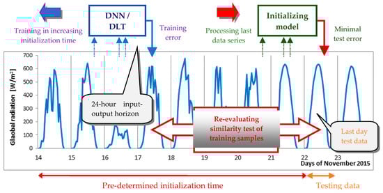
Figure 1.
First detection of the model initial time with reappraisal of data records, one-by-one.
Figure 2 illustrates the proposed prediction procedure applied in the development of solar and wind AI models in the absence of available NWP data. The resulting AI models were tested in the second stage for the latest data patterns to process the unlearned input data in computing the following solar or wind series in the corresponding time [19]. If the final models do not again obtain an acceptable threshold in testing errors, then their statistical results are apparently inapplicable and useless in prediction. Figure 3 gives a visualization of the ground location and scale distances of the airport observational and target RE production facilities. The airport observation station time in Luqa (+1 h) was necessary to synchronize with the western data recording time zone used in Tajoura, Djerba, and Monastir [20,21].
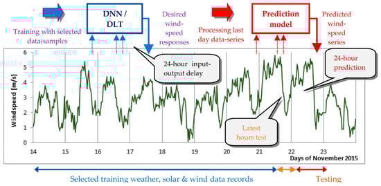
Figure 2.
Learning, testing, prediction practice in daily solar and wind parameter forecasting.
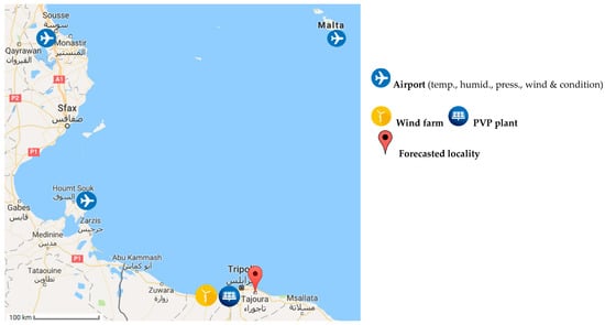
Figure 3.
The target solar- and wind-monitoring location in Tajoura with three supporting airport observational stations in the Mediterranean region.
Global (horizontal) radiation (GR), direct normal irradiance (DNI), and horizontal diffuse (HD) radiation were measured in a 1 min series, Equation (2) at the Tajoura Solar Energy Research Centre [20] from 1 to 30 November 2015. The minutely failure-free solar, wind speed (WS), and other weather norm data were averaged each 30 min. to match the reference recording time of free available meteorological station observations, mandatory at local airports. Some record series were missing from the historical sets of Djerba and Monastir airports and needed to be supplemented with approximate or interpolated data points in the lost half-hours [21]. Spatial data of standard weather quantities from a larger territory are inevitable in AI forecasting using a 24-h input-output time shift with no NWP processing series (Figure 3). Pattern changeovers or instabilities in boundary zones (e.g., storm cyclones or frontal waves), coming through the target position in the next day-hours, are incorporated into the multiscale forecasting model in advance to capture and reflect the progress of global relations [22].
GR = DNI + HD
GR = Global (horizontal) radiation, DNI = direct normal irradiance, HD = diffuse (horizontal) radiation [W/m2].
4. Computing Techniques Applied in Daily AI Model Development
4.1. Differential Learning—A New Hybrid Neuro-Math Computing Design
Differential learning (DfL) is a new soft-computing strategy, developed and designed by the author, which fuses several ML principles on a mathematical background, allowing the solution of partial differential equations. Differential neural networks (DNN) employ a hybrid AI-based computing approach using DfL and gradual model expansion principles. It itemizes and factorizes parametric PDE of n-variables and k-generalized order into simplified standard PDEs of recognized order Equation (3) using only reduction 2 inputs in included structural nodes. DNN can be used in modeling of chaotic and highly uncertain systems, whether physical or social, which include large numbers of data variables and are difficult to represent by linear equation definitions or computed next states by standard AI methods. The evolution of DNN models includes a self-determination of the most relevant variables from each of the two inputs to the nodes and their data transformation. This advanced AI procedure usually outperforms the traditional extraction of data features and signal processing. DNN evolves structures of polynomial neural network (PNN) models by inserting its nodes, one by one, into the multilayer binary tree, starting empty. Applicable nodes are determined and selected to form PDE-modular components included (or extracted) in (or from) the model sum series, which improves step by step its approximation ability for target data samples. A progressive expansion of the new modeling strategy allows us to form applicable model solutions based on Kurt Goedel’s incompleteness theorem. Step-by-step inserted nodes extend a DNN tree form using the proposed back-computing principles for multilayer PNNs. DNN processes the relevant data input to predetermine the specific node PDEs in the combinatorial iteration procedure according to adapted formulations based on Operation Calculus (OC). The order of polynomial substitution, determined by the modules of the DNN nodes, corresponds to the definition of PDE in its transformation and restoration [22].
A, B, …, G–parametric coefficients of x1, x2 independent variables for the unknown u(x1, x2) function
The OC transformation applied for all PDE derivatives of nth order of the f(t) function is stated in the preposition: each derivative is possible to substitute by its Laplace transform on supposed defined initial conditions, Equation (4).
f(t), f’(t), …, f(n)(t)–continuous t-time originals in <0+, ∞> F(p)-complex image of the function f(t) p, t-complex, and real variables→L{}–transformation.
The L transformed derivatives of a function f(t) define a set of standard linear algebraic equations, Equation (5), in which the complex p-valued transforms F(p) can be formulated and modified to pure rational components Equation (3).
B, C, Ak-coefficients of elementary fractions a,b-polynom. Parameters α1, α2, …, αk-simple real roots.
Separate ratio fractions are related to L-transformations of the original f(t) and it is possible to apply them in the inverse L-restoration in OC Equation (6) to obtain the initially defined PDE f(t) Equation (3).
P(p), Q(p)–multinomials of degree s-1, s→α1, α2, …, αn-simple real roots of Q(p) p–complex variable.
In the case where f(t) is of a periodic nature, then its derivative conversion takes the form of a sine/cosine circulator substitution, where the original is computed as the inverse L-restoration Equation (7). The sine/cosine extension formulation involves the amplitude and frequency of the data periods to define the node L-transform related to the substitution of these cycle characteristics in sub-PDEs.
γk–complex roots of Q(p) t–time variable.
The original inverse L-restoration is necessary to transform the rational Equation (6) or cycle form of the algebraic equations Equation (7), resulting from the initial formulation of PDEs. Two-variable originals uk are produced in selected DNN nodes (Figure 4) in the form of sum PDE modules for the decomposed n-variable function u (3).
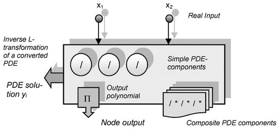
Figure 4.
Blocks define and solve sub-PDEs in the chosen DNN nodes of the modular model.
The complex conjugates in the Euler formulation c Equation (8) are determined by the expression of the original functions f(t) Equation (6). Radius r (data amplitude) is related to the rational form and phase calculated as = arctg(x2/x1) of the variables x1, x2 corresponds to the inverse restoration L of converts F (p).
φ–phase, r–radius, i–imaginary number, c–Euler’s complex number Key DNN features and innovations, allowing [23]:
- Parsing the n-parametric k-order PDE into a summary set of defined and converted PDEs
- Evolving Structures by Inserting Node by Node in the Back-Computing PNN Tree
- Self-composing autonomous PDE modules in nodes to be inserted into the sum model
- Various conversion types of PDEs based on OC-defined forms in its model representation
- L-transforming of node PDE derivatives and the OC inverse recovering searched originals
- Selection of applicable 2-inputs in nodes to extend/reduce the PDE-modular model
- Non-reducing substantially dimensions in data, yielding undesired model simplification
- Various combinatorial solutions in PDE node modules to represent data patterns
4.2. Matlab—Deep Learning Toolbox
Deep learning (DL) regression is a novel computing strategy that allows detailed modeling of patterns from time-lagged data. DL can employ extended neural net architectures of various types in multilayer forms to decompose input data relationships, not necessarily relying on a specifically designed computing approach. The Matlab Deep Learning Toolbox (DLT) includes a modeling framework and a graphical design tool for the implementation and application of DL neural algorithms. Its architecture applies a time-delayed network using the Long-Short-Term Memory (LSTM) approach in a sequence-to-sequence regression [24], including the following multilayer components:
- Sequence input data layer
- LSTM network
- Fully-connected layer
- Drop-out layer
- Fully-connected layer
- Regression output net layer
The most important component of DLT regression is usually the LSTM net. The sequence input layer supplies time series input for the LSTM layer. The LSTM learns deep, long-term relationships among sequenced data series in iterative time stages. LSTM blocks represent the actual current state (ct−1, ht−1) in the next time X for data sequences to compute the ht output (which means inner state) and update the cell ct state at time t (Figure 5). LSTM cells keep data information from previous times t−1, for the next update state. This information is preserved by hidden ht states (their output) and cell ct states. Drop-out layers set random inputs to zero (or other) values, applying defined probability functions to ensure model diversity. The loss of function is calculated as a gradient in relation to the predetermined batch size minima in the data subsets in the training procedure to obtain the optimal update values in weights.
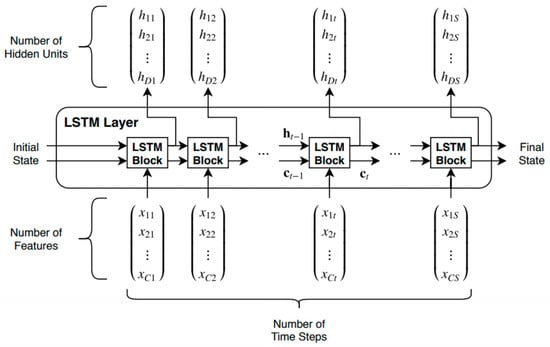
Figure 5.
Data flow chart in the processing and representation time series X with C feature channels of length S in an LSTM network.
DLT employs a form of LSTM net to form relevant pattern representations from input/output training data. Its architecture fuse multi-layer data processing based on standard operational and computational principles with elements biologically inspired by brain structures. The DLT computing framework includes an experimentally designed structure of replicated layers with convolution, dropout, and other types.
5. Data Experiments in Day-Ahead AI Solar and Wind Forecasting
Graphs in the demo Figure 6 and Figure 7 display the first-day real and estimate data series in day periods of 7–19 h irradiance and 24 h wind speed, respectively, computed by the AI statistics DNN and DLT models, including the complete 10-day comparative evaluation in an autumn season.
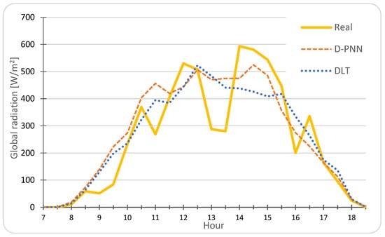
Figure 6.
14.11.2015, Tajoura City, solar-radiation prediction day RMSE: DNN = 89.22, DLT = 91.67 [W/m2].
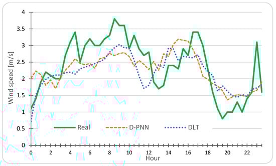
Figure 7.
14.11.2015, Tajoura City, wind-speed prediction day RMSE: DNN = 0.618, DLT = 0.598 [m/s].
The AI models can accurately approximate the ramping series of a target quantity in changing weather. The character of patterns in the next-day intervals remains unchanged, without significant changes in data involving an essential similarity in progress, as presented in the illustrative day graphs of Figure 6 and Figure 7. Significant breaks in night changes are apparent after 21 November in the form of new pattern characteristics (Figure 1 and Figure 2) that denote a type of sunny and gusty weather. The irradiation record series were standardized by means of the Clear Sky Index (CSI) in nondimensional expression to avoid the use of solar day-cycle-dependent data of the actual sun position about the horizon. CSI standardized data series are computed according to the pre-detected ideal “clear sky” maxima to allow estimates for any hour of day in every seasonal time without the use of absolute radiation data values. The GR data output is re-retrieved from the normal CSI estimate series considering the prediction time [25]. Periodic quantities (for example, GR, DNI, ground temperature, relative humidity, or direction of the wind) are self-recognized in the development of model structures and the selection of base functions. They are correlated with amplitudes at the corresponding times and are directly modeled in a cycle PDE conversion (7) by formulating model components [26].
6. Solar and Wind Daily AI Prediction Statistical Evaluation of Experiments
Figure 8 and Figure 9 summarize the avg. RMSE day errors of the two statistically evaluated AI computational models in forecasting solar radiation and wind speed 24 h ahead in the 10-day examination autumn season.
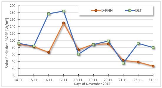
Figure 8.
10-day solar radiation avg. day prediction RMSE: DNN = 74.74, DLT = 99.04 [W/m2].
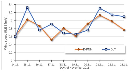
Figure 9.
10-day wind-speed avg. day prediction RMSE: DNN = 0.826, DLT = 0.925 [m/s].
An evident drop in irradiation on 16 November (Figure 1) results in an increase in the prediction RMSEs of both the examined DNN, DLT methods in the current and next two days. (Figure 8). A drastic change in the solar pattern from unsettled to sunny days on 21 November also results in difficulties in DL model development (data sample assignment) and a slight increase in errors. However, DNN‘s robust models succeed in eliminating this training handicap. On the other hand, the similarity of day patterns included in the short time period from 17 to 20 November allows for stable AI predictions with a small decrease in errors. Analogous significant differences between wind training/testing and prediction pattern characteristics (gust fluctuations) on 15 and 20 November (Figure 2) affect an accumulative increase in model errors (Figure 9) and lower prediction efficiency. DNN models again partially reduce the impact of unfavorable changes in conditions on AI prediction. Unacceptable increases in daily avg.forecast errors can be suppressed using more sophisticated selection algorithms when searching trainable record intervals Equation (1), according to detected frontal breaks in similar patterns in extended-monthly data sets. The quality of the model approximation usually depends on the optimal predetermination of training and testing sample sets and their applicability in relation to the character of pattern progress and eventual changeovers [22].
Figure 10 and Figure 11 compare Pearson’s correlation determination coefficient (PDC) for the day-independent DNN and DLT models applied to estimate the next 24-h series in their sequenced computation during the 10-day fall period. Both results from the AI day model statistics are more or less similar in GR forecating, while DNN considerably outperforms DLT in WS. The low-valued PDC alterations (even zero) of DLT indicate its undesirable averaging and less approximation ability in the computation of predicted WS output series as a result of uncertainty in gust variability. Each of the two applied AI modeling strategies gets a slight increase in PDC in an accurate approximation of the day GR cycle series, more than 24 h. forecasting unexpected short-term ramp variances in WS resulting in strong PDC alterations, which imply some instability and less reliability of the DLT models based on LSTM compared with the DNN (Figure 11).
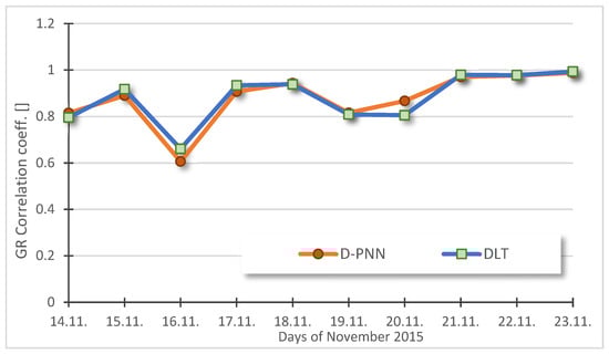
Figure 10.
10-day solar-radiation avg. prediction day Correlat. determin. coeff.: DNN = 0.878, DLT = 0.881 [].
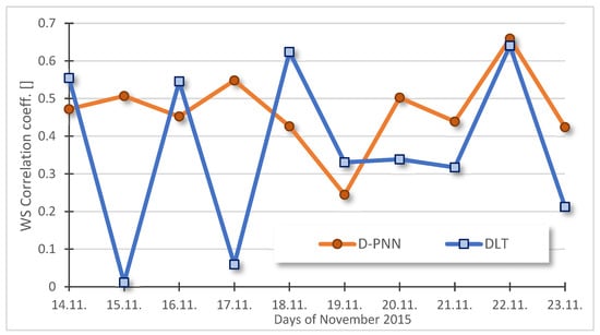
Figure 11.
10-day wind-speed avg. day prediction correlat. determination coeff.: DNN = 0.467, DLT = 0.363 [].
DNN node-by-node evolvement in its binary selective architecture composing step-by-step the additive expansion model allows incremental learning, i.e., inserting new or removing useless sum PDE-components in the model re-adjustment according to an updated training set without resetting the present structure and model output combination. Newly assigned day samples can be additionally learned to re-adapt the same D–PNN model for each new situation in the next partial training step, improving its robustness and stability for unknown prediction patterns and parameter uncertain variances. The complexity of modeling is gradually increased and refined to gain new knowledge, along with retaining previously learned skills. It requires efficient searching of a larger spatial data archive to detect applicable training samples and improve model/net-structure optimization.
Figure 12 and Figure 13 present the preliminary detected modeling initial time used in searching the start day according to the chosen similarity distance in the reconsideration of trainable sample data sequences.
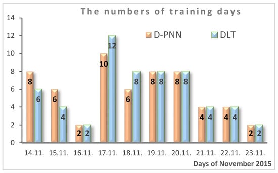
Figure 12.
The predetermined initial numbers of the trainable data day series are re-evaluated for selected pattern similarity in the development of solar radiation models.
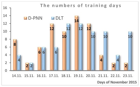
Figure 13.
The roughly pre-estimated initial numbers of the trainable day data series applied in the re-evaluation of selected pattern samples in the development of wind speed models.
The DNN computational complexity is naturally higher, as the model is gradually composed using node-by-node evolved binomial tree structures that produce acceptable sum PDE components, which can be included one by one in the output sum to decrease errors. Several optimization algorithms are to be synchronized to select the optimal 2-input nodes (to reduce combinatorial explosion) and convergent combinations of applicable modular components in recognition of PDE-substitution functions in model definition (rational, periodical, and power), elimination of redundant PDE-components (from the first included layers), parameter adaptation (gradient and back-propagation), etc. DNN is self-optimizing in all these automated procedures; that is, it does not require the estimation of training parameters or network structure (only the testing coefficients must be set experimentally). DLT uses a standard NN architecture and optimization, which requires a sophisticated hand-made design in the model structure, layer types, and learning parameters. The DNN model complexity is higher as usual in standard soft computing, corresponding to those of data patterns, which allows modeling and representation of high dynamic, chaotic, and uncertain (weather dependent) systems. Model oversimplification can result in strong failures in statistical prediction using traditional AI learning approaches. However, the computational complexity can differ on each prediction day, according to the trainability and similarity specifics of the applied patterns represented by the PDE modular models.
7. Discussion
Sudden variances in data patterns are predominantly the result of irregular ground-level airflow processes and additional chaotic turbulent instabilities. Many anomalies complicate the applicability of oscillating patterns in AI learning directly related to the 24-h fixed input time delay used to calculate the desired output in modeling and prediction [27]. Accurate 24-h estimation in data ramping events mainly corresponds to the optimized selective training intervals in similar weather periods. Dramatic unexpected changes in their patterns, which result in rapid short-time fluctuations in the GR or WS series, complicate AI prediction statistics and lead to model over failures (Figure 6). The proper re-consideration of approximate training data intervals (record by record) is dependent mainly on the optimal selection of similarity distance expressed in the terms of correlation parameters to relate patterns in n-dimensional data Equation (1). More sophisticated or fused approaches in the computation of the similarity measure will naturally yield adequate results in the better applicability of selected data samples. In the case of breaking frontal-day changes in weather patterns, GR or WS-trained data relations can absolutely differ from those expected in the forecasting hours. An experimentally predefined test threshold in computed errors may be applied considering the previously risen malfunctions in day-model estimations of forecasting series or compute a similarity parameter for the corresponding NWP data. Failing the statistical validation of AI models in the error output or the comparative NWP similarity testing, processing cloud cover data [21] is an additional alternative to obtain reliable GR + WS predictions [28]. Sudden night breaks in local patterns can be searched and identified algorithmically in big data observational record sets in the assessment of multiple initialize times, usable in successful training (Figure 10). An additional 24-h lagged data input usually improves the AI modeling accuracy, analogous to rel. humidity [29].
8. Conclusions
The proposed data sequence processing schemes for the daily prediction of statistical GR and WS were verified by applying two novel bioinspired computational strategies. The benefits of one-step all-day series estimation are clearly shown in the model efficiency and low time-consuming costs. Each day self-standing AI model is capable of providing complete GR and WS prediction series in all-day horizon, using the same input-output time shift in the sequence data computing. The applied iterative data processing strategy enables early forecasting in a day-horizon with the acceptable accuracy required in RE production planning. The AI results based on historical data statistics differ from the quality and reliability of intra-hourly or NWP solutions only in a slight measure, which was approved by the daily-performed experiment evaluation. This approach enables us to provide reliable early evening GR and WS prognoses without a computing delay, required in NWP data simulations, on a daily basis, which is vital in the planning and scheduling of power consumption in autonomous smart off-grid systems that rely on RE. The benefits of the physical approach employed in NWP data simulations are apparently shown in frontal breaks in patterns, where AI statistics using 24-h data output shifting are unreliable and the models may be completely out of date, flawed, and inapplicable for new data patterns in many situations. Specific time-delayed output models can be used to revise rough day-ahead prognoses of the more efficient and less time-consuming all-day iterative forecasting strategy in shorter-term horizons in doubtful cases, according to early change localization and state detection using NWP data comparative similarity analysis. Inconsistent AI model estimates in the next hours usually indicate lower reliability in the statistics prediction, where NWP data post-processing can stand for. The DNN models proved their computing stability and resistance to unpredictable, chaotic changes in pattern progress in AI learning and prediction on the mid-term horizon compared to DL.
Parametric C++ modeling software, including historical spatial solar, wind, and meteorological research/airport observational sets, is available in repositories to enable additional evaluation experiments in comparison with the presented forecasting results.
Funding
This work was supported by SGS, VSB-Technical University of Ostrava, Czech Republic, under the grant No.\ SP2023/12 ‘Parallel processing of Big Data X’.
Data Availability Statement
Data and parametric ++ software is available as the Ref. [23].
Conflicts of Interest
The authors declare no conflict of interests.
Abbreviations
AI = Artificial Intelligence, RE = Renewable Energy, PVP = Photo-Voltaic (PV) Power, NWP = Numerical Weather Prediction, WS = Wind Speed, ECMWF = European Centre for Medium Range Weather Forecasting, DNN = Differential Neural Network, DfL = Differential Learning, ML = Machine Learning, LSTM = Long-Short-Term Memory (network), DLT = Deep Learning Toolbox (of Matlab), WGPR = Weighted Gaussian Process Regression, OC = Operator Calculus, ST = Similarity Theory, GMDH = Group Method of Data Handling, PNN = Polynomial Neural Network, PDE = Partial Differential Equation, OC = Operator Calculus, L-transform = Laplace Transformation, CS = Correlation Similarity, CD = Correlation Distance, PDC = Pearson’s Determination Coefficient, GR = Global (horizontal) Radiation, DNI = Direct Normal Irradiance, HD = Horizontal Diffuse Radiation, Neuron = substituting fraction derivative term, CT = Composite Term, Block = node PDE solutions, CSI = Clear Sky Index, RMSE = Root Mean Square Error, NN = Neural Network.
References
- Guermoui, M.; Melgani, F.; Gairaa, K.; Mekhalfi, M.L. A comprehensive review of hybrid models for solar radiation forecasting. J. Clean. Prod. 2020, 258, 120357. [Google Scholar] [CrossRef]
- Yang, Z.; Wang, J. A combination forecasting approach applied in multistep wind speed forecasting based on a data processing strategy and an optimized artificial intelligence algorithm. Appl. Energy 2018, 230, 1108–1125. [Google Scholar] [CrossRef]
- Kumari, P.; Toshniwal, D. Deep learning models for solar irradiance forecasting: A comprehensive review. J. Clean. Prod. 2021, 318, 128566. [Google Scholar] [CrossRef]
- Bazionis, I.; Georgilakis, P. Review of Deterministic and Probabilistic Wind Power Forecasting: Models, Methods, and Future Research. Electricity 2021, 2, 13–47. [Google Scholar] [CrossRef]
- Blaga, R.; Sabadus, A.; Stefu, N.; Dughir, C.; Paulescu, M.; Badescu, V. A current perspective on the accuracy of incoming solar energy forecasting. Prog. Energy Combust. Sci. 2018, 70, 119–144. [Google Scholar] [CrossRef]
- Zjavka, L. Numerical weather prediction revisions using the locally trained differential polynomial network. Expert Syst. Appl. 2016, 44, 265–274. [Google Scholar] [CrossRef]
- Ghimire, S.; Deo, R.C.; Downs, N.J.; Raj, N. Global solar radiation prediction by ANN integrated with European Centre for medium range weather forecast fields in solar rich cities of Queensland Australia. J. Clean. Prod. 2019, 216, 288–310. [Google Scholar] [CrossRef]
- Che, Y.; Chen, L.; Zheng, J.; Yuan, L.; Xiao, F. A novel hybrid model of wrf and clearness index-based kalman filter for day-ahead solar radiation forecasting. Appl. Sci. 2019, 19, 3967. [Google Scholar] [CrossRef]
- Siva Krishna Rao K, D.V.; Premalatha, M.; Naveen, C. Analysis of different combinations of meteorological parameters in predicting the horizontal global solar radiation with ann approach: A case study. Renew. Sustain. Energy Rev. 2018, 91, 248–258. [Google Scholar] [CrossRef]
- Qing, X.; Niu, Y. Hourly day-ahead solar irradiance prediction using weather forecasts by LSTM. Energy 2018, 148, 461–468. [Google Scholar] [CrossRef]
- Guermoui, M.; Melgani, F.; Danilo, C. Multi-step ahead forecasting of daily global and direct solar radiation: A review and case study of ghardaia region. J. Clean. Prod. 2018, 201, 716–734. [Google Scholar] [CrossRef]
- Sun, S.; Wang, S.; Zhang, G.; Zheng, J. A decomposition-clustering-ensemble learning approach for solar radiation forecasting. Sol. Energy 2018, 163, 189–199. [Google Scholar] [CrossRef]
- Hussain, S.; AlAlili, A. A hybrid solar radiation modeling approach using wavelet multiresolution analysis and artificial neural networks. Appl. Energy 2017, 208, 540–550. [Google Scholar] [CrossRef]
- Prasad, R.; Kwan, P.; Ali, M.; Khan, H. Designing a multi-stage multivariate empirical mode decomposition coupled with ant colony optimization and random forest model to forecast monthly solar radiation. Appl. Energy 2017, 236, 778–792. [Google Scholar] [CrossRef]
- Ghimire, S.; Deo, R.C.; Raj, N.; Mi, J. Wavelet-based 3-phase hybrid SVR model trained with satellite-derived predictors, particle swarm optimization and maximum overlap discrete wavelet transform for solar radiation prediction. Renew. Sustain. Energy Rev. 2019, 113, 109–221. [Google Scholar] [CrossRef]
- Narvaez, G.; Giraldo, L.F.; Bressan, M.; Pantoja, A. Machine learning for site-adaptation and solar radiation forecasting. Renew. Energy 2017, 167, 333–342. [Google Scholar] [CrossRef]
- Miller, S.D.; Rogers, M.A.; Haynes, J.M.; Sengupta, M.; Heidinger, A.K. Short-term solar irradiance forecasting via satellite/model coupling. Sol. Energy 2018, 168, 102–117. [Google Scholar] [CrossRef]
- Wang, Y.; Zou, R.; Liu, F.; Zhang, L.; Liu, Q. A review of wind speed and wind power forecasting with deep neural networks. Appl. Energy 2021, 304, 117766. [Google Scholar] [CrossRef]
- Zjavka, L.; Misak, S. Direct Wind Power Forecasting Using a Polynomial Decomposition of the General Differential Equation. IEEE Trans. Sustain. Energy 2018, 9, 1529–1539. [Google Scholar] [CrossRef]
- The Centre for Solar Energy Research in Tajoura City, Libya. Available online: www.csers.ly/en (accessed on 15 January 2023).
- Weather Underground Historical Data Series: Luqa, Malta Weather History. Weather Underground (wunderground.com). Available online: www.wunderground.com/history/daily/mt/luqa/LMML (accessed on 15 January 2023).
- Zjavka, L. Photo-voltaic power daily predictions using expanding PDE sum models of polynomial networks based on Operational Calculus. Eng. Appl. Artif. Intell. 2020, 89, 103409. [Google Scholar] [CrossRef]
- DNN Application C++ Parametric Software Incl. Solar, Wind & Meteo-Data. Available online: https://drive.google.com/drive/folders/1ZAw8KcvDEDM-i7ifVe_hDoS35nI64-Fh?usp=sharing (accessed on 15 January 2023).
- Matlab—Deep Learning Tool-Box (DLT) for Sequence to Sequence Regressions. Available online: www.mathworks.com/help/deeplearning/ug/sequence-to-sequence-regression-using-deep-learning.html (accessed on 15 January 2023).
- Zjavka, L. Photo-voltaic power intra-day and daily statistical predictions using sum models composed from L-transformed PDE components in nodes of step by step developed polynomial neural networks. Electr. Eng. 2021, 103, 1183–1197. [Google Scholar] [CrossRef]
- Zjavka, L. Photovoltaic Energy All-Day and Intra-Day Forecasting Using Node by Node Developed Polynomial Networks Forming PDE Models Based on the L-Transformation. Energies 2021, 14, 7581. [Google Scholar] [CrossRef]
- Vannitsem, S. Dynamical Properties of MOS Forecasts: Analysis of the ECMWF Operational Forecasting System. Weather Forecast. 2008, 23, 1032–1043. [Google Scholar] [CrossRef]
- Zjavka, L.; Krömer, P.; Mišák, S.; Snášel, V. Modeling the photovoltaic output power using the differential polynomial network and evolutional fuzzy rules. Math. Model. Anal. 2017, 22, 78–94. [Google Scholar] [CrossRef]
- Zjavka, L.; Sokol, Z. Local improvements in numerical forecasts of relative humidity using polynomial solutions of general differential equations. Q. J. R. Meteorol. Soc. 2018, 144, 780–791. [Google Scholar] [CrossRef]
Disclaimer/Publisher’s Note: The statements, opinions and data contained in all publications are solely those of the individual author(s) and contributor(s) and not of MDPI and/or the editor(s). MDPI and/or the editor(s) disclaim responsibility for any injury to people or property resulting from any ideas, methods, instructions or products referred to in the content. |
© 2023 by the author. Licensee MDPI, Basel, Switzerland. This article is an open access article distributed under the terms and conditions of the Creative Commons Attribution (CC BY) license (https://creativecommons.org/licenses/by/4.0/).