Article

A Two-Terminal Fault Location Fusion Model of Transmission Line Based on CNN-Multi-Head-LSTM with an Attention Module

1
College of Electrical Engineering, Zhejiang University, Hangzhou 310027, China
2
Department of Electrical Engineering, School of Automation, Guangdong University of Technology, Guangzhou 510006, China
3
Brunel Interdisciplinary Power Systems Research Centre, Department of Electronic and Electrical Engineering, Brunel University London, London UB8 3PH, UK
*
Authors to whom correspondence should be addressed.
Energies 2023, 16(4), 1827; https://doi.org/10.3390/en16041827
Submission received: 21 December 2022 / Revised: 16 January 2023 / Accepted: 10 February 2023 / Published: 12 February 2023

Abstract

:
Most traditional artificial intelligence-based fault location methods are very dependent on fault signal selection and feature extraction, which is often based on prior knowledge. Further, these methods are usually very sensitive to line parameters and selected fault characteristics, so the generalization performance is poor and cannot be applied to different lines. In order to solve the above problems, this paper proposes a two-terminal fault location fusion model, which combines a convolutional neural network (CNN), an attention module (AM), and multi-head long short-term memory (multi-head-LSTM). First, the CNN is used to accomplish the self-extraction of fault data features. Second, the CBAM (convolutional block attention module) model is embedded into the convolutional neural network to selectively learn fault features autonomously. Furthermore, the LSTM is combined to learn the deep timing characteristics. Finally, a MLP output layer is used to determine the optimal weights to construct a fusion model based on the results of the two-terminal relative fault location model and then output the final location result. Simulation studies show that this method has a high location accuracy, does not require the design of complex feature extraction algorithms, and exhibits good generalization performance for lines with different parameters, which is of great importance for the development of AI-based methods of fault location.

1. Introduction

Transmission lines are located in the field with harsh outdoor operating environments, and faults occur frequently which may lead to long-term line outage. Identifying the accurate location of transmission line faults is very useful for quick fault recovery, which is of great significance to ensure the safety of power systems [1].
Traditional fault location methods are mainly divided into two categories: fault analysis method and traveling wave method [2,3,4,5]. The former includes the single-end method [6,7] and the double-end method [8] according to the data source. The fault distance can be obtained by solving the equation according to the relationship between voltage, current, and fault position, but is greatly affected by transition resistance and the transmission error of the transformer. The latter needs the support of hardware equipment, and its reliability cannot be guaranteed due to the difficulty of wavefront calibration [9].
In recent years, intelligent fault location methods have been introduced in the research on fault location of transmission lines. Early intelligent location methods have mainly focused on signal feature extraction and specific construction of intelligent regression algorithms, such as Fourier transform [10]; discrete Fourier transform [11]; wavelet transform [12,13]; discrete wavelet transform [14,15]; Hilbert–Huang transform [16,17]; wavelet packet decomposition [18], which combines complex-valued neural networks [10]; K-nearest neighbor algorithm [11,18]; radial basis function neural network [12]; artificial neural network [11]; support vector regression [15]; generalized regression neural network [13,19]; support vector regression [17]; generalized regression neural network [15]; and other shallow regression algorithms for fault location. The application effect of shallow regression algorithm depends on the mapping and correlation between features and labels, so it is very dependent on the selection and extraction of features and the accurate modeling of the fault line [20].
With the development of deep learning, the idea of end-to-end modeling has been applied to transmission line fault location. Many methods in the literature have been used to extract fault features, such as auto-encoder [21,22,23], convolutional neural network [24,25], and RNN network [26], which are combined with a regression model for fault location. End-to-end modeling can reduce the dependence on prior knowledge in feature extraction and has achieved good results in fault location [27]. However, most of the existing intelligent fault location methods based on deep learning are for specific lines. The trained models are sensitive to line parameters. Different lines require specific modeling, and the generalization performance of the models needs to be improved.
Reference [28] reported a multi-view clustering method with local and global information fusion. It was demonstrated that the fusion approach is superior to other state-of-the-art multi-view clustering methods. In order to solve the above problems, this paper proposes a two-terminal fault location method based on the fusion model FCMLA (CNN-multi-head-LSTM with an attention module embedded). The integration of different intelligent techniques, such as LSTM, is needed for better solutions, as reported in [29,30]. For example, in LSTM, there is sensitivity to different random weight initializations and overfitting could also easily occur. Therefore, the attention module is first embedded into the CNN network, focusing on specific channels and abrupt variables of waveform records, so as to enhance the feature self-extraction ability of the CNN. Second, a regression model combined with LSTM is constructed. Finally, in order to further improve the fault location accuracy, an MLP layer is used to find the optimal combination weight and construct the combination model. The example analysis shows high fault location accuracy and good generalization performance for transmission lines with different parameters.

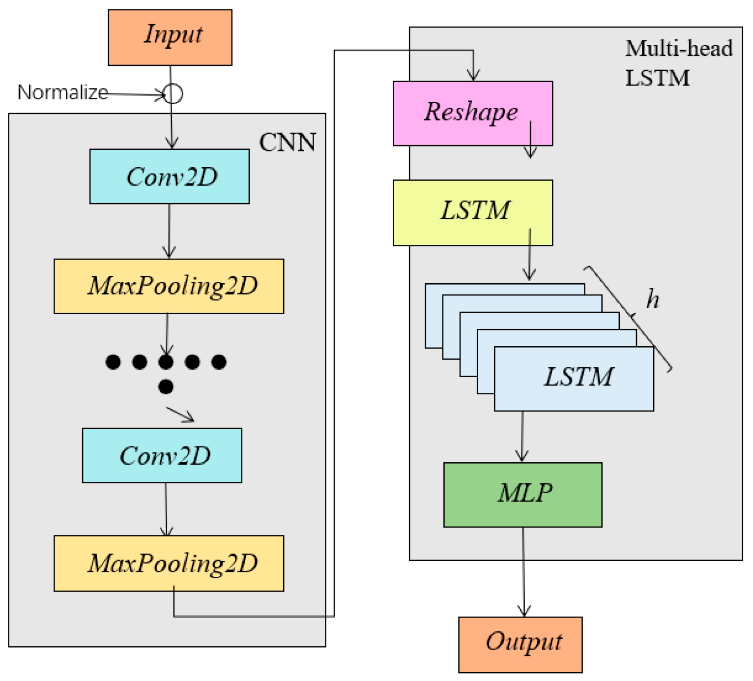
2. CNN-Multi-Head-LSTM Model with an Attention Module Embedded (CMLA)

2.1. Overall Architecture of CMLA

The overall architecture of the CMLA model proposed in this paper is shown in Figure 1.
As shown in Figure 1, after the input data is normalized, the local features of the data are extracted through multiple CNN layers, and the output data of CNN is mapped to a suitable plane and inputted into a multi-head LSTM network. Then, the output is spliced, the distributed features are connected with the tag values through a fully connected neural network (MLP), and, finally, the results are obtained.

2.2. Convolutional Neural Network

Considering the advantages of the CNN in local feature extraction, it is very suitable for processing time series-type fault waveform data [31,32,33]. The input of the model is in time series fault waveform record data at both ends of the line, so one-dimensional convolution neural network is used to extract fault features. Deep data features are extracted through layer-by-layer convolution and pooling operations, as shown in Equations (1) and (2).
h c t = σ c n n W c n n x t + b c n n
where W c n n is the weight coefficient (convolution kernel) of the filter, x t is the t-th input sample, * is the discrete convolution operation,   b c n n is the bias coefficient, σ c n n is the activation function, and h c t is the t-th feature map obtained after performing the convolution.
y t q   = M a x p o o l i n g h c t i  
where h c t i   is the activation value of the i-th neuron in the t-th feature map in the pooling layer and y t q is the output value of the q-th neuron in the t-th feature map.

2.3. Attention Module

In fault location research, the fault features are mainly reflected in the sudden change of electrical quantity, so temporal characteristics in the time dimension are not of the same importance. Compared with the features of the smooth operation period, the features of the sudden change moment are more important. The standard CNN model may ignore the important features; therefore, the attention module is embedded into the CNN network.
The attention mechanism is a calculation that measures the similarity between a query and a key, and performs weighted summation on the values corresponding to the query. It has been widely used in the RNN network. With the deepening of research, a lightweight attention module can be flexibly embedded into the CNN network, which can effectively enhance the feature extraction ability of the CNN at the cost of a small increase in the number of parameters. In this paper, a CBAM module (convolutional block attention module) [34] is introduced into the CNN network to weigh all input features individually, focusing on a specific space and channel, so as to realize the extraction of important features of the recorded data. CBAM constructs a spatial attention module (SAM) and a channel attention module (CAM) to integrate the attention information of the two aspects to obtain more comprehensive feature information. The structure is shown in Figure 2.
For a characteristic F(H×W)the mathematical expression of channel attention is given as follows:
A v g p = M L P [ A v g P ( F ) ] M a x p = M L P [ M a x P ( F ) ] M c ( F ) = σ ( A v g p + M a x p )
where A v g P and M a x P are the average and max pooling, respectively, M L P is the neural network, σ is the activation function, and M c F is the channel attention characteristic matrix (W × 1).
The mathematical expression of spatial attention is given as follows:
M ( F ) = [ A v g P ( F ) , M a x P ( F ) ] M s ( F ) = σ ( f ( M ( F ) ) )
where [] represents the channel stitching operation, f represents the convolution operation, and M s F is the obtained spatial attention characteristic matrix (H × 1).
The calculation equation of the fused characteristic matrix is given as follows:
F = F M
where F is the fused characteristic matrix and represents the multiplication of corresponding elements. CBAM first obtains the channel attention characteristic matrix M c F by passing the characteristic matrix F through SAM, and then obtains the characteristic matrix F after F and M c F . Then, the spatial attention characteristic matrix M s F is obtained through CAM, and the final characteristic matrix F is obtained after the fusion of F and M s F . In this paper, in order to ensure the integrity of recording data input of each channel, the convolution kernel size is set as 1 × 3.
The attention module includes channel attention, spatial attention, and CBAM which combines them. The type, number, and location of attention modules will affect the model. The CNN model in this paper consists of two convolution pooling layers: a single channel and spatial attention, and one or more CBAM modules. Experiments were performed and the results are shown in Appendix A. The experiments show that the single attention module cannot improve the performance of the model as much as the CBAM module, and the effect of one CBAM model is less than that of two CBAM modules. Therefore, CBAM modules are added after each convolution pooling layer to form the CNN-CBAM model.

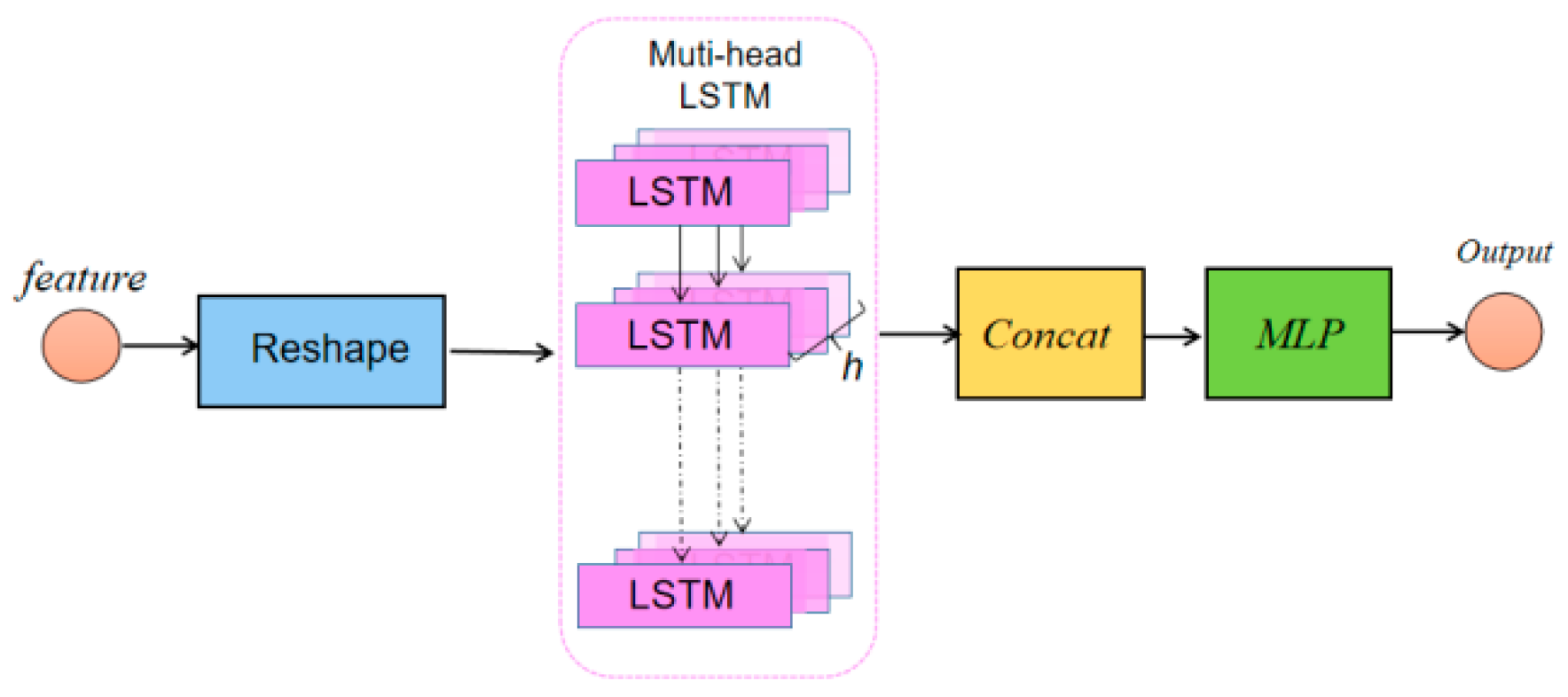
2.4. Multi-Head-LSTM Network

The LSTM model has a built-in forget gate on the basis of the RNN to overcome the gradient vanishing problem. LSTM has two hidden states, h t and S t , and the forget gate determines the probability of forgetting the state of the upper layer of hidden cells.
f t = σ ( W F h ( t 1 ) + U f x t + b f )
In the equation, σ is the sigmoid activation function. The input gate consists of two parts. The first part outputs i t and uses the sigmoid function, while the second part outputs g t and uses the tanh function.
i t = σ ( W i h ( t 1 ) + U i x t + b i )
g t = t a n h ( W a h ( t 1 ) + U a x t + b a )
The status is updated from S t 1 to S t .
S t = S ( t 1 ) f t + i t g t
h t = σ ( W 0 h ( t 1 ) + U 0 x t + b 0 ) t a n h ( S t )
where is the Hadamard product and h t is the output result of the output gate.
In practice, the multi-layer stacked LSTM network can complete more complex prediction tasks, but the serial training structure is prone to the problems of gradient disappearance, over fitting, and a long training time. In order to reduce the depth of the model and improve the network training performance, this paper proposes a multi-head-LSTM network to solve the problem of fault location, and its structure is shown in Figure 3. The improvement idea of multi-head-LSTM comes from the multi-head attention mechanism in the transformer model reported in [35].
In Figure 3, the feature data extracted by the two-layer CNN is reshaped into the input form for the multi-head-LSTM network through one layer of a reshape network. The inputs of all LSTM layers originate from the same data, but the weight matrix values of each layer are different in the process of model training, which strengthens the ability of the model to capture information from different perspectives. In addition, the depth of the model will not increase with the number of LSTM layers, which is equivalent to changing the original multi-layer LSTM network running in series into a multi-head LSTM network running in parallel, which is conducive to accelerating the convergence of the model. The role of the module MLP (multilayer perceptron) is mainly to link the information obtained from model training with the tag value through dimensionality reduction.

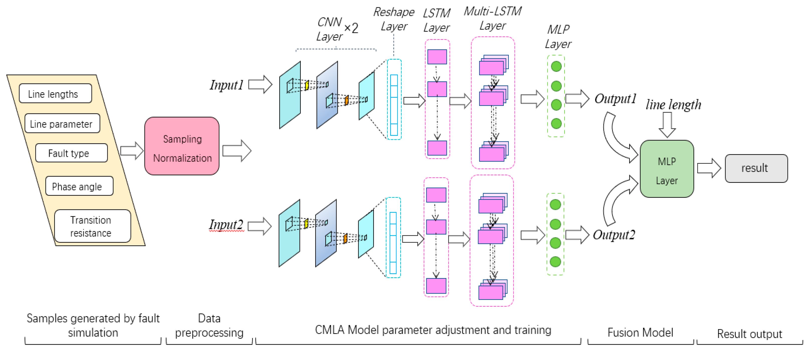
3. Fault Location Based on CMLA Model

3.1. Basic Process

The overall process of fault location of transmission line proposed in this paper is shown in Figure 4.
The time series data of 12 electrical quantities, including three-phase voltage and three-phase current collected by two terminals, are used as the input of the model. These voltage and current timing data, which contain the characteristic information of fault location, are coupled into vectors and form a dimension of 12 × 40 characteristic graphics. Since the dimension of the input data is not too large, there is no need to design a network structure that is too deep. This model is designed as a combination of a two-layer convolution pooling CNN structure, two CBAM attention modules, and a two-layer LSTM structure, one of which is a multi-head-LSTM layer.
Consistent with the input dimension, the CNN model is designed as one-dimensional convolution (Conv1D), the size of the convolution kernel is 1×3, and the number is 64. The maximum pooling (Maxpooling1D) is selected, and the size is 2. After a convolution pooling operation and assessment of the CBAM module, this module does not change the dimension of the input data, but only gives differential weights to specific channels and a feature matrix. After a layer of convolution pooling and attention module, the extracted feature matrix is obtained. TimeDistributed is added to the outer layer of the convolution pooling layer for dimension expansion, and then the Reshape operation is performed to access the LSTM network layer. Finally, by passing through a fully connected layer (MLP), the prediction result of the model is obtained.

3.2. Hyperband Optimization Algorithm

Hyperparameters have a significant impact on the performance of a machine learning model. Based on the tensorflow 2.0 development platform, this paper uses the Hyperband algorithm [36] to optimize the hyperparameters. The Hyperband algorithm is an extension of the Successive Halving algorithm. Compared with Grid Search and Random Search in the early days of machine learning, the Hyperband algorithm is more purposeful. Compared with Bayesian optimization, the Hyperband algorithm has a higher resource utilization efficiency and a faster calculation speed.

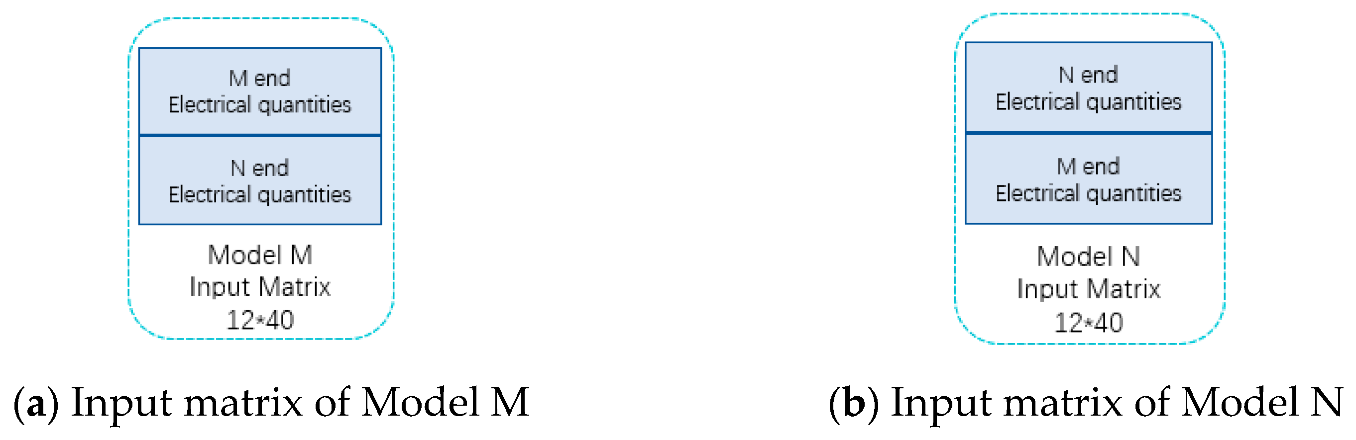
3.3. Fusion CMLA Model with the MLP Output Layer (FCMLA)

It should be noted that this model is supervised learning, and the setting of the label value is related to the observation point. A large number of experimental results show that the fault location accuracy of the model at different observation points (M end, N end) fluctuates in a small range and chases each other, especially for the examples where the line length of the training set is greatly different from that of the test set, and the fault point is biased to one side.
In order to avoid the interaction between long and short lines and fault points, and strengthen the generalization ability of the model to different lines, this paper proposes a fault location method based on the double end fusion model to optimize the original model. If the results of different observation points are fused for training and learning, higher fault location accuracy may be obtained. The basic idea is as follows:
Input1 is the input of Model M, including the electrical quantity data at both ends. The input matrix is the same as that described above, as shown in Figure 5a, and output1 is the output of Model M, and its value is the fault distance relative to the M end. Input2 is the input of Model N, and its data is the same as input1, but the composition of the input matrix has changed, as shown in Figure 5b. In addition, by adding the line length to the input vector, the model can adjust the fault location results according to the line length.
By adding another MLP output layer, the fault location results of the models on both sides are combined, as shown in Figure 5. The MLP output layer adopts the distributed training method. Since Model M has been trained above, only one Model N and one integrated MLP output layer need to be trained. In order to save time and improve the training efficiency of the model, this paper transfers the weight parameter values trained based on Model M to Model N without parameter adjustment. After several iterations, a more satisfactory result can be obtained. The structure of the MLP output layer in this paper is (16,64,8,1), and the sigmoid activation function is adopted.

3.4. Experimental Evaluation Index and Optimization Algorithm

This paper uses three error indicators to evaluate the results, namely the root mean square error ( RMSE), the mean absolute error (MAE), and the mean absolute percentage error (MAPE).
X R M S E = t = 1 N [ x ( t ) x ^ ( t ) ] 2 / ( N 1 )
X MAE = t 1 N x ( t ) x ^ ( t ) / N
X MAPE = 100 % N t 1 N [ x ( t ) x ^ ( t ) ] / x ( t )
where x ( t ) is the actual value of the fault distance, x ^ ( t ) is the model predicted value, and N is the number of test samples.

4. Simulation and Analysis

4.1. Transmission Line Simulation Model Building

According to the commonly used conductor type and length distribution information of 220 kV transmission lines in a certain area of Guangdong Power Grid, a double-ended transmission line model is established with PSCAD/EMTDC. The simplified schematic model is shown in Figure 6, and the line parameters are given in Appendix B. We obtain the training data through different parameter settings of the simulation system, which was set to fail at 0.4 s, with a failure duration of 60 ms and a total simulation time of 0.1 s. Lines 1, 2, and 3 have 1872, 1944, and 2592 sets of fault data, respectively. The total training data size is 6408, and the ratio of training data to validation data is 9:1.

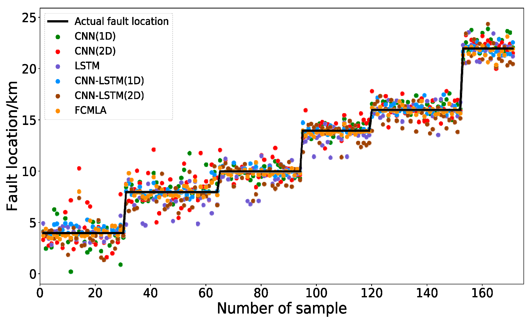
4.2. Location Accuracy Analysis of the Model

In order to verify the effectiveness of the FCLMA model, the CNN model and the LSTM model are used for comparative experiments. The two-layer convolution pooling structure of Conv 1D, Max pooling1D, Conv 2D and Max pooling2D are studied with the CNN model. The size of the convolution kernel is 1 × 3 (1D) and 3 × 3 (2D). The LSTM model adopts the two-layer LSTM, and the number of neurons and super parameters in the model are determined by the Hyperband algorithm.
Table 1 gives the prediction performance analysis of the single model and decomposed combined model. It shows that the FCMLA model has a better performance than the single CNN model and the LSTM model, and the one-dimensional convolution structure of the CNN-LSTM model has a better feature extraction effect than the two-dimensional convolution structure.
The performance of the FCMLA module is more stable and accurate than other models, and its performance on the test set is shown in Figure 7 and Figure 8. In Figure 7, except for the FCMLA, the rest of the models have serious deviations in some data points. CNN (1D) and CNN (2D) show significant deviations (with relatively large location errors) when the fault distance is closer, while LSTM has larger errors when the fault distance is located at the middle of the line, and the combined CNN and LSTM model performs better. In Figure 8, the combined model CNN-LSTM (1D) performs better than CNN-LSTM (2D), which is due to the fact that the input of the model is fault-recorded data, which is different from the images and has a strong temporal correlation, and it is appropriate to use one-dimensional convolution. On the other hand, the FCMLA performs even better, and the samples of the test set are closer to the actual values with less error, indicating that the addition of the attention mechanism can help to obtain more valuable feature data and improve the accuracy of the model.
Compared with previous shallow intelligent algorithms combining data processing methods, such as SVR, KNN, and DT, the performance of different models is shown in Table 2. The data preprocessing may ignore important features, and the nonlinear fitting ability of the shallow model is not as good as the deep model; previously leading shallow intelligent algorithms perform worse. Compared with the SAE model, which also uses feature self-extraction, CNN-CBAM has better feature extraction performance and a higher location accuracy.
In order to verify the effectiveness of the CMLA model, this paper uses the CMLA single model to conduct comparative experiments.
For the mixed data set composed of line 1, line 2, and line 3, the location performance of the CMLA model is shown in Figure 9, and the error is mainly concentrated between +0.5 km and −0.5 km. Table A4 shows that structure and parameters of the CMLA combined model.

4.3. Generalization Performance Analysis of the Model

The trained fusion model from the training sets of lines 1, 2 and 3 is used to derive the fault location of new lines 4 and 5, which are not in the training sets, and the results are shown in Table 3.
It can be seen from the results in Table 3 that the two-terminal fusion CMLA model is able to meet the fault location requirements of various lengths of lines.
The error statistics of a large number of test sets with different fault parameter settings in lines 4 and 5 are shown in Table 4. It can be seen that the fusion FCMLA model has a better fault location performance than the single model, and even though lines 4 and 5 are not in the training set, the fault location accuracy is satisfactory.

4.4. Comparison of Training Speed of Different Depth Models

In this paper, several different deep learning models are built with tensorflow, including CNN1D, CNN2D, CNN2D-LSTM, and Conformer [37] models. By using the same training set, the best performance of each model is compared in the verification set when the number of training rounds is 200. The results are shown in Figure 10. Among them, the training speed of CNN1D is 0.2 s/round, that of CNN2D is 5 s/round, that of CNN2D-LSTM is 11s/round, that of Conformer is 33 s/round, and that of FCMLA is 7 s/round.
From Figure 10, the best performance in 200 rounds of training is given by the Conformer and FCMLA model, but from the perspective of training time, the CMLA model is significantly better than the Conformer. Compared with the traditional multi-layer CNN-LSTM model, the FCMLA model not only has fast training speed, but also has superior performance. The main reason is that the LSTM layer in CNN-LSTM is connected in series, and the parameters of the previous layer need to be calculated before proceeding to the next layer. The LSTM layers in the FCMLA model are connected in parallel, and multiple LSTM layers can be trained simultaneously, thus reducing the depth of the model and increasing the width, which is conducive to improving the training speed. Moreover, the parameters learned by each LSTM layer are different, so as to collect the characteristics of the data set in a larger range and improve the performance of the model.

5. Conclusions

Aiming at addressing the issues that traditional intelligent fault location algorithms require a manual design of complex feature extraction methods and line-specific modeling, as well as the generalization performance not being high, this paper proposes a fusion model based on CNN-multi-head-LSTM with an attention module to realize power transmission line fault location, through theoretical analysis and experimental verification, the following conclusions are obtained.
(1)
Compared with the artificially designed feature extraction method, the proposed FCMLA model (fusion CNN-multi-head-LSTM with an attention module) obtains more important feature distributions through selective feature self-learning, which is beneficial to the subsequent LSTM to capture the timing characteristics and achieve accurate fault location.
(2)
The multi-head LSTM model based on the “multi-head” idea not only obtains a higher fault location accuracy, but also improves the training speed of the multi-layer depth model. The reason is that the original multi-layer series LSTM layer is transformed into a parallel connection, so as to realize the synchronous training and comprehensive feature extraction of multiple LSTM networks.
(3)
Due to the difference in the fault location accuracy of the model when the fault point is close to different sides, the stability of the final fault location result is improved by adding a full connection layer to fuse the results of the models on both sides.
(4)
The final fault location results of the FCMLA model proposed in this paper can meet the needs of practical applications. The simulation results show that its generalization ability can adapt to the differences of line length and parameters.

Author Contributions

Q.Y. and L.L.L. guided the framework of the paper and provided professional guidance. C.S. and X.W. performed the simulation and wrote the paper. C.S.L. provided academic assistance and revised the manuscript. All authors have read and agreed to the published version of the manuscript.

Funding

This work was supported by the National Natural Science Foundation of China [Project Number 52177119].

Informed Consent Statement

Not applicable.

Conflicts of Interest

The authors declare no conflict of interest.

Appendix A

Table A1. Performance of the model with different positions of the attention module.
Type of Attention ModuleLocationEvaluation Indicators
RMSEMAEMAPE
CAMMaxpooling10.7760.5446.4%
SAMMaxpooling10.7200.47644.6%
CBAMMaxpooling10.75820.47455.34%
CBAMMaxpooling20.58360.40473.99%
CBAMMaxpooling1,20.54180.37144.60%
Table A2. Parameters of different lines.
Parameter TypeZero-Sequence
Parameter
Positive-Sequence
Parameter
Line
R/(Ω/km)0.228460.01979Line 1
L/(mH/km)2.772380.87579
C/(uF/km)8.5809 × 10−313.310 × 10⁻³
R/(Ω/km)0.30.03648Line 2
L/(mH/km)3.6391.348
C/(uF/km)6.166 × 10−38.68 × 10−3
R/(Ω/km)0.11480.02083Line 3
L/(mH/km)2.288580.8984
C/(uF/km)5.2809 × 10−312.910 × 10⁻³
R/(Ω/km)0.30890.023Line 4
L/(mH/km)2.58740.9372
C/(uF/km)6.3502 × 10−313.71 × 10⁻³
R/(Ω/km)0.36740.054Line 5
L/(mH/km)3.3231.086
C/(uF/km)5.019 × 10−311.068 × 10⁻³
Table A3. Fault settings for different lines.
Parameter TypeParameter SettingNumber of ParametersLine
Voltage level220 kV1Line 1
Fault typeLG, LLG, LLL3
Line length (km)25, 20, 153
Phase angle difference (degree)5, 30, 603
Fault distance (km)L0 = 2,3(initial) Step length = 226
Transition resistance (Ω)0.01, 10, 20, 50, 80, 100, 120, 1508
Voltage level220 kV1Line 2
Fault typeLG, LLG, LLL3
Line length (km)60, 55, 503
Phase angle difference (degree)5, 30, 603
Fault distance (km)L0 = 5,6,8(initial) Step length = 3,436
Transition resistance (Ω)0.01, 10, 20, 50, 80, 100, 120, 1508
Voltage level220 kV1Line 3
Fault typeLG, LLG, LLL3
Line length (km)45, 35, 303
Phase angle difference (degree)5, 30, 603
Fault distance (km)L0 = 3.5,4(initial) Step length = 3,427
Transition resistance (Ω)0.01, 10, 20, 50, 80, 100, 120, 1508
Voltage level220 kV1Line 4
Fault typeLG, LLG, LLL3
Line length (km)301
Phase angle difference (degree)5, 30, 603
Transition resistance (Ω)0.01, 10, 20, 50, 80, 100, 120, 1508
Voltage level220 kV1Line 5
Fault typeLG, LLG, LLL3
Line length (km)701
Phase angle difference (degree)5, 30, 603
Transition resistance (Ω)0.01, 10, 20, 50, 80, 100, 120, 1508

Appendix B

Table A4. Structure and parameters of the CMLA combined model.
Input (12 × 40) M Input (12 × 40) N
Time Distributed (Conv1D (64,3))Time Distributed (Conv1D (256,3))
Time Distributed (Maxpooling (2))Time Distributed (Maxpooling (2))
CBAMCBAM
Time Distributed (Conv1D (32,3))Time Distributed (Conv1D (64,3))
Time Distributed (Maxpooling (2))Time Distributed (Maxpooling (2))
CBAMCBAM
Time Distributed (Flatten ())Time Distributed (Flatten ())
LSTM (64)LSTM (100)
Dense (1)Dense (1)
Output

References

  1. Saha, M.M.; Izykowski, J.J.; Rosolowski, E. Fault Location on Power Networks; Springer Science & Business Media: Berlin/Heidelberg, Germany, 2009. [Google Scholar]
  2. Panahi, H.; Zamani, R.; Sanaye-Pasand, M.; Mehrjerdi, A.H. Advances in transmission network fault location in modern power systems: Review, outlook and future works. IEEE Access 2021, 9, 158599–158615. [Google Scholar] [CrossRef]
  3. Johns, A.T.; Lai, L.L.; El-Hami, M.; Daruvala, D.J. New approach to directional fault location for overhead power distribution feeders. IEE Proc.–Gener. Transm. Distrib. 1991, 138, 351–357. [Google Scholar] [CrossRef]
  4. El-Hami, M.; Lai, L.L.; Daruvala, D.J.; Johns, A.T. A new travelling-wave based scheme for fault detection on overhead power distribution feeders. IEEE Trans. Power Deliv. 1992, 7, 1825–1833. [Google Scholar] [CrossRef]
  5. Tong, N.; Tang, Z.; Lai, C.S.; Li, X.; Vaccaro, A.; Lai, L.L. A novel acceleration criterion for remote-end grounding-fault in MMC-MTDC under communication anomalies. Int. J. Electr. Power Energy Syst. 2022, 141, 108131. [Google Scholar] [CrossRef]
  6. Zhang, C.; Song, G.; Yang, L.M.; Sun, Z. Time-domain single-ended fault location method no need for remote-end system information. IET Gener. Transm. Distrib. 2019, 14, 284–293. [Google Scholar] [CrossRef]
  7. Tong, N.; Tang, Z.; Wang, Y.; Lai, C.S.; Lai, L.L. Semi AI-based protection element for MMC-MTDC using local-measurements. Int. J. Electr. Power Energy Syst. 2022, 142, 108310. [Google Scholar] [CrossRef]
  8. Yu, C.S.; Chang, L.R.; Cho, J.R. New fault impedance computations for unsynchronized two-terminal fault-location computations. IEEE Trans. Power Deliv. 2011, 26, 2879–2881. [Google Scholar] [CrossRef]
  9. Chen, R.; Yin, X.; Li, Y. Fault location method for transmission grids based on time difference of arrival of wide area travelling wave. J. Eng. 2018, 2019, 3202–3208. [Google Scholar] [CrossRef]
  10. Silva, A.; Lima, A.; Souza, S.M. Fault location on transmission lines using complex-domain neural networks. Int. J. Electr. Power Energy Syst. 2012, 43, 720–727. [Google Scholar] [CrossRef]
  11. Farshad, M.; Sadeh, J. Accurate Single-Phase Fault-Location Method for Transmission Lines Based on K-Nearest Neighbor Algorithm Using One-End Voltage. IEEE Trans. Power Deliv. 2012, 27, 2360–2367. [Google Scholar] [CrossRef]
  12. Joorabian, M.; Asl, S.; Aggarwal, R.K. Accurate fault locator for EHV transmission lines based on radial basis function neural networks. Electr. Power Syst. Res. 2004, 71, 195–202. [Google Scholar] [CrossRef]
  13. Silva, K.M.; Souza, B.A.; Brito, N. Fault detection and classification in transmission lines based on wavelet transform and ANN. IEEE Trans. Power Deliv. 2006, 21, 2058–2063. [Google Scholar] [CrossRef]
  14. Samantaray, S.R.; Dash, P.K.; Panda, G. Distance relaying for transmission line using support vector machine and radial basis function neural network. Int. J. Electr. Power Energy Syst. 2007, 29, 551–556. [Google Scholar] [CrossRef]
  15. Jamil, M.; Kalam, A.; Ansari, A.; Rizwan, M. Generalized neural network and wavelet transform based approach for fault location estimation of a transmission line. Appl. Soft Comput. 2014, 19, 322–332. [Google Scholar] [CrossRef]
  16. Hao, Y.Q.; Wang, Q.; Li, Y.N.; Song, W.F. An intelligent algorithm for fault location on VSC-HVDC system. Int. J. Electr. Power Energy Syst. 2018, 94, 116–123. [Google Scholar] [CrossRef]
  17. Tse, N.; Chan, J.; Liu, R.; Lai, L.L. Hybrid wavelet and Hilbert transform with frequency shifting decomposition for power quality analysis. IEEE Trans. Instrum. Meas. 2012, 61, 3225–3233. [Google Scholar] [CrossRef]
  18. Farshad, M.; Sadeh, J. Transmission line fault location using hybrid wavelet-Prony method and relief algorithm. Int. J. Electr. Power Energy Syst. 2014, 61, 127–136. [Google Scholar] [CrossRef]
  19. Ravesh, N.R.; Ramezani, N.; Ahmadi, I.; Nouri, H. A hybrid artificial neural network and wavelet packet transform approach for fault location in hybrid transmission lines. Electr. Power Syst. Res. 2022, 204, 107721. [Google Scholar] [CrossRef]
  20. Liu, C.C.; Stefanov, A.; Hong, J. Artificial Intelligence and Computational Intelligence: A Challenge for Power System Engineers; John Wiley & Sons, Inc.: Hoboken, NJ, USA, 2016. [Google Scholar]
  21. Luo, G.M.; Hei, J.X.; Liu, Y.Y.; Li, M.; He, J.H. Fault location in VSC-HVDC using stacked denoising autoencoder. In Proceedings of the 2019 IEEE 3rd International Electrical and Energy Conference (CIEEC), Beijing, China, 7–9 September 2019; pp. 36–41. [Google Scholar]
  22. Li, X.T.; Qin, L.W.; Li, Y.Z.; Yang, X.; Yu, X.Y. Fault location of distribution network based on stacked autoencoder. In Proceedings of the 16th Annual Conference of China Electrotechnical Society, Singapore, 24–26 September 2022; pp. 564–572. [Google Scholar]
  23. Luo, G.; Yao, C.; Liu, Y.; Tan, Y.; He, J.; Wang, K. Stacked Auto-Encoder Based Fault Location in VSC-HVDC. IEEE Access 2018, 6, 33216–33224. [Google Scholar] [CrossRef]
  24. Zhu, B.E.; Wang, H.Z.; Shi, S.X.; Dong, X.Z. Fault location in AC transmission lines with back-to-back MMC-HVDC using ConvNets. J. Eng. 2019, 2019, 2430–2434. [Google Scholar] [CrossRef]
  25. Lan, S.; Chen, M.; Chen, D.Y. A novel HVDC double-terminal non-synchronous fault location method based on convolutional neural network. IEEE Trans. Power Deliv. 2019, 34, 848–857. [Google Scholar] [CrossRef]
  26. Shadi, M.R.; Mohammad-Taghi, A.; Sasan, A. A real-time hierarchical framework for fault detection, classification, and location in power systems using PMUs data and deep learning. Int. J. Electr. Power Energy Syst. 2022, 134, 107399. [Google Scholar] [CrossRef]
  27. Hei, J.; Luo, G.; Cheng, M.; Liu, Y.; Tan, Y.; Li, M. A research review on application of artificial intelligence in power system fault analysis and location. Proc. CSEE 2020, 40, 5506–5516. [Google Scholar]
  28. Duan, Y.; Yuan, H.L.; Lai, C.S.; Lai, L.L. Fusing local and global information for one-step multi-view subspace clustering. Appl. Sci. 2022, 12, 10. [Google Scholar] [CrossRef]
  29. Chen, R.; Lai, C.S.; Zhong, C.; Pan, K.; Ng, W.W.Y.; Li, Z.L.; Lai, L.L. MultiCycleNet: Multiple cycles self-boosted neural network for short-term household load forecasting. Sustain. Cities Soc. 2022, 76, 103484. [Google Scholar] [CrossRef]
  30. Lai, C.S.; Yang, Y.; Pan, K.; Zhang, J.; Yuan, H.; Ng, W.W.Y.; Gao, Y.; Zhao, Z.; Wang, T.; Shahidehpour, M.; et al. Multi-view neural network ensemble for short and mid-term load forecasting. IEEE Trans. Power Syst. 2021, 36, 2992–3003. [Google Scholar] [CrossRef]
  31. Gretton, A.; Borgwardt, K.M.; Rasch, M.J.; Scholkopf, B.; Smola, A. A kernel two-sample test. J. Mach. Learn. Res. 2012, 13, 723–773. [Google Scholar]
  32. Jia, R.; Song, Y.C.; Piao, D.M.; Kim, K.; Lee, C.Y.; Park, J. Exploration of deep learning models for real-time monitoring of state and performance of anaerobic digestion with online sensors. Bioresour. Technol. 2022, 363, 127908. [Google Scholar] [CrossRef]
  33. Liang, J.; Jing, T.; Niu, H.; Wang, J. Two-Terminal Fault Location Method of Distribution Network Based on Adaptive Convolution Neural Network. IEEE Access 2020, 8, 54035–54043. [Google Scholar] [CrossRef]
  34. Woo, S.; Park, J.; Lee, J.Y.; Kweon, I.S. Cbam: Convolutional block attention module. In Proceedings of the European Conference on Computer Vision (ECCV), Munich, Germany, 8–14 September 2018; pp. 3–19. [Google Scholar]
  35. Vaswani, A.; Shazeer, N.; Parmar, N.; Uszkoreit, J.; Jones, L.; Gomze, A.N.; Kaiser, L.; Polosukhin, I. Attention is all you need. arXiv 2017. [Google Scholar] [CrossRef]
  36. Li, L.; Jamieson, K.; DeSalvo, G.; Rostamizadeh, A.; Talwalkar, A. Hyperband: A novel bandit-based approach to hyperparameter optimization. J. Mach. Learn. Res. 2017, 18, 6765–6816. [Google Scholar]
  37. Peng, Z.; Huang, W.; Gu, S.; Xie, L.; Wang, Y.; Jiao, J.; Ye, Q. Conformer: Local Features Coupling Global Representations for Visual Recognition. IEEE Int. Conf. Comput. Vis. 2021, 357–366. [Google Scholar] [CrossRef]
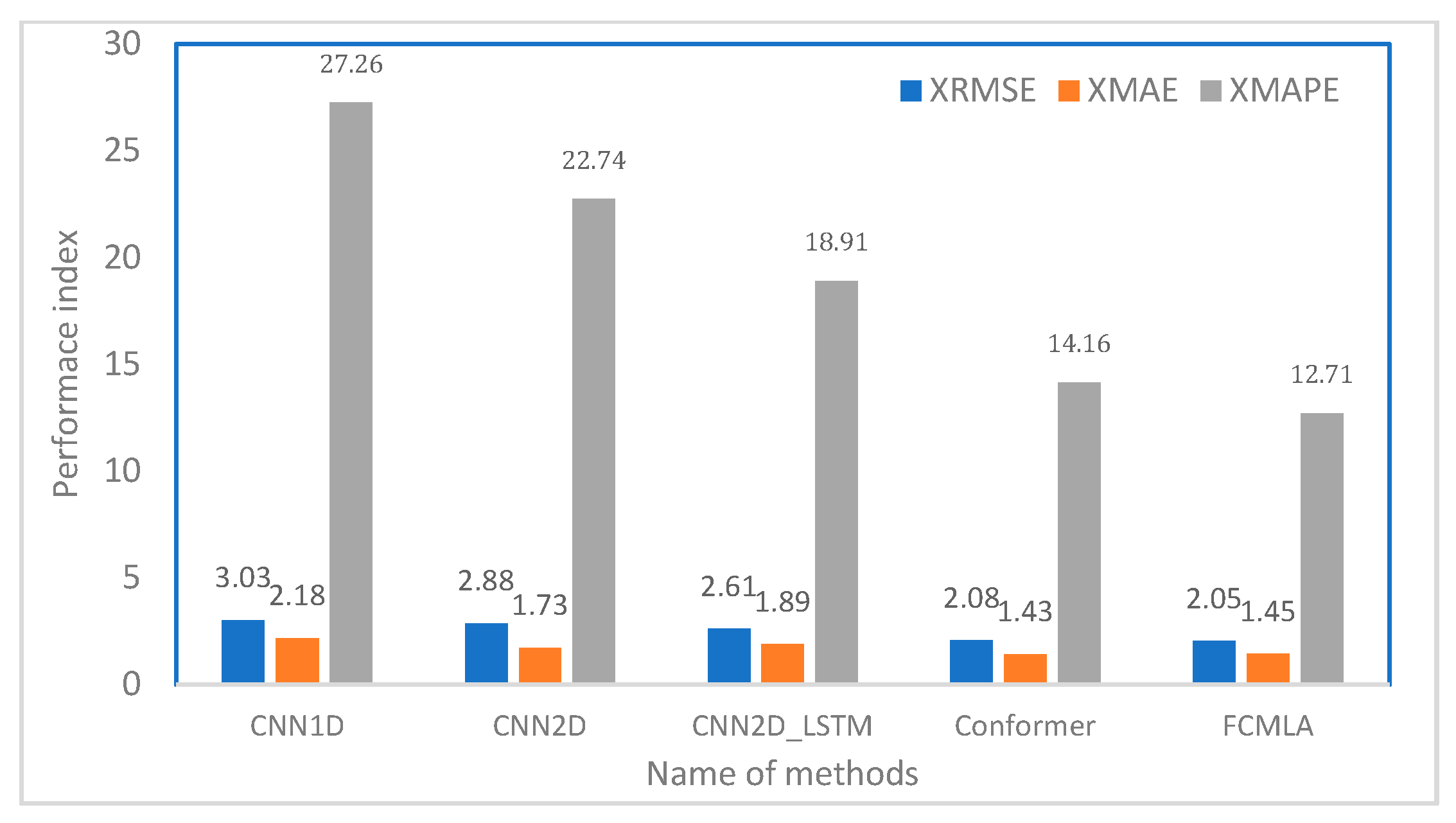
Figure 1. Structure of the CMLA model.
Energies 16 01827 g001
Figure 2. Structure of the CBAM.
Energies 16 01827 g002
Figure 3. Structure of the multi-head-LSTM.
Energies 16 01827 g003
Figure 4. Architecture of the fault location.
Energies 16 01827 g004
Figure 5. Input matrix of Model M and Model N.
Energies 16 01827 g005
Figure 6. Simplified simulation diagram of the transmission system.
Energies 16 01827 g006
Figure 7. Predicted and real values for different decomposition models.
Energies 16 01827 g007
Figure 8. Distribution of location results from No. 95 to No. 120.
Energies 16 01827 g008
Figure 9. Error of test data set.
Energies 16 01827 g009
Figure 10. Performance comparison of each model training for 200 rounds.
Energies 16 01827 g010
Table 1. Fault location performance of different models.
Predictive ModelXRMSEX MAEX MAPE
CNN (1D)0.84600.65218.22%
CNN (2D)1.17600.866510.87%
LSTM1.09160.78408.53%
CNN-LSTM (1D)0.57730.53233.99%
CNN-LSTM (2D)1.08290.84619.62%
FCMLA0.54180.37144.60%
Table 2. Fault location performance of different models.
Predictive ModelXRMSEX MAEX MAPE
KNN2.7291.76816.43%
SVR1.4140.9577.20%
DT0.6630.2183.31%
WT-DT1.4310.3772.09%
FFT-DT1.4700.4612.62%
SAE0.8860.4213.4%
CLMA0.54180.37144.60%
Table 3. Fault location performance of different models.
LineLength (km)Fault Location
(km)
Average Fault Location Result (km)
Forecast ResultError
4301514.5120.488
5704040.765−0.765
Table 4. Fault location performance of different models.
Predictive ModelXRMSEX MAEX MAPE
CMLA (single)-M0.54180.37144.60%
CMLA (single)-N0.55130.40233.60%
FCMLA (fusion MCLA)0.46250.30420.84%
Disclaimer/Publisher’s Note: The statements, opinions and data contained in all publications are solely those of the individual author(s) and contributor(s) and not of MDPI and/or the editor(s). MDPI and/or the editor(s) disclaim responsibility for any injury to people or property resulting from any ideas, methods, instructions or products referred to in the content.

