Abstract
The continuous increase in generation from renewable energy sources, marked by correlated forecast uncertainties, requires specific methodologies to support power system operators in security management. This paper proposes a probabilistic preventive control to ensure N-1 security in presence of correlated uncertainties of renewable sources and loads. By adopting a decoupled linear formulation of the AC load flow equations, the preventive control is decomposed into two subsequent linear programming problems, the former concerning the active power and the latter the voltage/reactive power-related issues. In particular, in the active control problem, the algorithm combines Third Order Polynomial Normal Transformation, Point Estimate Method, and Cornish–Fisher expansion to model the forecast uncertainties and characterize the chance constraints in the problem. The goal is to find the optimal phase shifting transformer tap setting, conventional generation redispatching, and renewable curtailment at the minimum cost to assure the probabilistic fulfillment of N and N-1 security constraints on branch active power flows. The second stage solves another linear programming problem, which aims to minimize the adjustments to generators’ set-point voltages to avoid violations at node voltages and branch-rated limits due to reactive power flows while meeting generator reactive power constraints. Simulations performed on an IEEE test system demonstrate the effectiveness of the proposed security control method in limiting the probability of violating security limits in N and N-1 state, including voltage/reactive power constraints, in presence of correlated uncertainties.
1. Introduction
The spread of Renewable Energy Sources (RES) is profoundly changing the planning and operation of power systems. In general terms, the large-scale integration of renewables has brought a higher level of uncertainty in the electric system due to their stochastic and intermittent generation.
For this reason, the uncertainty management represents a fundamental step for the efficient and economical operation of electric systems. Therefore, specific strategies for uncertainty management are crucial to favor RES penetration and guarantee the grid’s security.
Different sources of uncertainty have to be considered according to the phase of power system management, from long term planning to operational planning and quasi-real-time control [,]. In an operational planning context, important sources of uncertainty regard the load demand and renewable generation forecast, as well as the outages of components, also accounting for incumbent adverse weather conditions. On the other hand, neglecting forecast uncertainties in power system management may lead to security issues [,].
Therefore, advanced methods are needed to address uncertainties to minimize the probability of violating system operational limits.
In this context, probabilistic methodologies based on Chance Constrained (CC) formulation [,,,,,], wherein the constraints are formulated in terms of violation probability of operational limits, can be very useful. Authors in [] analyze different mathematical formulations of the chance constraints that, however, cannot consider specific properties (e.g., asymmetry) of the probabilistic distributions and their correlations. Reference [] proposes the CC and Security Constrained Optimal Power Flow (SC-OPF), exploiting corrective actions from control devices like Phase Shifting Transformers (PSTs) and HVDC links. In [], a CC OPF formulated as a convex conic optimization problem is presented together with an efficient cutting plane algorithm for its solution. Authors in [] describe a real-time CC dispatch based on quadratic programming and dynamic power flow. This approach also considers constraints on conventional generator ramps on frequency deviation. In addition, the chance constraints are modeled through Cornish–Fisher expansion and cumulants’ methodology. The solution proposed in [] incorporates generator reserve within the CC formulation. Authors in [] propose an SC OPF based on CC that explicitly considers the probability of contingency events and potential failures in the operation of post-contingency corrective controls. It can be remarked this work is based on a full AC model solved through a heuristic approach but it does not consider uncertainties on load and RES injections. In [], an algorithm for solving joint CC DC OPF problem is proposed, using a sample-based approach that avoids making strong assumptions on the distribution of the uncertainties and scales favorably to large problems. In [], quadratic programming for the AC OPF is proposed for applications in smart distribution networks. This approach exploits linear constraints to represent power losses, resulting in a trade-off between accuracy, performance, and robustness. Finally, [] presents a risk-based CC optimal power flow model by leveraging the methods of both adjustable uncertainty set and robust optimization.
The present paper proposes an innovative CC and SC control that assures the probabilistic fulfillment of N-1 security constraints in presence of forecast uncertainties due to renewable sources and loads. To this aim, it performs a set of preventive actions, i.e., the redispatch of active powers injected by conventional generators, the regulation of Phase Shift Transformers, and the renewables’ curtailment, to solve active power-related issues. However, it can also adjust the voltage references of the generating units to solve potential issues related to voltages and reactive powers.
The proposed methodology uses Point Estimate Method (PEM) and Third order Polynomial Normal Transformation (TPNT) [,] to obtain the raw moments (and, therefore, the cumulants) of the quantities subject to constraints (e.g., active power flows), taking into account correlated forecast uncertainties.
The control is formulated as a two-stage problem: the former stage is formulated as a linear programming problem, including a linearized model for PSTs based on distribution factors, with the final aim to minimize the redispatching cost of conventional generators and renewable curtailment. The chance constraints concern the technical limits of generators, the invariance of total generation (conventional and from RES), and the active power flow limits both in state N and N-1. The chance constraints are formulated as inequalities that involve quantiles of uncertain variables evaluated from cumulants through the Cornish–Fisher expansion. The first stage represents an upgrade of the work presented in [], integrating a linearized model of the PSTs for active power flow management. The latter stage is additional with respect to [], and it is formulated as a linear programming problem on a linearization of the original AC power flow equations. In this stage, the control variables are the variations of voltage reference set-points at PV generation buses, with the aim to avoid violations at PQ node voltages and at branch rated limits, limiting the relevant reactive power flows while meeting the generator reactive capability limits.
It is essential to highlight that the proposed two-stage approach has been designed consisting of two linear optimization algorithms for its future application to large electrical networks, thus, limiting the computational burden and guaranteeing globally optimal solutions. Finally, the presented methodology has been implemented in Matlab/GAMS environment, exploiting GAMS [] as specific software for optimization problems improving the implementation and the computation efficiency with respect to the architecture used in [] completely relying on Matlab.
In summary, this paper provides the following contributions:
- The proposal of a two-stage formulation of the control as an efficient linear programming problem, which includes both active power-related and voltage/reactive power-related constraints. The latter ones are not considered by all the works reported in the introduction, except for [], which proposes a heuristic solution of the full AC power flow.
- The integration of a linearized model of the AC power flow equations favors the decoupling of active and reactive power control problems in the proposed security-constrained preventive control strategy.
- The design and the implementation of a linear optimization algorithm for the Volt/Var control (i.e., the second stage of the proposed CC and SC control) which is based on the above-mentioned linearized model and which receives the inputs from the active power control stage.
- The integration of a linearized model of the PSTs, based on Phase Shifter Distribution Factors (PSDFs), for the active power flow management within the first stage of the presented methodology. The adoption of PSDF-based modeling for PSTs, together with the linearization of AC power flow equations, allows one to maintain a linear programming formulation that can be solved in a very efficient way.
The paper is organized as follows: Section 2 presents the preliminary requirements in terms of power system modeling for the definition of the proposed control framework and Section 3 describes the detailed mathematical formulation. Section 4 presents the case study and the simulation scenarios and describes the results obtained from the application of the algorithm. Section 5 concludes.
2. Power System Modeling: Preliminary Requirements for an Effective Integration into the Control Framework
Before formulating the proposed control, it is important to describe the techniques available from the literature briefly and used in the present approach to effectively integrate some aspects of power system operation in the control framework. This integration has been implemented to preserve a linear formulation which is very time efficient. Specifically, the control will benefit from:
- The linearization of AC power flow equations, based on the technique in [].
- The representation of control devices, specifically the Phase Shifting Transformers (PST), based on the application of PSDFs [,].
- The representation of the asymmetric distributions and the correlation of forecast uncertainties for RES generation and load absorption in the chance constraints of the control, combining the following techniques, namely the Third Order Polynomial Normal Transformation, the Point Estimate method [,], and the Cornish–Fisher expansion [].
In the sequel, these techniques are recalled with the relevant references.
2.1. AC Power Flow Linearization
This subsection recalls the well-known decoupled linear formulation of the AC power flow in [], defining the quantities and symbols used in the control framework.
To facilitate the paper comprehension, it is helpful to recap the standard equation related to the AC power flow:
where is the active power at node i, is the number of nodes, is the voltage magnitude at node i, is the real part of the element of the admittance matrix, is the imaginary part of the element of the admittance matrix, is the angle difference between node i and k, is the reactive power injection at node i, is the active power flow related to line , is the reactive power flow through line , is the transformer tap ratio of line , while is the half of susceptance of line .
2.1.1. Active Power
In this work, the active power flows and the angles are evaluated with the following assumptions:
Exploiting Equations (5) and (6), Equation (1) becomes:
where is the reactance of line . Equation (7) can be represented also in matrix form as
wherein is the vector of the angles at the buses with entries , while
in which the slack busbar row and column are deleted. Inverting gives
Similarly, using Equations (5) and (6), Equation (3) can be written as
from which substituting Equation (10) gives
in which if bus i is slack, , and therefore:
Notice that for the active power, this decoupled approach is equivalent to the DC power flow [].
2.1.2. Reactive Power
As far as reactive power is concerned, in this formulation, the linearization is performed starting from the assumption that the voltage magnitudes are close to 1 p.u.
Notice that , with and calculated through Equation (10).
At this point, it is possible to write Equation (17) in matrix form as
and also its partition in blocks:
where is the vector of PQ nodes while is the vector of PV nodes and slack bus.
From Equation (21), the following relations can be obtained:
where is the number of PQ nodes, is the number of PV nodes plus slack bus, and
Finally, exploiting the assumption that the voltage magnitudes are close to 1 p.u within Equation (4), it is possible to write the reactive power flows as
where
2.2. PST Modeling
The technique exploited in this work is taken from [,] and is based on the phase shifter distribution factors that are similar to the Power Transfer Distribution Factors (PTDF) [], which will be used in the proposed formulation to evaluate the contribution on the active power control.
The PST has proven to be a robust technology that can significantly contribute to regulating power flows [,,].
The implemented model of the PST is approximate, but according to [,], the accuracy is very satisfactory as long as the PST angle is not extremely large (>30°).
For the sake of clarity, this subsection briefly recalls the well-known formulation of the PSDFs, defining the quantities and symbols used in the control framework. In particular, the notation is the same in Section 2.1. If a single PST with a phase shift is located in series with a line , the active power through that line can be evaluated as [,]:
where is the value of the flow with (i.e., without PST), while is the PSDF calculated as
where terms are computed according to Equation (9).
It is worth noting that the presence of a single PST influences the flow of the entire network. Thus, the active power flow of a line without a PST can be evaluated as
where again is the value of the flow with , while is calculated as
2.3. Uncertainty Modeling
The assessment of the probability distributions for the operating quantities (e.g., branch power flows) is performed starting from correlated and non-Gaussian forecast errors by applying a combination of Point Estimation Method and Third Order Polynomial Normal Transformation [].
The former calculates the raw moments of the outputs of a generic function which is fed with m stochastic inputs with known probability distributions by evaluating the aforementioned function in specific tuples of the m variables. The latter technique expresses correlated stochastic variables with non-symmetric probability distributions as combinations of normal independent variables.
The quantiles of the probability distributions related to the operating quantities used in the chance constraints of the control are calculated based on the Cornish–Fisher expansion, which computes the quantile of a distribution starting from the statistical moments of the same distribution. In particular, the quantile for a stochastic variable with skewness S and kurtosis K is given in Equation (37).
where is the quantile of the normal distribution with inverse CDF . More details on these techniques can be found in [].
3. The Proposed Chance Constrained Control: Mathematical Formulation
The present section describes the probabilistic control in presence of forecast uncertainties. By adopting the decoupled linear formulation of the AC load flow equations illustrated in Section 2.1, the preventive control is decomposed into two subsequent linear programming problems, respectively, related to active power and to voltage/reactive power-related issues. Section 3.1 describes the mathematical formulation of the optimization algorithm for active power control, while Section 3.2 describes the mathematical formulation of the optimization algorithm for the Volt/Var control.
3.1. Active Power Control
The algorithm related to the active power control is represented by a security-constrained preventive redispatching of active power conventional generation, including also renewable curtailment and PST control. Furthermore, this active power control can consider the forecast uncertainties on renewable energy sources and load through the definition of a stochastic optimization algorithm based on a Chance Constrained (CC) formulation, wherein the constraints can be formulated in terms of the probability of violating operational limits.
The goal of the proposed redispatching problem is to define a power flow optimization model to minimize the redispatching costs and assure the fulfillment of probabilistic N and N-1 security constraint power flows, taking into account controlled uncertainties in renewable generation and load demand. Thus, the active control algorithm is formulated as a linear programming problem that aims to minimize the redispatching costs related to conventional generation and renewable curtailment.
The proposed optimization procedure exploits the linear approximation of AC power flow equations, described in Section 2.1.
The chance constraints concern the technical limit of the generating unit, the invariance of the global generation (composed of conventional and renewable), and active power flow limits in N and N-1 states. The chance constraints are represented by inequalities involving quantiles of uncertain quantities obtained by Cornish–Fisher expansion from cumulants.
The method presented in this section is an evolution of the one presented in [], including the model of the PSTs in the active power flow management (see Section 2.2 for the PST representation).
The following subsections illustrate the parameters, the variables, and the formulation of the problem (including the reformulation of the chance constraints).
3.1.1. Problem Parameters
This section describes all the parameters for the active power control algorithm.
The considered transmission network is supposed to be composed of: buses, branches, Dispatchable Generation Units (DGUs), Renewable Energy Sources Units (RESUs), PSTs, and loads.
The data supposed to be available are:
- Network buses, branches, and topology parameters. In particular:
- −
- a PTDF matrix, defined in N state, with respect to DGUs, indicated as S (with entries , ) and, with respect to RESUs, indicated as (with entries , ), while with respect to load absorption, indicated as (with entries , ).
- −
- PTDF matrices computed in N-1 conditions, i.e., in presence of contingencies; specifically a set of is considered, and the corresponding PDTF matrices are indicated with , and , with . Notice that the notation used for the entries of these parameters is the same used for the previous point of this list.
- −
- The branches active power rates, indicated as with .
- PST Parameters:
- −
- PSDF matrix in N state indicated as F (with entries , ).
- −
- PSDF matrices in N-1 conditions computed in presence of a line contingency, represented by (with entries , , ).
- Maximum and minimum dispatchable power of DGUs: given the j-th DGU, with , the minimum and maximum level of dispatchable power are indicated with and , respectively.
- Maximum power potentially generated by each RESU: the maximum active power that the h-th RESU can generate, with , is indicated with .
- Initial power dispatch of each DGU, indicated with ().
- Maximum and minimum phase shift for the PSTs: given the y-th PST, the minimum and the maximum angle are indicated with and , respectively.
- Forecasts of the power generated by RESUs: given the h-th RESU, with , the forecast of the generated power indicated with . Moreover, forecasts errors are modeled by a non-symmetric distribution with known moments up to the 4-th moment.
- Forecasts of the power demanded by the d-th load, with , indicated with . Moreover, forecasts errors are modeled by a Gaussian distribution with a known standard deviation.
- Initial power flow: given the initial power dispatch and the forecasts of load demand and RES generation, an initial active power flow is defined as for the -th branch, with .
- Initial power flow under contingency: given the k-th N-1 contingency, with , an initial active power flow is defined as for the -th branch, with .
- Costs of upward and downward generation of DGUs: the upward and downward costs of the j-th DGUs are indicated with and (), respectively.
- Costs of RES curtailment: cost of curtailment of the h-th RESU is indicated with ().
3.1.2. Problem Variables
The optimization variables for the active power control are:
- Upward and downward power set-point variations of the j-th DGU, indicated with and , respectively. These variables are supposed to be positive ().
- Curtailment of the h-th RESU, indicated with . Moreover, this variable is supposed to be positive ().
- Active power flow expected after redispatching on the -th branch without contingencies, indicated with .
- Active power flow expected after redispatching on the -th branch with the occurrence of the k-th contingency, indicated with .
- Phase shift of the y-th PST, indicated with .
In addition to the above-listed optimization variables, effectively introduced in the optimization problem, the following variables are defined to model the system uncertainties due to RES and load forecast:
- Contribution of the j-th DGU to regulation to balance forecast errors, indicated with .
- Variation of the active power flow after redispatching on the -th branch without contingencies, indicated with and such that the actual active power flow is given by
- Variation of the active power flow after redispatching on the -th branch in case of the k-th contingency represented and such that the actual relevant active power flow is evaluated as
Finally, a set of feasibility variables is defined to relax the power flow constraints of each branch both with and without contingencies. They are indicated with and in the case of no contingencies, and with and , in the case of contingency k-th. Each of these variables is associated with an optimization weight, indicated with and (the same for variables with and without contingencies). The higher the values of these optimization weights, the more “rigid” (or less relaxed) will be the corresponding constraints. Before introducing the active power control formulation, Table 1 and Table 2 summarize the list of the parameters and the involved variables for the first stage of the proposed procedure.

Table 1.
Parameters for the optimal active power control algorithm.
Table 2.
Variables for the optimal active power control algorithm.
3.1.3. Problem Formulation
The active power control is formulated as a linear optimization problem whose objective is to minimize the redispatching cost of the DGUs, the cost of the RESU curtailment, and the cost of the relaxing variables:
Negligible costs are assumed for PST control actions. In the next part of this section, all the constraints that describe the considered system are reported. These are subdivided into a set of equality and a set of inequality constraints.
Power Balance Equality Constraints
The generic variation of power output for the j-th DGU must take into account two aspects, namely the variation of the unit set-points and determined by the active power control, and the automatic load frequency response of the unit, which reacts to balance the forecast error of RES generation and load consumption. This means that can be expressed as follows:
Moreover, the variation of the generation of the h-th RESU can be expressed as
Therefore, the balance of the power equation
becomes
Active Power Flow Equality Constraints
Starting from the initial power flow defined for each branch, after redispatching, the following relation should be satisfied for all :
where is the -th element of the PTDF matrix S, is the -th element for the PTDF matrix , while is the PSDF related to the -th branch and to the y-th PST. Notice that such an active power flow variation constraint is relaxed by introducing the relaxing variables and .
By using relation (45), it is possible to obtain that the variation of the active power flow on the -th branch after redispatching is given by the following equation:
Active Power Flow Equality Constraints in case of Contingencies
In case the k-th contingency has occurred, starting from the initial power flow defined for each branch, after redispatching the following relation should be satisfied for all :
where is the -th element for the PTDF matrix , is the -th element for the PTDF matrix , while is the PSDF related to the -th branch and to the y-th PST in case of the k-th contingency. Notice that such an active power flow variation constraint is relaxed by introducing the relaxing variables and .
By using relation (45), it is possible to obtain that the variation of the active power flow after redispatching on the -th branch is given by the following equation:
where is the -th element of the PTDF matrix .
Inequality Chance Constraints
The inequality constraints concern both the branch power flows, and the generator active power limits and are expressed in probabilistic terms by the following chance constraints:
- Active power flow limits at steady state on the -th branch:where is the relevant violation probability threshold. These inequalities impose that the probability (indicated with the notation ) of violating the limits on the active power flows is greater than .
- Active power set-points of the j-th DGU:where is the violation probability threshold related to these constraints. Equations (55) and (56) force that the probability of violating the technical limits of the DGUs after the redispatch (i.e., after the application of the active power control) is greater than .
- Active power injection limit of the h-th RESU:where is the relevant violation probability threshold. This constraint is related to the maximum possible curtailment that the active power control can exploit. The meaning of Equation (57) is similar to the downward reserve for the DGUs.
Reformulation of the Chance Constraints
To write the proposed optimization procedure as a linear programming problem, the probabilistic Constraints (51)–(57) have to be reformulated as chance constraints.
As reported in Section 2.3, uncertainty variables , , , , and probability distributions are characterized as detailed in [], using a combination of Point Estimate Method (PEM), Third order Polynomial Normal Transformation (TPNT) and Cornish–Fisher Expansion that allows taking into account their mutual correlation. As a result, the following left and right quantiles are defined:
- : left quantile of , given the violation probability .
- : right quantile of , given the violation probability .
- : left quantile of , given the violation probability .
- : right quantile of , given the violation probability .
- : left quantile of , given the violation probability .
- : right quantile of , given the violation probability .
- : left quantile of , given the violation probability .
Using these quantiles, chance Constraints (51)–(57) are transformed into the following linear inequalities (58)–(64):
- Active power flow limits at steady state on the -th branch:
- Active power flow limits after the k-th contingency on the -th branch:
- Active power set-points of the j-th DGU:
- Active power injection limit of the h-th RESU:
PST Inequality Constraints
3.2. Volt/Var Control
This section describes the mathematical formulation of the optimization algorithm for the Volt/Var control. The scheme of the proposed two-stage strategy is to use the Volt/Var algorithm after the new working point provided by the active power control (described in Section 3.1.3) to manage the technical limits related to the node voltages, the reactive power of the available generators (DGUs and RESUs), and the reactive power flows. If these constraints are not satisfied, the algorithm described in this section attempts to solve this problem by adjusting the voltage set-points of the available generators. This formulation is based on the decoupled linearization of the AC power flow (see Section 2.1) that allows the exploitation of the proposed Volt/Var methodology in series to the stochastic optimization algorithm for the active power control.
After the first stage of the proposed procedure, the network model is updated with the output provided by the active power control (in terms of DGUs redispatching, RESUs curtailment, and the angle modifications of the PSTs). Finally, this new model is taken as input by the Volt/Var procedure that exploits the linear AC power flow previously described (see Section 2.1).
3.2.1. Problem Parameters
This section summarizes all the parameters for the Volt/Var algorithm (notice that the same notation presented for Section 2.1 and Section 3.1 is used, wherein is the number of buses, is the number of PQ nodes, is the number of PV nodes and is the number of generators):
- Network buses, branches, and topology parameters. In particular: initial voltage at network buses (), initial reactive power at PQ nodes (), initial reactive power at PV nodes (), maximum and minimum voltage limits at all the grid nodes (, ), and reactive power flow limits for all the branches ().
- Maximum and minimum reactive power limits (, ) for all the generators (DGUs and RESUs).
- AC linear power flow parameters: matrices , , , , , , , and vector W are evaluated according to the relations presented in Section 2.1, starting from the network model updated after the active power control.
Finally, Table 3 summarizes all the parameters for the Volt/Var optimization algorithm.
Table 3.
Parameters for the optimal Volt/Var control algorithm.
3.2.2. Optimization Variables
In this section, all the variables of the Volt/Var algorithm are summarized:
- Upward and downward voltage set-point variations at the b-th bus, indicated as , ; both variables are supposed to be positive (, ).
- Voltage magnitude at the b-th node after the Volt/Var control, indicated with . For the algorithm implementation also two sub-variables of have been defined. This definition follows Equation (21) within the linearization of the AC power flow (see Section 2.1).
- Reactive power injection at the l-th PQ node () and at the g-th PV node () after the Volt/Var optimization.
- Reactive power related to the z-th generator () after the control application.
- Reactive power expected after redispatching on branch , represented with .
- Auxiliary variable for the l-th PQ nodes, indicated with (see Equation (24) of the AC linear power flow for its definition).
Finally, Table 4 summarizes all the Volt/Var control algorithm variables with information about the size and the measurement unit.
Table 4.
Variables for the optimal Volt/Var control algorithm.
3.2.3. Problem Formulation
The basic principle of this control stage, defined as a linear optimization problem, is to perform the minimum amount of voltage set-point adjustments to satisfy the constraints on voltages and reactive powers. More specifically, the problem minimizes the variations ( for the b-th node) in the voltage set-points of the generators:
The sequel of the subsection describes the constraints of the problem. Equation (68) imposes the invariance of the reactive powers absorbed at PQ nodes.
where is the reactive power at the l-th PQ node, while is the reactive power at the same node before the control application. Equation (69) defines , i.e., the voltage at the l-th PQ node, as a function of (see Equation (68)), and (voltage magnitude at the PV nodes) through the auxiliary Equation (70), according to the linear AC power flow formulation described in Section 2.1.
Constraint (71) evaluates the updated value of the voltage at PQ nodes adding the possible contribution given by and .
The following constraints indicate that the voltage magnitudes at PQ nodes can be affected by voltage set-point variations only at PV nodes:
The next equations represent the constraints of maximum ( for the b-th node) and minimum ( for the b-th node) voltage on the network buses:
The following constraint relates the reactive power at PV nodes ( for the g-th PV bus) with the reactive power at PQ nodes () and the voltage at the PV nodes (), following the linearization approach proposed in Section 2.1 (see Equation (23)).
Equation (77) allows evaluating the actual reactive power contribution related only to the generators for all the PV nodes.
In Equation (77), indicates the set of the generators at the g-th PV node.
The following constraints force the maximum () and minimum () reactive power for the z-th generator.
Equation (80) gives the expression of the reactive power flow of the line (still according to the AC linear power flow formulation, see Equation (27)).
4. Study Case
This section describes the considered test system and the simulation scenarios for the proposed control strategy.
4.1. Test System
The presented strategy has been tested and validated on the IEEE 118 bus system [], where 10 out of 54 synchronous generators (at buses 46, 49, 61, 54, 59, 65, 91, 103, 105, 110) have been replaced by RESU injections (5 PV plants and 5 wind plants, see Figure 1) with the same active and reactive power rating of the original DGUs. Notice that the capability curves of all the generators have been supposed to be rectangular. This simplification allows the problem decoupling and a linear formulation for the proposed procedure. Moreover, since the branch ratings are not assigned in [], they are set to of the power flows in state N, with a minimum value of 150 MVA, with the exception of line 68–81, with a rating equal to the of the initial power flow.
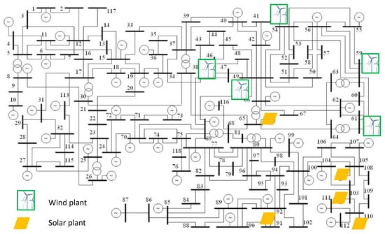
Figure 1.
IEEE 118 bus system one line diagram with a focus on the buses where RES plants are located [].
The feasible phase shift angles belong to the interval , while the minimum and the maximum bus voltage at all the buses have been set, respectively, equal to 0.94 p.u. and 1.06 p.u.
The redispatching costs considered for the DGUs have been set to AMU/MW (Arbitrary Monetary Unit). A more precise selection of the costs can be performed considering the markets, the type of generator, the cost of the fuel, etc., while the RESU curtailment has been strongly penalized with AMU/MW. Finally, the costs related to the relaxing variables have been set very high, i.e., AMU/MW for all the lines of IEEE 118 bus system.
The set of contingencies considered in the simulations is composed of the N-1 outages related to all the lines (excluding radial connections) with an initial active power flow higher than a threshold (set to 150 MW in the present work).
In line with [], the forecast errors for renewable injections are modeled as a beta distribution centered on the mean forecast error. Unless differently specified, the standard deviations for the forecast error distributions of aggregated renewable injections over a 24-h forecast horizon are equal to of the rated power of each injection.
As far as the correlation among forecast errors are concerned, a Toeplitz matrix is considered with a generating vector linearly decreasing from 1 to 0.1 with steps of width 0.14.
4.2. Simulation Scenarios
This section describes the simulation scenarios for validating the linearization techniques (concerning the AC power flow equations and the PST modeling) and for applying the proposed two-stage formulation.
Table 5 summarizes the simulation scenarios reporting for each of them the denomination (ID), a brief description, and its main goals.
Table 5.
Simulation scenarios.
4.3. Validation of the Linearization Techniques
The validation of the linearized models integrated into the proposed control strategy is a fundamental step to guarantee the accuracy of the outcomes of the control itself. The AC power flow linearization described in Section 2.1 has been validated on the IEEE 118 bus system exploiting Matpower as a benchmark. In particular, the function runpf of Matpower has been used []. This function performs a full AC power flow.
The Key Performance Indicator (KPI) used in this comparison has been the Mean Absolute Error (MAE):
where N is the number of samples, is the actual value and is its estimation. In this case, MAE has been evaluated to have information on the error committed on: angles, voltage magnitudes at PQ nodes, active/reactive power injections at PV nodes, and active/reactive power flows.
To validate the PST modeling described in Section 2.2, several simulations have been performed, including a PST in series with lines 30–17. These tests have been executed varying the phase shift (). Again the benchmark exploited has been the DC load flow of Matpower (rundcpf function []), while the KPI has been the Mean Absolute Percentage Error (MAPE), defined as:
where all the quantities involved have been already defined for MAE in Equation (83). In this case, MAPE has been computed on the active power flows.
Table 6 reports the errors in terms of MAE. Figure 2 shows the results related to the approximation of the voltage at PQ nodes, the reactive power at PV nodes, and the reactive power flows. In all these figures, the output of the proposed procedure is depicted in red, while the benchmark is represented in blue.
Table 6.
KPI for the AC power flow linearization.
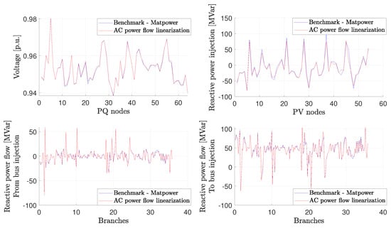
Figure 2.
Results of the AC power flow linearization—Comparison with benchmark.
As seen from the KPIs evaluated in Table 6 and the plots reported in Figure 2, the results are very satisfactory, confirming that this linearization procedure can be exploited within the presented two-stage strategy.
Table 7 summarizes the results in terms of MAPE for the approximation of the active power flows with the presence of a PST and for different values of the phase shift.
Table 7.
Results of the approximation of the active power flows with the presence of a PST.
Figure 3 reports the results obtained with a phase shift equal to 20° (in red) and the comparison with the benchmark (in blue).
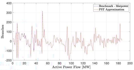
Figure 3.
Results of the active power flows approximation with the presence of a PST—Comparison with benchmark.
4.4. Active Power Control
Two scenarios have been introduced to evaluate the first stage (active power control) of the proposed procedure. In the first scenario (that will be indicated as Scenario APC1), no PSTs have been considered, while in the second (Scenario APC2), a PST is located in series with line 30–17. Therefore, the comparison between the values of the objective function obtained with these two scenarios will help to evaluate the possible contributions of the PSTs. This subsection presents the analysis of the results related to both scenarios.
4.4.1. Scenario APC1
The value of the objective function for this scenario is 2298.93 AMU, while the computational time is 0.117 s (obtained with a processor Intel i7, 16 GB RAM).
Figure 4 reports the results in terms of upward and downward set-point variation of DGUs (in blue and red, respectively) and the curtailment of RESUs (in yellow). It is worth noting that there is no curtailment since it is strongly penalized in the objective function (see Equation (40)) of the active power control.

Figure 4.
Set-point variations of DGUs and RESU curtailment after the active power control−Scenario APC1.
4.4.2. Scenario APC2
This scenario aims to analyze the possible benefits related to the exploitation of PSTs in operating and economic terms for the optimal redispatching.
The value of the objective function passes from 2298.93 AMU (Scenario A) to 2266.33 AMU, proving that the presence of just one PST already brings an interesting advantage both in economic terms (decrease in the objective function imposing a phase shift equal to −3.20°), and in operational terms (all the constraints are satisfied with smaller variations in the set-points of the DGUs).
Figure 5 shows the results obtained in this scenario regarding variations of the active power set-points for DGUs and RESUs.
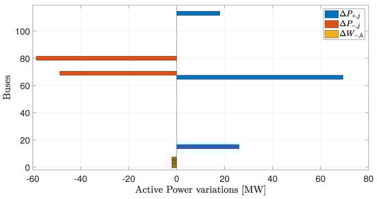
Figure 5.
Set-point variations of DGUs and RESU after the active power control—Scenario APC2.
As can be seen from Figure 5, the presence of a PST allows a lower redispatching of the DGUs (see Figure 4 for Scenario A without PSTs).
Figure 6 illustrates the details of the DGUs. In particular, this figure reports the final set-points of DGUs after the application of the control (in red), the initial set-points of the DGUs (blue line), and the maximum/minimum active power limits (dotted black lines).
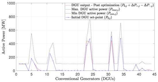
Figure 6.
Active power set-points of DGUs after the active power control—Scenario APC2.
As demonstrated by Figure 5 and Figure 7, there is no curtailment for the RESUs (in fact, red and blue curves overlap in Figure 7) for the same motivations described in Scenario APC1. It is worth noting that in Figure 7, the black dotted line indicates the maximum level of curtailment (downward set-point variation of a RESU) imposed by the probabilistic Constraint (64).
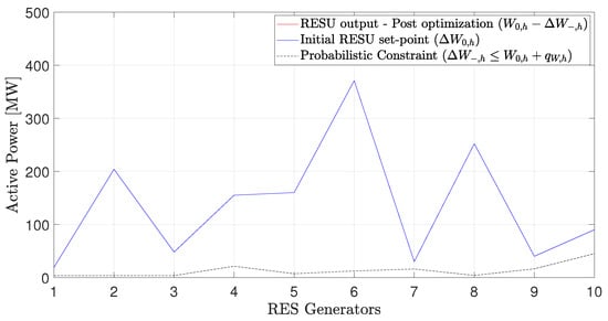
Figure 7.
Active power set-points of RESUs after the active power control—Scenario APC2.
Finally, Figure 8 reports the active power flows on network branches before the application of the control (in state N () and in contingency operation (, )), while Figure 9 shows the same quantities after the active power control (expected power flows in state N (), and in case of contingencies ()). As can be seen from Figure 8, there are some branches with a flow out of the technical limit (see orange arrows), while after the application of the control (see Figure 9), these violations are solved and all the constraints are satisfied.
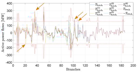
Figure 8.
Active power flows after active power control—Scenario APC2.
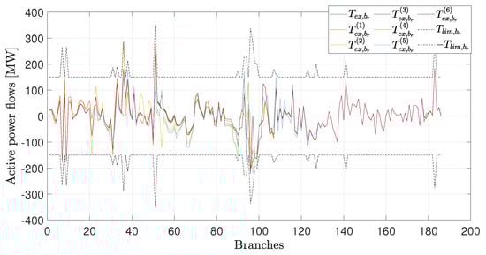
Figure 9.
Active power flows after active power control—Scenario APC2.
4.5. Volt/Var Control
The second stage of the proposed control strategy (Volt/Var control) has been tested after the optimal redispatching presented by the active power control on Scenario APC2. Before applying the Volt/Var control, the working point of the IEEE 188 bus system has been updated according to the output presented in Section 4.4.2 (see scenario VVC in Table 5).
The value of the objective function representing the sum of the modifications in p.u. of the voltage set-points is equal to 0.03 per unit. This means that the network does not need particular interventions to satisfy the constraints related to voltage/reactive power. The calculation time has been 0.079 s (obtained with a processor Intel i7-16 GB RAM). This confirms that the linear formulation allows having a low computational time and that this approach could be interesting with large electrical networks.
Figure 10 shows the results regarding the voltage profile. It is possible to observe the voltage magnitude before the Volt/Var control (in blue), the voltage profile obtained by the optimization (in red), and the voltage limits [0.94–1.06 p.u.] (in dotted black lines).
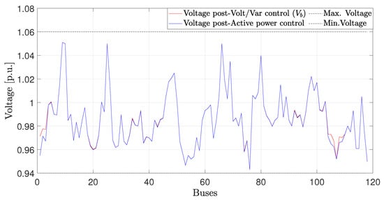
Figure 10.
Results of the Volt/Var control—Voltage profile.
Figure 11 shows the results related to the reactive power of the generators. Moreover, in this case, the output of the optimization is depicted in red, the state before the application of the control is reported in blue, and the technical limits are reported in black. From this figure, it is worth noting that the proposed procedure can be useful in some cases to fulfill the constraints related to the maximum and minimum reactive power. Finally, in this scenario, there are no violations regarding the reactive power flow limits on the network branches.
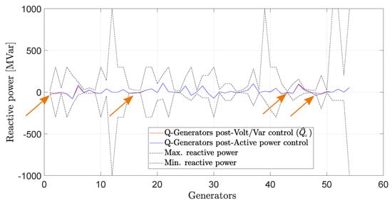
Figure 11.
Results of the Volt/Var control—Reactive power set-points of generators.
5. Conclusions
This paper has proposed a probabilistic preventive control aimed at assuring N-1 security in presence of correlated uncertainties on renewable production and load demand. Exploiting an AC power flow linearization, the procedure is decoupled into two successive linear optimization problems. The first stage concerns active power control. Its goal is to find the optimal conventional generation redispatching, the renewable curtailment, and the PST settings at the minimum cost to assure the fulfillment of N and N-1 security constraints on branch active power flows under forecast uncertainties. The second stage is composed of another linear optimization algorithm, which aims to minimize the adjustments to generators’ set-point voltages to avoid violations at node voltages, reactive power flows, and generator reactive power limits. The approach has been tested by applications to the IEEE 118 bus system.
Future developments may address performance evaluation of the control methodology in the case of large electrical networks, with possible application of decomposition techniques (e.g., Benders decomposition) to further improve the computational speed.
Author Contributions
Conceptualization, E.C. and A.P.; methodology, E.C., A.P. and M.S.; software, F.C., A.P. and M.S.; writing—original draft preparation, M.S.; writing—review and editing, E.C., D.C., S.M. and A.P.; supervision, E.C., D.C. and S.M. All authors have read and agreed to the published version of the manuscript.
Funding
This work has been financed by the Research Fund for the Italian Electrical System in compliance with the Decree of the Minister of Economic Development on 16 April 2018.
Conflicts of Interest
The authors declare no conflict of interest.
References
- Optimal Power System Planning under Growing Uncertainty. Technical Report, CIGRE SC C1 Technical Brochure No. 820. 2020. Available online: https://e-cigre.org/publication/820-optimal-power-system-planning-under-growing-uncertainty (accessed on 6 February 2023).
- Sundar, K.; Nagarajan, H.; Roald, L.; Misra, S.; Bent, R.; Bienstock, D. Chance-Constrained Unit Commitment with N-1 Security and Wind Uncertainty. IEEE Trans. Control. Netw. Syst. 2019, 6, 1062–1074. [Google Scholar] [CrossRef]
- Ghorani, R.; Pourahmadi, F.; Moeini-Aghtaie, M.; Fotuhi-Firuzabad, M.; Shahidehpour, M. Risk-Based Networked-Constrained Unit Commitment Considering Correlated Power System Uncertainties. IEEE Trans. Smart Grid 2020, 11, 1781–1791. [Google Scholar] [CrossRef]
- Peng, C.; Lei, S.; Hou, Y.; Wu, F. Uncertainty management in power system operation. Csee J. Power Energy Syst. 2015, 1, 28–35. [Google Scholar] [CrossRef]
- Roald, L.; Oldewurtel, F.; Van Parys, B.; Andersson, G. Security constrained optimal power flow with distributionally robust chance constraints. arXiv 2015, arXiv:1508.06061. [Google Scholar]
- Roald, L.; Misra, S.; Krause, T.; Andersson, G. Corrective Control to Handle Forecast Uncertainty: A Chance Constrained Optimal Power Flow. IEEE Trans. Power Syst. 2017, 32, 1626–1637. [Google Scholar] [CrossRef]
- Bienstock, D.; Chertkov, M.; Harnett, S. Chance-Constrained Optimal Power Flow: Risk-Aware Network Control under Uncertainty. Siam Rev. 2014, 56, 461–495. [Google Scholar] [CrossRef]
- Bie, P.; Zhang, B.; Li, H.; Wang, Y.; Luan, L.; Chen, G.; Lu, G. Chance-Constrained Real-Time Dispatch with Renewable Uncertainty Based on Dynamic Load Flow. Energies 2017, 10, 2111. [Google Scholar] [CrossRef]
- Kannan, R.; Luedtke, J.R.; Roald, L.A. Stochastic DC optimal power flow with reserve saturation. Electr. Power Syst. Res. 2020, 189, 106566. [Google Scholar] [CrossRef]
- Karangelos, E.; Wehenkel, L. An Iterative AC-SCOPF Approach Managing the Contingency and Corrective Control Failure Uncertainties With a Probabilistic Guarantee. IEEE Trans. Power Syst. 2019, 34, 3780–3790. [Google Scholar] [CrossRef]
- Pena-Ordieres, A.; Molzahn, D.K.; Roald, L.A.; Wachter, A. DC Optimal Power Flow with Joint Chance Constraints. IEEE Trans. Power Syst. 2021, 36, 147–158. [Google Scholar] [CrossRef]
- Franco, J.F.; Ochoa, L.F.; Romero, R. AC OPF for Smart Distribution Networks: An Efficient and Robust Quadratic Approach. IEEE Trans. Smart Grid 2018, 9, 4613–4623. [Google Scholar] [CrossRef]
- You, L.; Ma, H.; Saha, T.K.; Liu, G. Risk-Based Contingency-Constrained Optimal Power Flow with Adjustable Uncertainty Set of Wind Power. IEEE Trans. Ind. Inform. 2022, 18, 996–1008. [Google Scholar] [CrossRef]
- Yang, H.; Zou, B. The Point Estimate Method Using Third-Order Polynomial Normal Transformation Technique to Solve Probabilistic Power Flow with Correlated Wind Source and Load. In Proceedings of the Asia-Pacific Power and Energy Engineering Conference, Shanghai, China, 26–28 March 2012. [Google Scholar] [CrossRef]
- Ciapessoni, E.; Cirio, D.; Massucco, S.; Morini, A.; Pitto, A.; Silvestro, F. Risk-Based Dynamic Security Assessment for Power System Operation and Operational Planning. Energies 2017, 10, 475. [Google Scholar] [CrossRef]
- Pitto, A.; Cirio, D.; Ciapessoni, E. Probabilistic security-constrained preventive redispatching in presence of correlated uncertainties. In Proceedings of the AEIT International Annual Conference, Online, 23–25 September 2020. [Google Scholar] [CrossRef]
- GmbH, G.S. General Algebraic Modeling System (GAMS) Online Documentation. Available online: https://www.gams.com/latest/docs/ (accessed on 6 February 2023).
- Allan, R. Probabilistic a.c. load flow. Proc. Inst. Electr. Eng. 1976, 123, 531–536. [Google Scholar] [CrossRef]
- Verboomen, J.; Van Hertem, D.; Schavemaker, P.H.; Kling, W.L.; Belmans, R. Analytical Approach to Grid Operation With Phase Shifting Transformers. IEEE Trans. Power Syst. 2008, 23, 41–46. [Google Scholar] [CrossRef]
- Verboomen, J.; Papaefthymiou, G.; Kling, W.L.; van der Sluis, L. Use of Phase Shifting Transformers for Minimising Congestion Risk. In Proceedings of the 10th International Conference on Probablistic Methods Applied to Power Systems, Rincon, Puerto Rico, 25–29 May 2008. [Google Scholar]
- Shao, Z.; Zhai, Q.; Wu, J.; Guan, X. Data Based Linear Power Flow Model: Investigation of a Least-Squares Based Approximation. IEEE Trans. Power Syst. 2021, 36, 4246–4258. [Google Scholar] [CrossRef]
- Marinho, N.; Phulpin, Y.; Atayi, A.; Hennebel, M. Modeling Phase Shifters in Power System Simulations Based on Reduced Networks. Energies 2019, 12, 2167. [Google Scholar] [CrossRef]
- Christie, R. Power Systems Test Case Archive. 1999. Available online: https://labs.ece.uw.edu/pstca/pf14/pg_tca14bus.htm (accessed on 6 February 2023).
- Li, Y.; Li, Y.; Sun, Y. Online Static Security Assessment of Power Systems Based on Lasso Algorithm. Appl. Sci. 2018, 8, 1442. [Google Scholar] [CrossRef]
- Holttinen, H.; Söder, L.; Ela, E. Design and Operator of Power Systems with Large Amounts of Wind Power; Technical Report, IEA Wind Task 25, Final Report, Phase I, 2006–2008; VTT Technical Research Centre of Finland: Espoo, Finland, 2009. [Google Scholar]
- Zimmerman, R.D.; Murillo-Sanchez, C.E. Matpower User’s Manual Version 7.1; Power Systems Engineering Research Center (PSerc): Madison, WI, USA, 2020. [Google Scholar]
Disclaimer/Publisher’s Note: The statements, opinions and data contained in all publications are solely those of the individual author(s) and contributor(s) and not of MDPI and/or the editor(s). MDPI and/or the editor(s) disclaim responsibility for any injury to people or property resulting from any ideas, methods, instructions or products referred to in the content. |
© 2023 by the authors. Licensee MDPI, Basel, Switzerland. This article is an open access article distributed under the terms and conditions of the Creative Commons Attribution (CC BY) license (https://creativecommons.org/licenses/by/4.0/).