
Computationally Inexpensive CFD Approach for the Combustion of Sewage Sludge Powder, Including the Consideration of Water Content and Limestone Additive Variations

 , ,
, ,
Abstract
:1. Introduction
1.1. Combustion and Gasification Modelling of Pulverized Sewage Sludge
1.2. Objective of This Paper
2. Materials and Methods
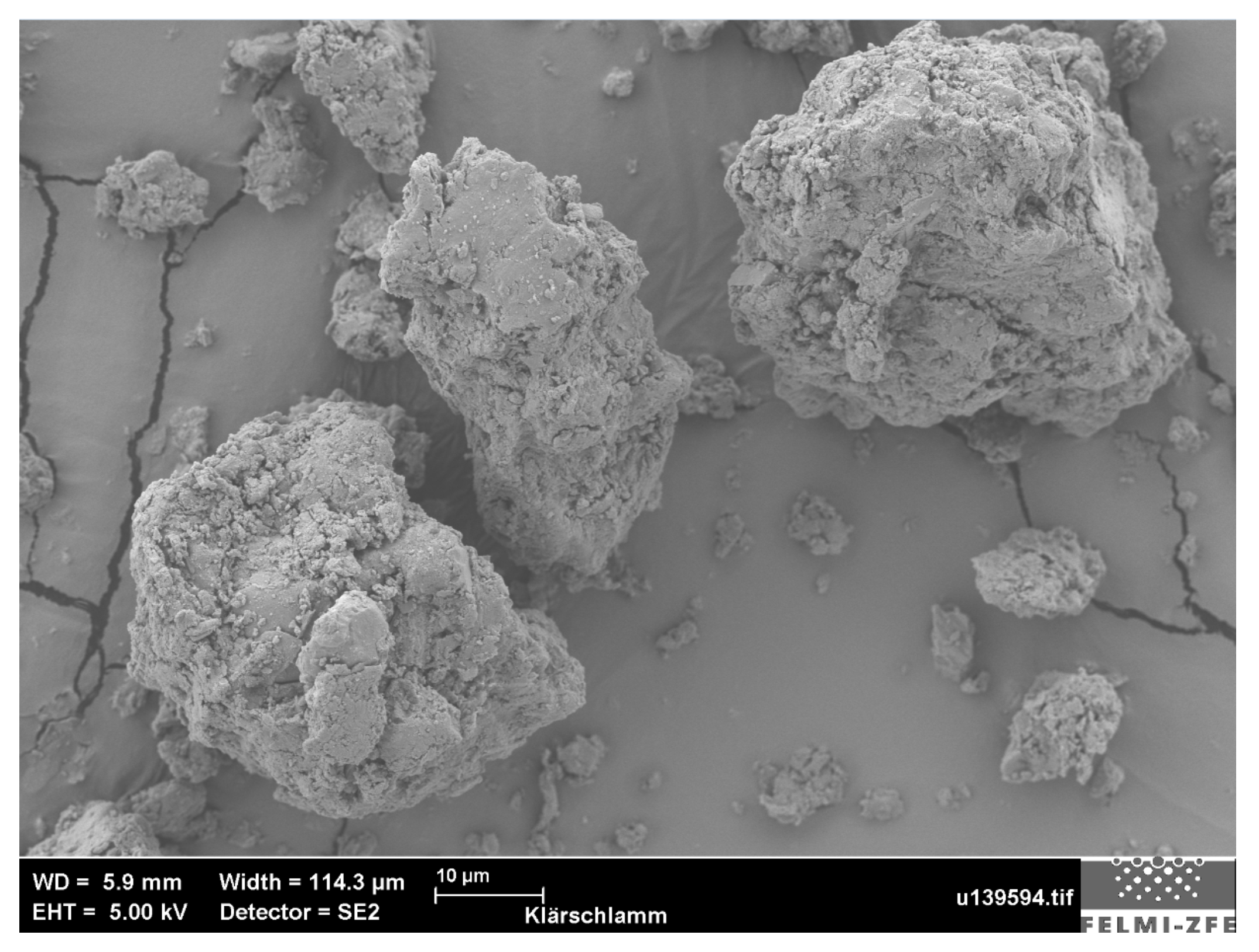
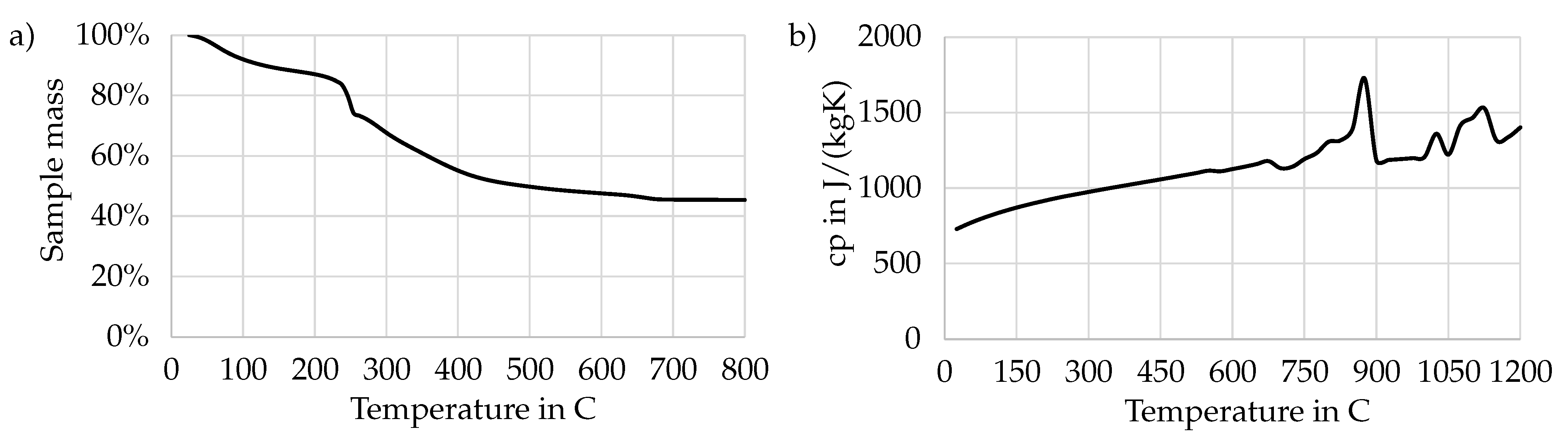
2.1. Material Properties
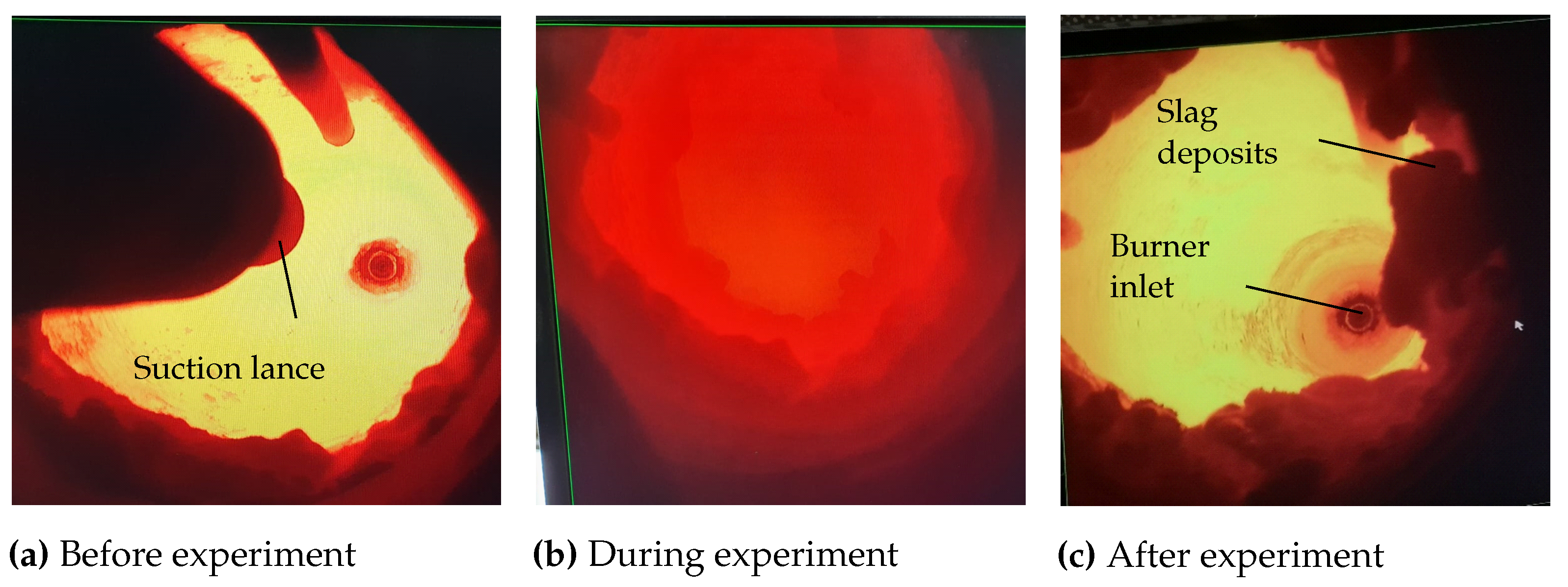
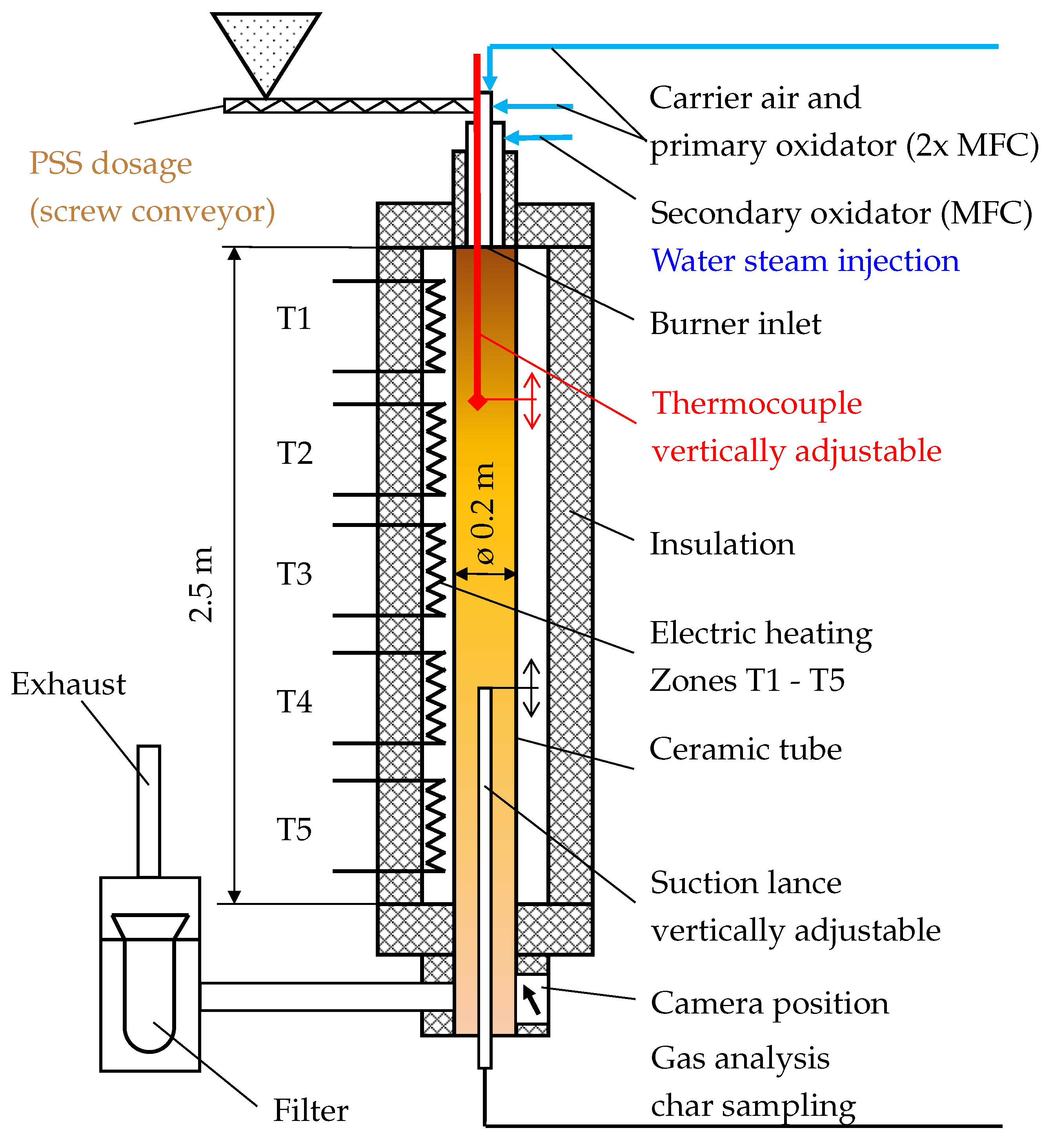
2.2. Experimental Furnace Operation
Measurements
2.3. Numerical Setup
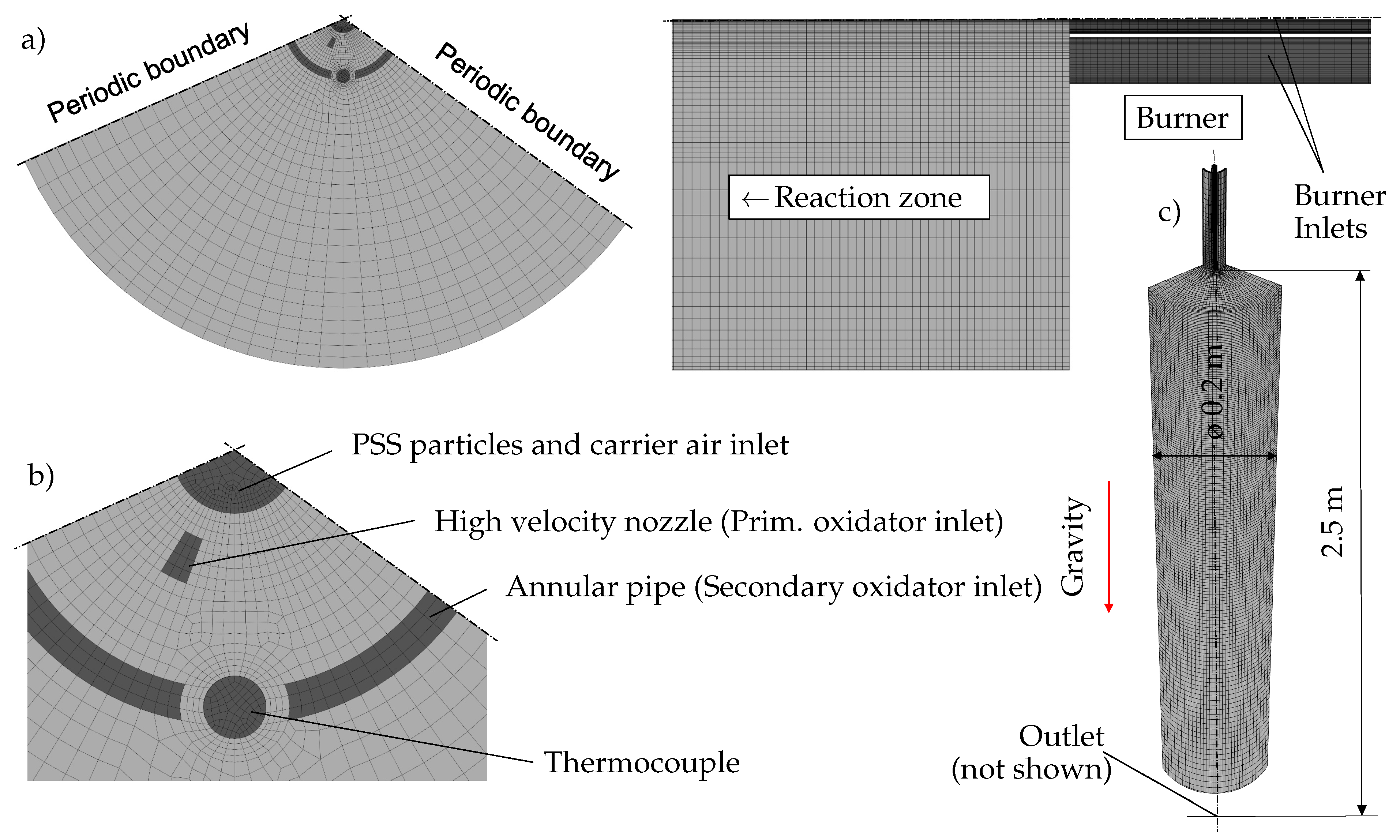
2.3.1. Computational Domain
2.3.2. Particle-Laden Flow
2.3.3. Combustion Modelling
- The volatile fraction of the fuel is very high. Together with water evaporation, close to 60% of the initial particle mass leaves the particle in the form of a released volatile.
- The fixed carbon mass fraction is relatively low in the considered PSS. Therefore, char combustion/gasification also occurs rapidly and can be included in the single mixture fraction, surrogate fuel approach.
- The particles can be safely considered thermally thin. They are of such a small size that no inter-particle temperature gradients need to be considered (Biot number ).
- The high temperatures in the furnace promote fast drying and devolatilization, where the release of distinct off-gasses from a particle cannot meaningfully be distinguished from one another (e.g., CO from CO release). This is further supported by Cui et al. [36], who report that pyrolysis can even happen simultaneously with drying.
- Case 1 deals with the over-stoichiometric combustion of PSS at an ER = 1.2, which should guarantee complete burnout of the fuel.
- Case 2 considers oxygen-enhanced, but sub-stoichiometric combustion (slight gasification) of PSS.
2.3.4. Devolatilization Modelling
2.3.5. Radiation
2.3.6. Boundary Conditions
- Correct HO and N mass fractions to consider water content and fuel nitrogen.
- A H/C and O/C ratio close to that of the original PSS, as given in Table 2.
- The same stoichiometric oxygen demand as is required by the original PSS to obtain consistent inlet velocities (momentum flux) at the burner.
- Volatile and char mass fractions of the particles that match the proximate analysis, otherwise particle track calculations would be based on erroneous mass properties.
- The same adjusted LHV as compared to the original PSS.
- All considered surrogate components are present.
- The H/C and O/C errors are minimized. Therefore, the atomic composition of the surrogate fuel is close to that of the original PSS.
- The stoichiometric air demand error is minimized, which leads to the same inlet momentum flux from the burner.
- The original and the surrogate fuel emitting particle have the same ash mass fraction and LHV.
2.3.7. Implementation of the Limestone Effect
2.3.8. Solution Procedure and Methods
- Solve the oxidator flow only while considering the heated furnace walls until convergence is achieved (turbulent flow field).
- Add DPM particle tracking without considering the chemical reactions.
3. Results and Discussion
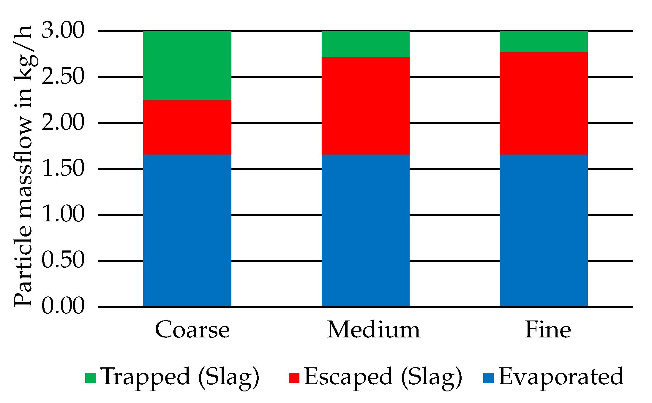
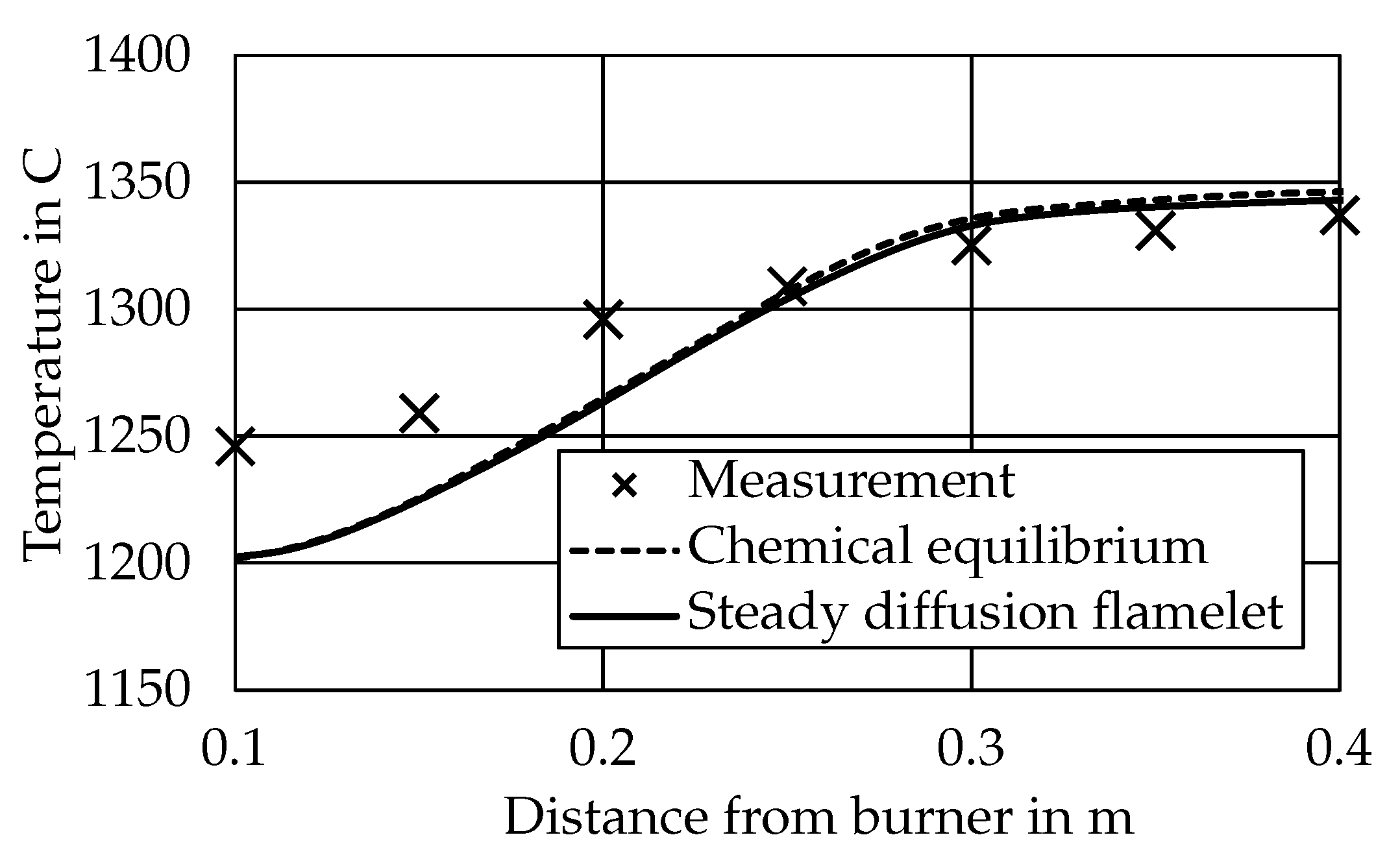
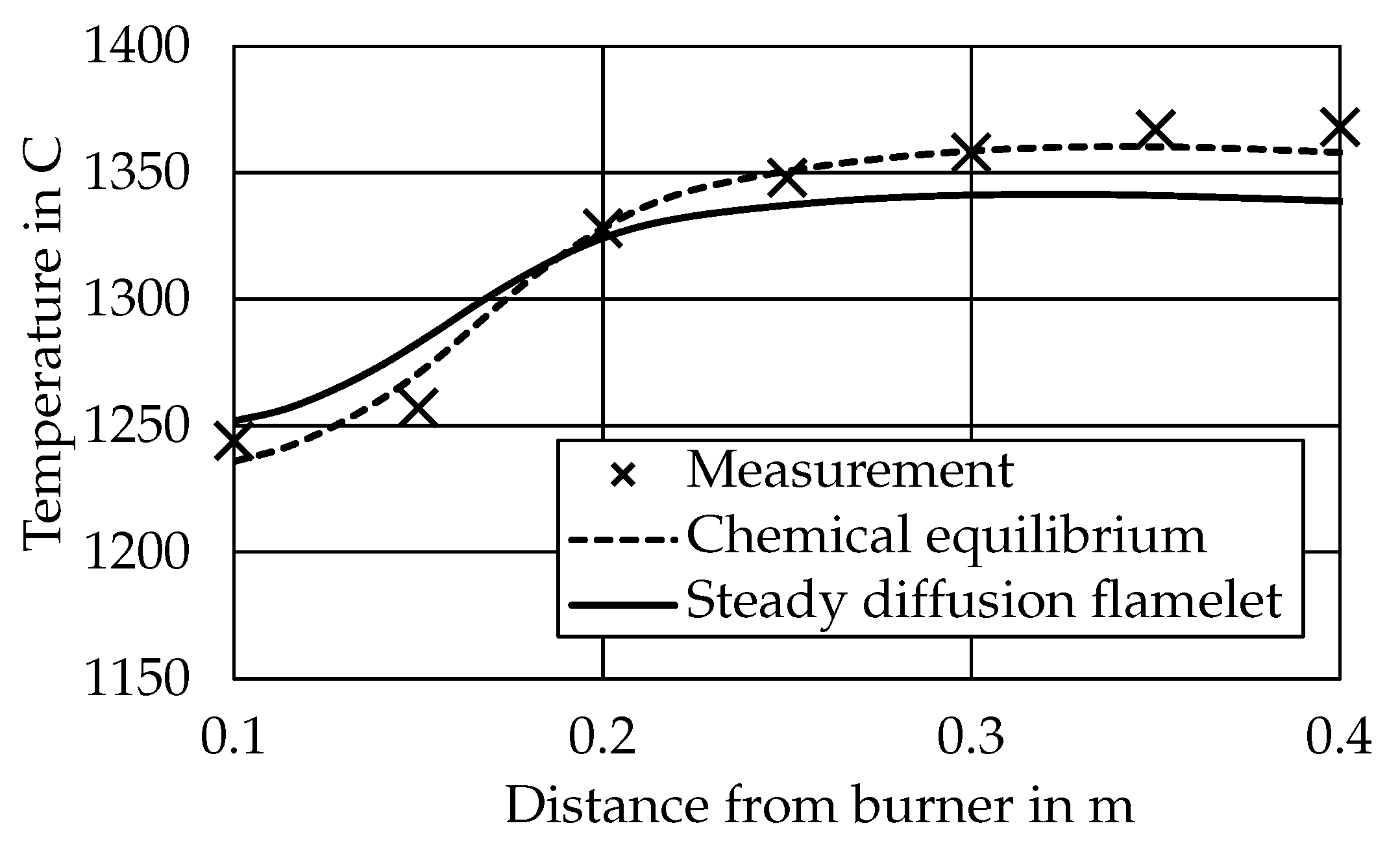
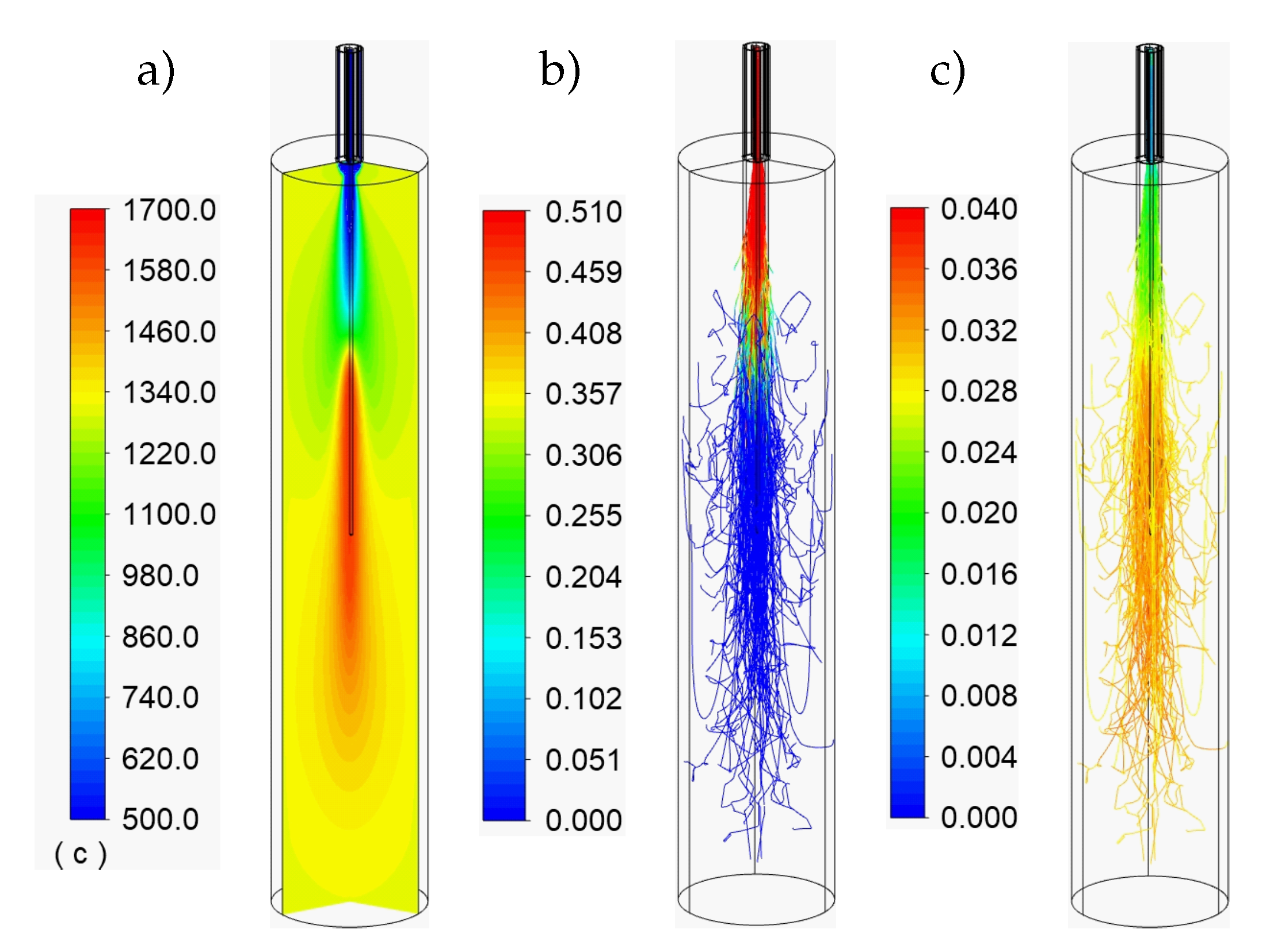
3.1. Particle Conversion and Temperatures
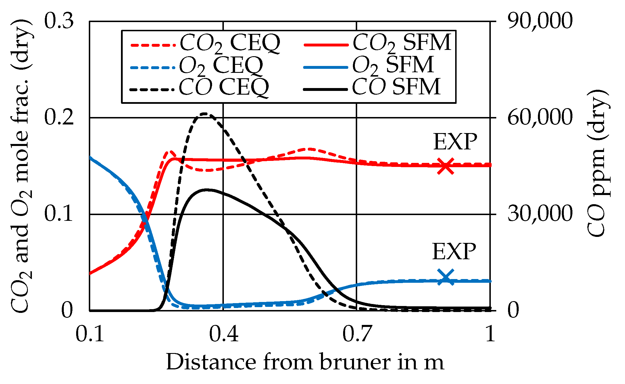
3.2. Species Concentrations
3.2.1. CEQ vs. SFM Approach
- Case 1 is evaluated with the surrogate approach using the SFM model as described above with no modifications.
- Case 2 is evaluated with the surrogate approach using the CEQ model.
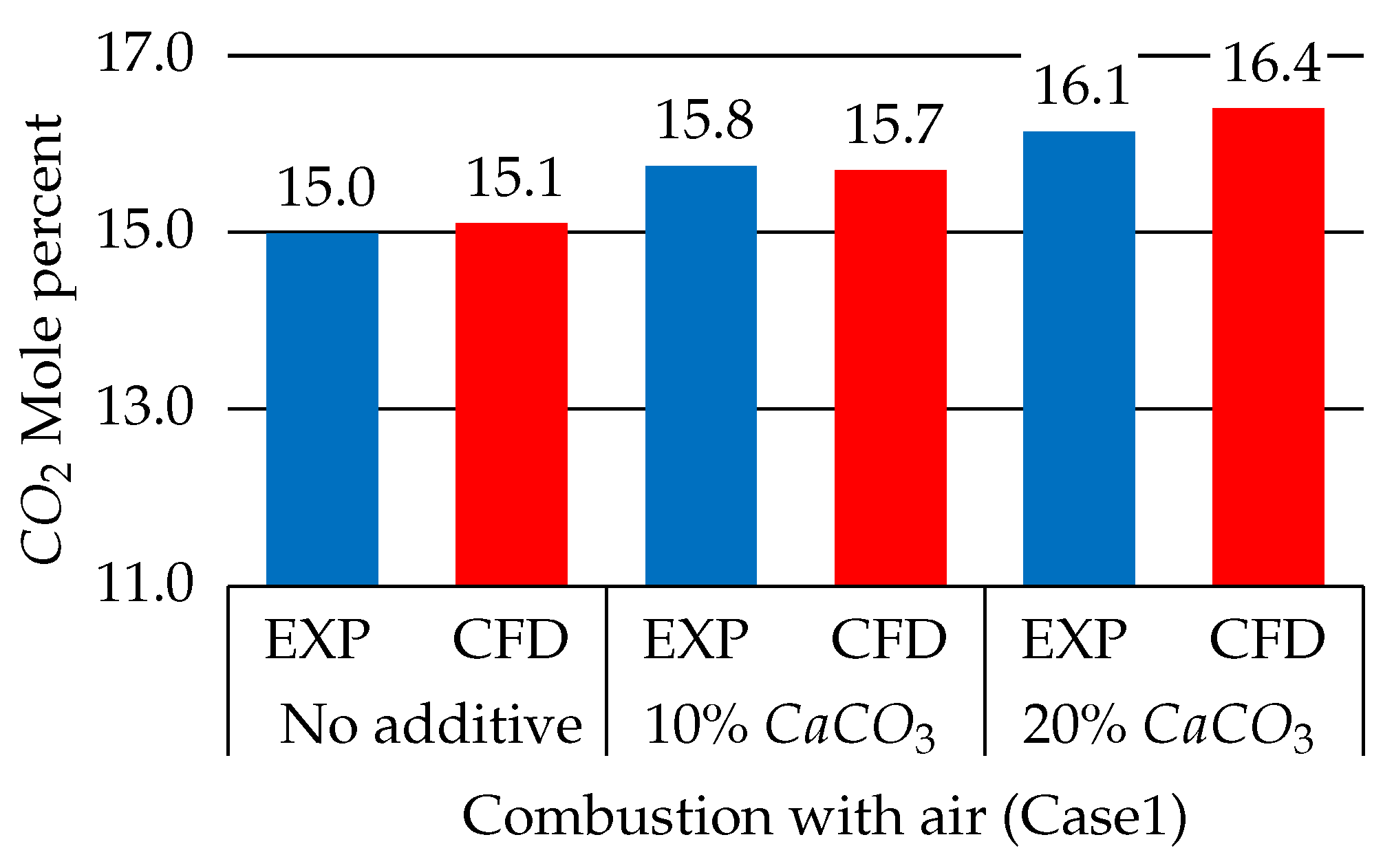
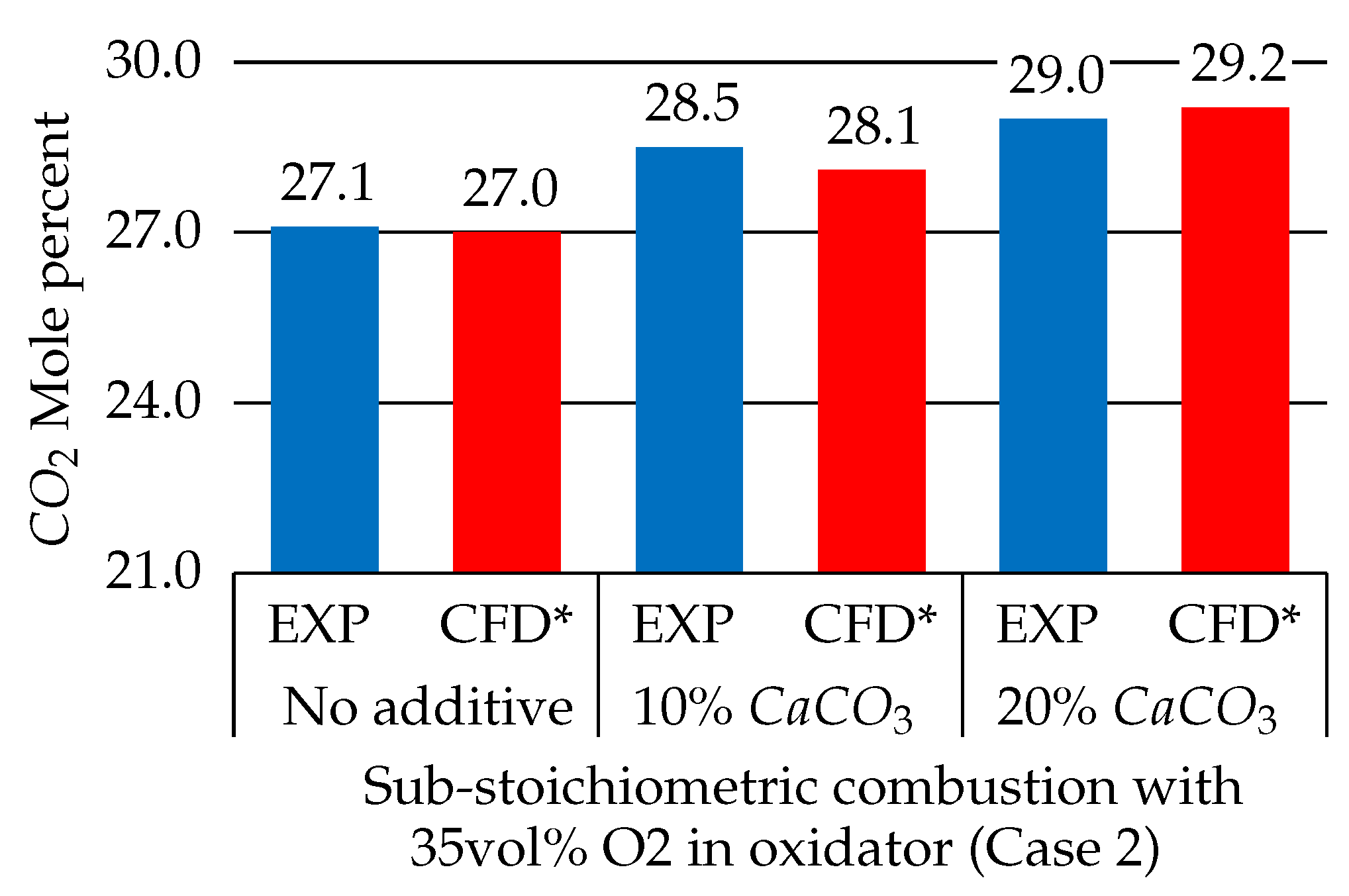
3.2.2. Effect of the Limestone Additive
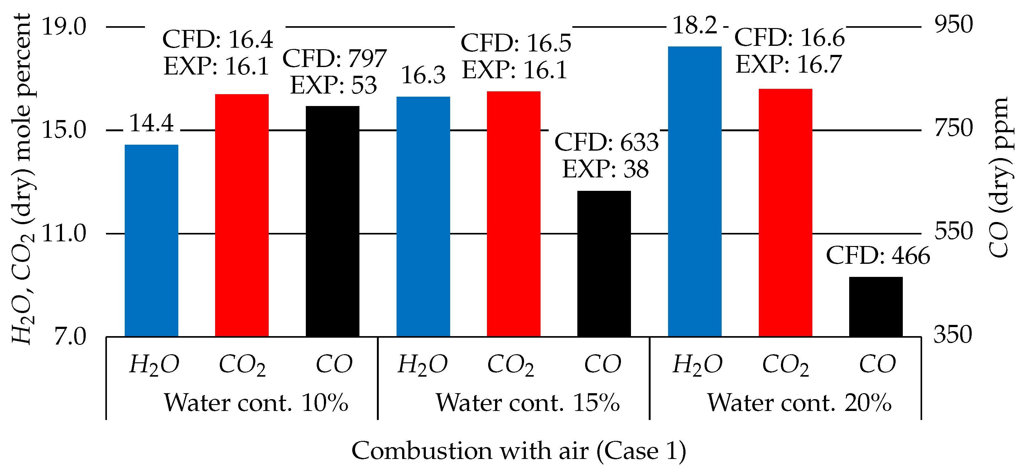
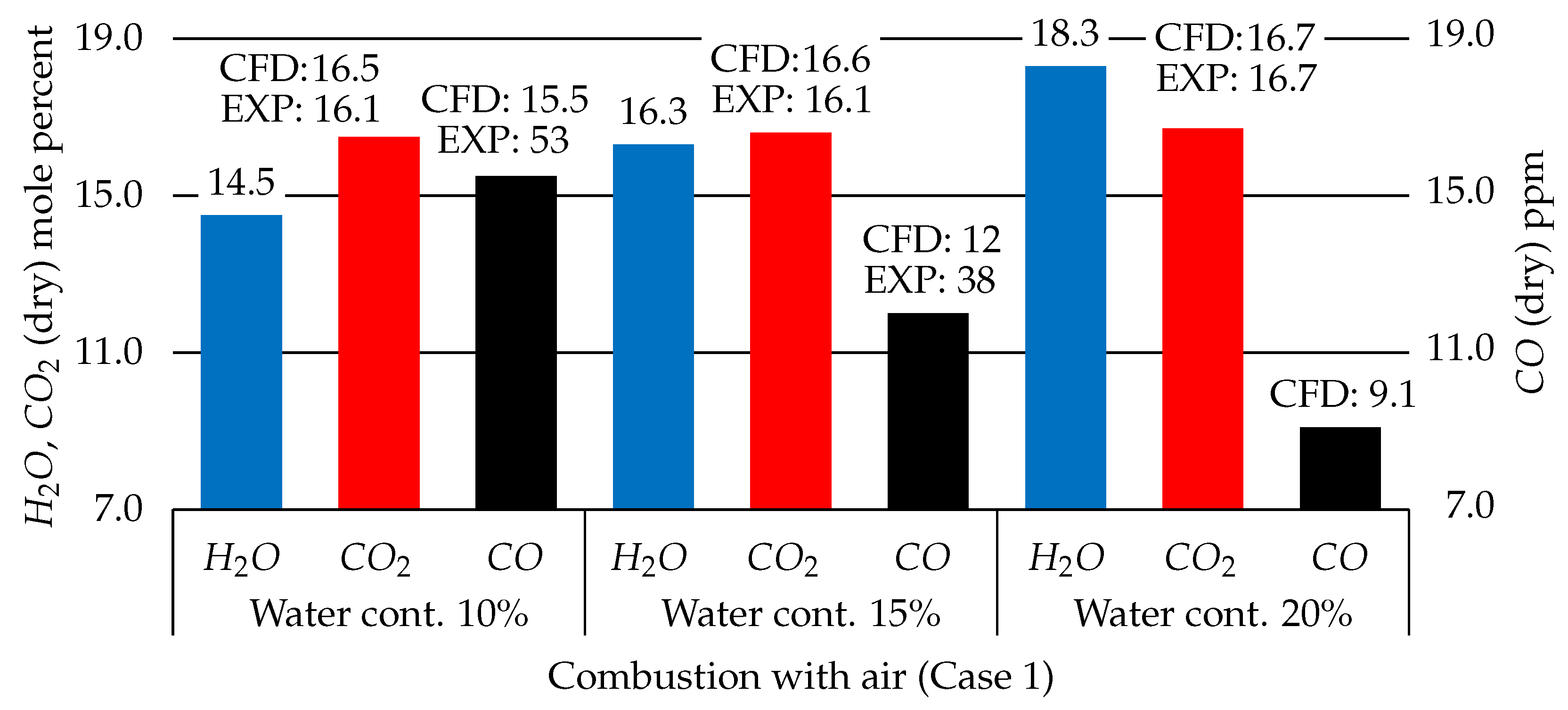
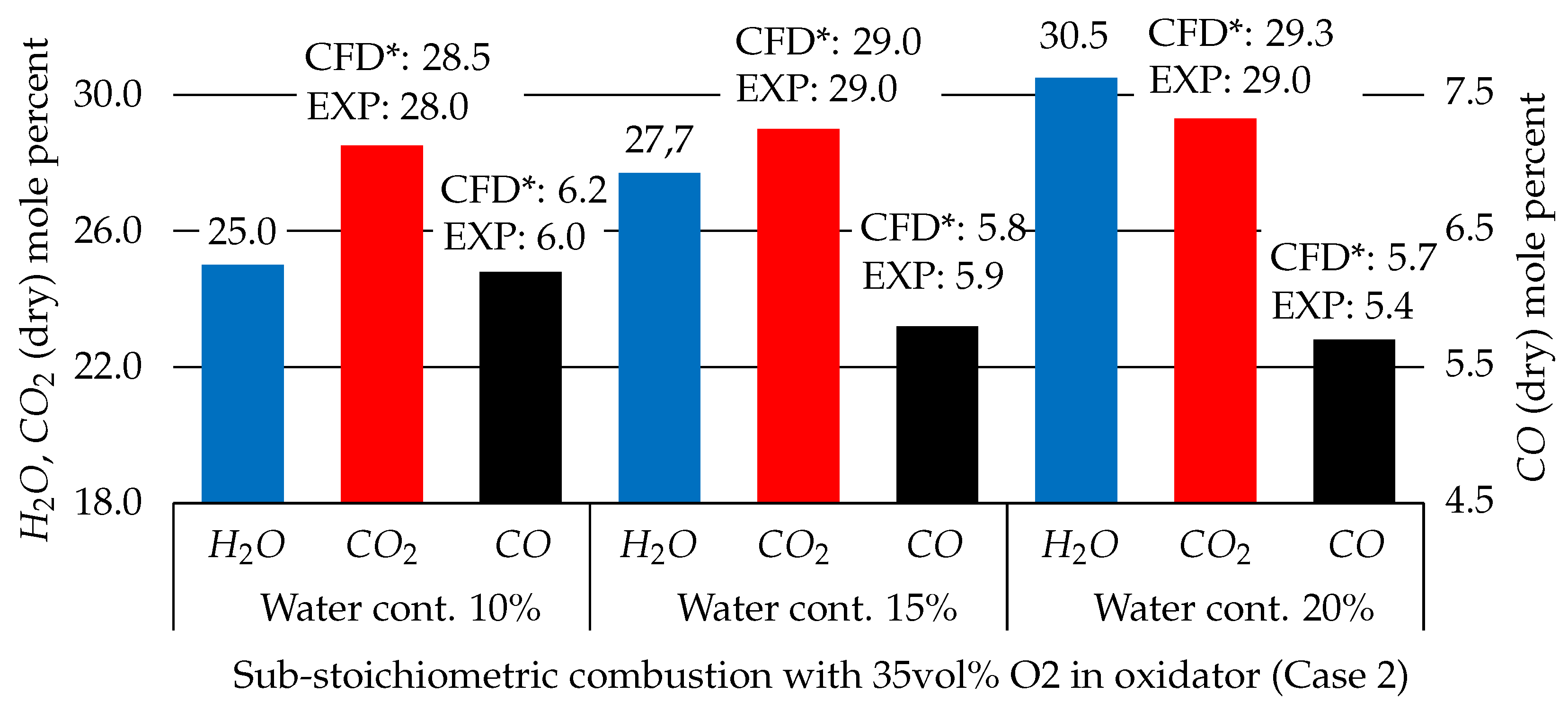
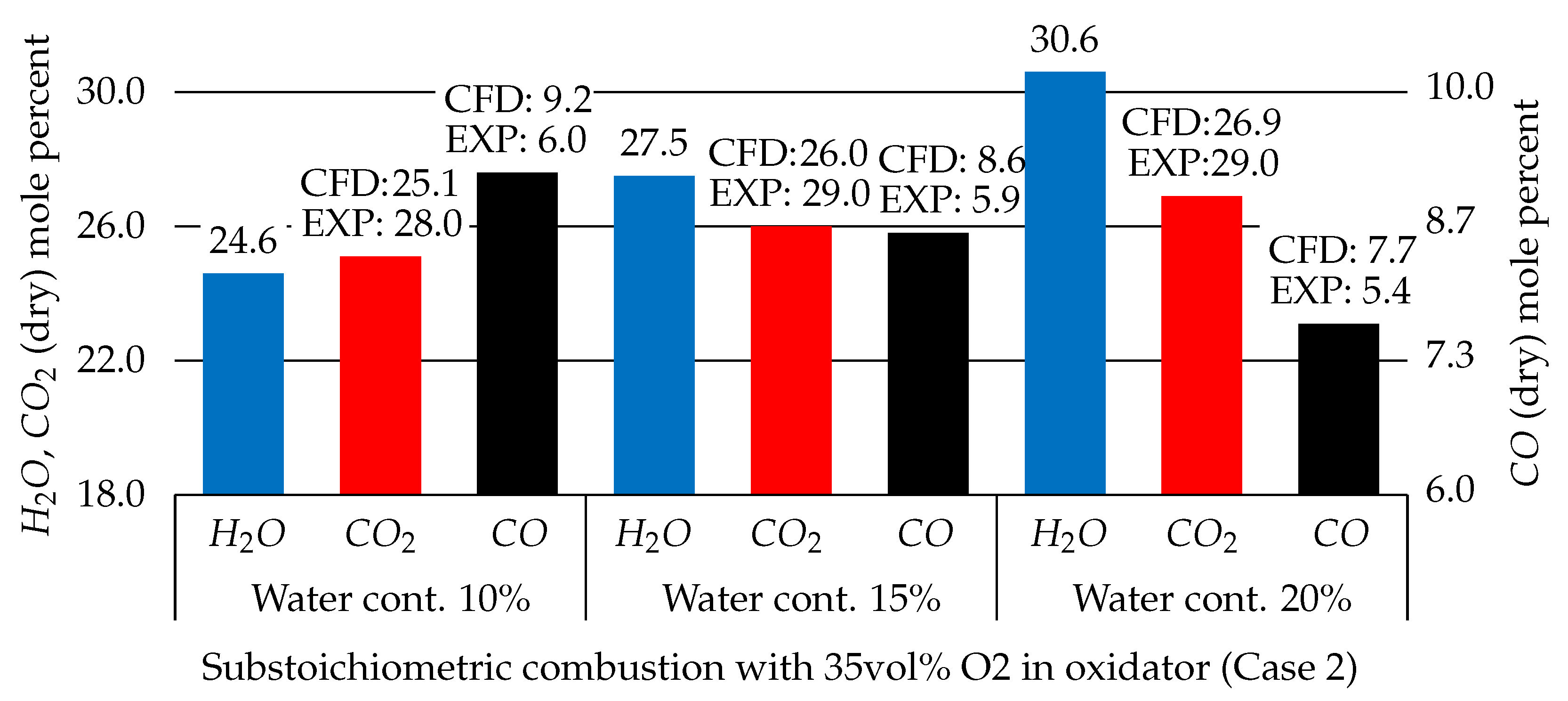
3.2.3. Water Content Effects
4. Conclusions and Outlook
Author Contributions
Funding

Data Availability Statement
Conflicts of Interest
Disclaimer
Abbreviations
| CEQ | Chemical equilibrium model |
| CFD | Computational fluid dynamics |
| DIA | Dynamic image analysis |
| DPM | Discrete phase model |
| EDM | Eddy dissipation model |
| EDC | Eddy dissipation concept |
| ER | Equivalence ratio |
| LCV | Lower calorific value |
| MFC | Mass flow controller |
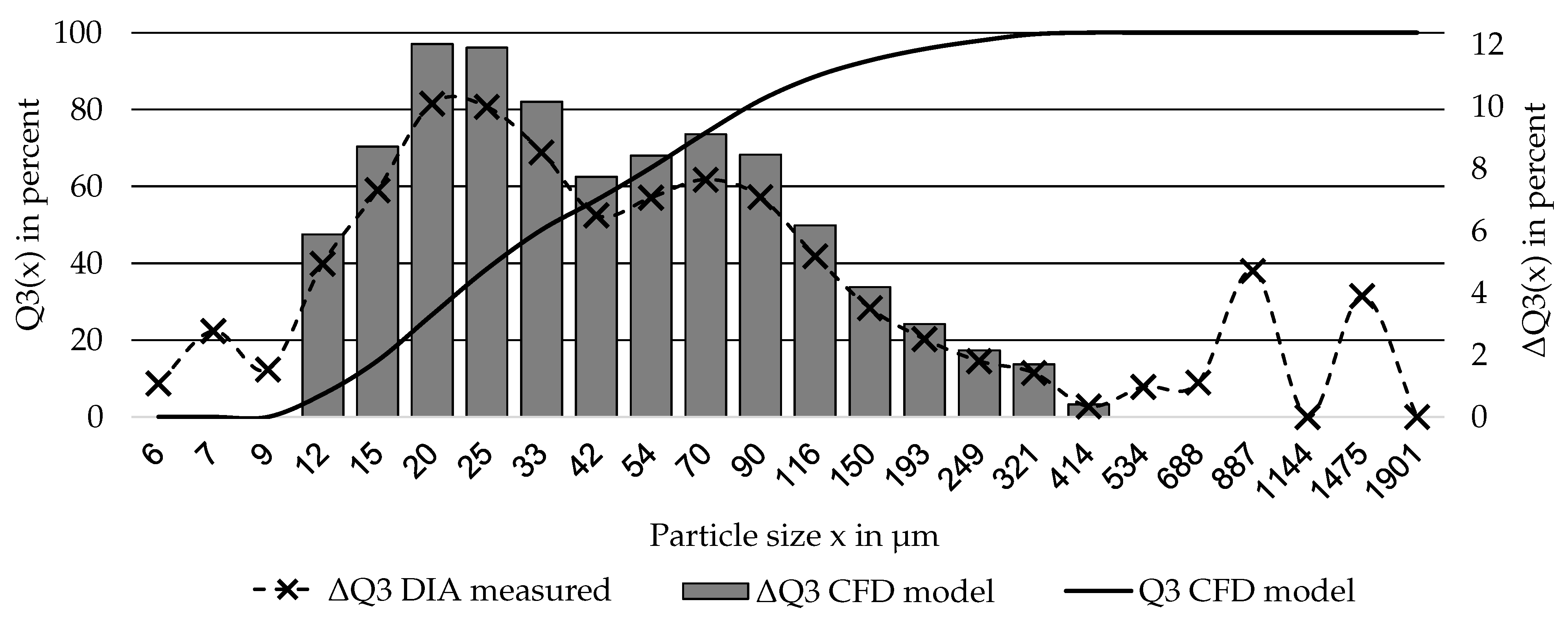
| PSD | Particle size distribution |
| PSS | Pulverized sewage sludge |
| SEM | Scanning electron microscopy |
| RRSB | Rosin–Rammler–Sperling–Bennett (particle size distribution) |
| SFM | Steady diffusion flamelet |
| TC | Thermocouple |
| TGA | Thermogravimetric analysis |
| UDF | User-defined function |
| ar | As received |
| ppm | Parts per million |
| Reynolds number | |
| Biot number | |
| Particle velocity | |
| t | Time |
| Drag force | |
| u | Gas phase velocity |
| g | Gravity |
| Particle density | |
| Gas phase density | |
| Molecular viscosity of the gas phase | |
| Particle diameter | |
| Drag coefficient | |
| Particle mass | |
| Particle specific heat | |
| Particle temperature | |
| Particle volume | |
| Particle surface area | |
| Particle thermal conductivity |
References
- Chanaka Udayanga, W.D.; Veksha, A.; Giannis, A.; Lisak, G.; Chang, V.W.C.; Lim, T.T. Fate and distribution of heavy metals during thermal processing of sewage sludge. Fuel 2018, 226, 721–744. [Google Scholar] [CrossRef]
- Roy, M.M.; Dutta, A.; Corscadden, K.; Havard, P.; Dickie, L. Review of biosolids management options and co-incineration of a biosolid-derived fuel. Waste Manag. 2011, 31, 2228–2235. [Google Scholar] [CrossRef] [PubMed]
- Namkung, H.; Lee, Y.J.; Park, J.H.; Song, G.S.; Choi, J.W.; Choi, Y.C.; Park, S.J.; Kim, J.G. Blending effect of sewage sludge and woody biomass into coal on combustion and ash agglomeration behavior. Fuel 2018, 225, 266–276. [Google Scholar] [CrossRef]
- Stelmach, S.; Wasielewski, R. Co-combustion of dried sewage sludge and coal in a pulverized coal boiler. J. Mater. Cycles Waste Manag. 2008, 10, 110–115. [Google Scholar] [CrossRef]
- Pellegrini, M.; Saccani, C.; Bianchini, A.; Bonfiglioli, L. Sewage sludge management in Europe: A critical analysis of data quality. Int. J. Environ. Waste Manag. 2016, 18, 226. [Google Scholar] [CrossRef]
- Le Quan, M.; Kamyab, H.; Yuzir, A.; Ashokkumar, V.; Hosseini, S.E.; Balasubramanian, B.; Kirpichnikova, I. Review of the application of gasification and combustion technology and waste-to-energy technologies in sewage sludge treatment. Fuel 2022, 316, 123199. [Google Scholar] [CrossRef]
- Atienza-Martínez, M.; Gea, G.; Arauzo, J.; Kersten, S.R.; Kootstra, A.M.J. Phosphorus recovery from sewage sludge char ash. Biomass Bioenergy 2014, 65, 42–50. [Google Scholar] [CrossRef]
- Schoumans, O.F.; Bouraoui, F.; Kabbe, C.; Oenema, O.; van Dijk, K.C. Phosphorus management in Europe in a changing world. Ambio 2015, 44 (Suppl. S2), S180–S192. [Google Scholar] [CrossRef]
- Wang, Y.; Yan, L. CFD based combustion model for sewage sludge gasification in a fluidized bed. Front. Chem. Eng. China 2009, 3, 138–145. [Google Scholar] [CrossRef]
- Yani, S.; Gao, X.; Wu, H. Emission of Inorganic PM 10 from the Combustion of Torrefied Biomass under Pulverized-Fuel Conditions. Energy Fuels 2015, 29, 800–807. [Google Scholar] [CrossRef]
- Feng, C.; Huang, J.; Yang, C.; Li, C.; Luo, X.; Gao, X.; Qiao, Y. Smouldering combustion of sewage sludge: Volumetric scale-up, product characterization, and economic analysis. Fuel 2021, 305, 121485. [Google Scholar] [CrossRef]
- Fletcher, D.F.; Haynes, B.S.; Christo, F.C.; Joseph, S.D. A CFD based combustion model of an entrained flow biomass gasifier. Appl. Math. Model. 2000, 24, 165–182. [Google Scholar] [CrossRef]
- Lin, H.; Ma, X. Simulation of co-incineration of sewage sludge with municipal solid waste in a grate furnace incinerator. Waste Manag. 2012, 32, 561–567. [Google Scholar] [CrossRef] [PubMed]
- Žnidarčič, A.; Seljak, T.; Katrašnik, T. Surrogate model for improved simulations of small-scale sludge incineration plants. Fuel 2020, 280, 118422. [Google Scholar] [CrossRef]
- Žnidarčič, A.; Katrašnik, T.; Zsély, I.G.; Nagy, T.; Seljak, T. Sewage sludge combustion model with reduced chemical kinetics mechanisms. Energy Convers. Manag. 2021, 236, 114073. [Google Scholar] [CrossRef]
- Buchmayr, M.; Gruber, J.; Hargassner, M.; Hochenauer, C. A computationally inexpensive CFD approach for small-scale biomass burners equipped with enhanced air staging. Energy Convers. Manag. 2016, 115, 32–42. [Google Scholar] [CrossRef]
- Buchmayr, M.; Gruber, J.; Hargassner, M.; Hochenauer, C. Performance analysis of a steady flamelet model for the use in small-scale biomass combustion under extreme air-staged conditions. J. Energy Inst. 2018, 91, 534–548. [Google Scholar] [CrossRef]
- Buchmayr, M.; Gruber, J.; Hargassner, M.; Hochenauer, C. Spatially resolved chemical species concentrations above the fuel bed of a small grate-fired wood-chip boiler. Biomass Bioenergy 2016, 95, 146–156. [Google Scholar] [CrossRef]
- Watanabe, J.; Yamamoto, K. Flamelet model for pulverized coal combustion. Proc. Combust. Inst. 2015, 35, 2315–2322. [Google Scholar] [CrossRef]
- Wen, X.; Fan, J. Flamelet modeling of laminar pulverized coal combustion with different particle sizes. Adv. Powder Technol. 2019, 30, 2964–2979. [Google Scholar] [CrossRef]
- Mularski, J.; Modliński, N. Entrained flow coal gasification process simulation with the emphasis on empirical devolatilization models optimization procedure. Appl. Therm. Eng. 2020, 175, 115401. [Google Scholar] [CrossRef]
- Mularski, J.; Pawlak-Kruczek, H.; Modlinski, N. A review of recent studies of the CFD modelling of coal gasification in entrained flow gasifiers, covering devolatilization, gas-phase reactions, surface reactions, models and kinetics. Fuel 2020, 271, 117620. [Google Scholar] [CrossRef]
- Zhu, X.; Zhao, L.; Fu, F.; Yang, Z.; Li, F.; Yuan, W.; Zhou, M.; Fang, W.; Zhen, G.; Lu, X.; et al. Pyrolysis of pre-dried dewatered sewage sludge under different heating rates: Characteristics and kinetics study. Fuel 2019, 255, 115591. [Google Scholar] [CrossRef]
- Mehrabian, R.; Scharler, R.; Obernberger, I. Effects of pyrolysis conditions on the heating rate in biomass particles and applicability of TGA kinetic parameters in particle thermal conversion modelling. Fuel 2012, 93, 567–575. [Google Scholar] [CrossRef]
- Kobayashi, H.; Howard, J.B.; Sarofim, A.F. Coal devolatilization at high temperatures. Symp. Int. Combust. 1977, 16, 411–425. [Google Scholar] [CrossRef]
- Schmid, M.; Beirow, M.; Schweitzer, D.; Waizmann, G.; Spörl, R.; Scheffknecht, G. Product gas composition for steam-oxygen fluidized bed gasification of dried sewage sludge, straw pellets and wood pellets and the influence of limestone as bed material. Biomass Bioenergy 2018, 117, 71–77. [Google Scholar] [CrossRef]
- Al-Abbas, A.H.; Naser, J.; Dodds, D. CFD modelling of air-fired and oxy-fuel combustion in a large-scale furnace at Loy Yang A brown coal power station. Fuel 2012, 102, 646–665. [Google Scholar] [CrossRef]
- Steibel, M.; Halama, S.; Geißler, A.; Spliethoff, H. Gasification kinetics of a bituminous coal at elevated pressures: Entrained flow experiments and numerical simulations. Fuel 2017, 196, 210–216. [Google Scholar] [CrossRef]
- Mu, L.; Wang, S.; Zhai, Z.; Shang, Y.; Zhao, C.; Zhao, L.; Yin, H. Unsteady CFD simulation on ash particle deposition and removal characteristics in tube banks: Focusing on particle diameter, flow velocity, and temperature. J. Energy Inst. 2020, 93, 1481–1494. [Google Scholar] [CrossRef]
- Menter, F.R. Zonal Two Equation k-w Turbulence Models For Aerodynamic Flows. In Proceedings of the AlAA 24h Fuid Dynamics Conference, Orlando, FL, USA, 6–9 July 1993. [Google Scholar] [CrossRef]
- Christ, D. The Effect of Char Kinetics on the Combustion of Pulverized Coal under Oxyfuel Conditions; Diss. RWTH Aachen University: Aachen, Germany, 2013; ISBN 13:978-3-86844-559-6. [Google Scholar]
- Haider, A.; Levenspiel, O. Drag coefficient and Terminal Velocity of Spherical and Nonspherical Particles. Powder Technol. 1988, 58, 63–70. [Google Scholar] [CrossRef]
- Ranz, W.M. Evaporation from drops. Chem. Eng. Prog. 1952, 48, 141–146. [Google Scholar]
- Werther, J.; Ogada, T. Sewage sludge combustion. Prog. Energy Combust. Sci. 1999, 25, 55–116. [Google Scholar] [CrossRef]
- Werther, J.; Ogada, T. Combustion characteristics of wet sludge in a fluidized bed. Fuel 1996, 5, 617–626. [Google Scholar] [CrossRef]
- Cui, H.; Ninomiya, Y.; Masui, M.; Mizukoshi, H.; Sakano, T.; Kanaoka, C. Fundamental Behaviors in Combustion of Raw Sewage Sludge. Energy Fuels 2006, 20, 77–83. [Google Scholar] [CrossRef]
- Bui-Pham, M.; Seshadri, K. Comparison between Experimental Measurements and Numerical Calculations of the Structure of Heptane-Air Diffusion Flames. Combust. Sci. Technol. 1991, 74, 293–310. [Google Scholar] [CrossRef]
- Badzioch, S.; Hawksley, P.G.W. Kinetics of Thermal Decomposition of Pulverized Coal Particles. Ind. Eng. Chem. Process. Des. Dev. 1970, 9, 521–530. [Google Scholar] [CrossRef]
- ANSYS Fluent Theory Guide, Release 2020 R2; ANSYS, Inc.: Canonsburg, PA, USA, 2020.
- Raithby, G.D.; Chui, E.H. A Finite-Volume Method for Predicting a Radiant Heat Transfer in Enclosures with Participating Media. J. Heat. Transf. 1990, 112, 415–423. [Google Scholar] [CrossRef]
- Hottel, H.C.; Cohen, E.S. Radiative Transfer; McGraw-Hill Book Company: New York, NY, USA, 1967. [Google Scholar] [CrossRef]
- Smith, T.F.; Shen, Z.F.; Friedman, J.N. Evaluation of Coefficients for the Weighted Sum of Gray Gases Mode. J. Heat Transf. 1982, 104, 602–608. [Google Scholar] [CrossRef]


| Feature | Comparison to Coal | Mass Fraction |
|---|---|---|
| PSS | ||
| Water content | generally higher for PSS, low in our case due to effective pre-drying | <20% |
| Volatile release | generally higher for PSS, much higher in our case | >40% |
| Fixed carbon | generally lower for PSS, much lower in our case | <4% |
| Ash (slag) | generally higher for PSS, very high in our case | >40% |
| Elementary Analysis | Mass Fraction | Proximate Analysis | Mass Fraction |
|---|---|---|---|
| Daf | |||
| C | 0.508 | Water content | 0.100 |
| H | 0.068 | Volatile matter | 0.409 |
| O | 0.341 | Fixed carbon | 0.041 |
| N | 0.064 | Ash | 0.450 |
| S | 0.019 |
| Heptane42 Component | Mole Fraction Surrogate Fuel No Additive | Mole Fraction Surrogate Fuel 10% CaCO | Mole Fraction Surrogate Fuel 20% CaCO |
|---|---|---|---|
| HO | 0.378 | 0.354 | 0.333 |
| H | 0.030 | 0.028 | 0.026 |
| CO | 0.050 | 0.047 | 0.044 |
| CO | 0.300 | 0.345 | 0.384 |
| CH | 0.030 | 0.028 | 0.026 |
| CH | 0.121 | 0.114 | 0.107 |
| N2 | 0.090 | 0.085 | 0.080 |
| Heptane42 Component | Mole Fraction Surrogate Fuel 10% HO(ar) | Mole Fraction Surrogate Fuel 15% HO | Mole Fraction Surrogate Fuel 20% HO |
|---|---|---|---|
| HO | 0.333 | 0.434 | 0.514 |
| H | 0.026 | 0.027 | 0.027 |
| CO | 0.044 | 0.045 | 0.045 |
| CO | 0.384 | 0.317 | 0.265 |
| CH | 0.026 | 0.027 | 0.027 |
| CH | 0.107 | 0.085 | 0.068 |
| N2 | 0.080 | 0.065 | 0.054 |
| Case 1 Limestone additive variations | ER = 1.2 21vol% O No additive | ER = 1.2 21vol% O 10% CaCO | ER = 1.2 21vol% O 20% CaCO |
| Sewage sludge | 1.00 | 1.00 | 1.00 |
| Limestone | - | 0.10 | 0.20 |
| Feed air | 0.30 | 0.30 | 0.30 |
| Annular pipe | 1.56 | 1.56 | 1.56 |
| High-velocity nozzle | 1.80 | 1.80 | 1.80 |
| Case 2 Limestone additive variations | ER = 0.9 35vol% O No additive | ER = 0.9 35vol% O 10% CaCO | ER = 0.9 35vol% O 10% CaCO |
| Sewage sludge | 1.00 | 1.00 | 1.00 |
| Limestone | - | 0.10 | 0.20 |
| Feed air | 0.30 | 0.30 | 0.30 |
| Annular pipe | 0.45 | 0.45 | 0.45 |
| High-velocity nozzle | 0.90 | 0.90 | 0.90 |
| Case 1 Water content variations | ER = 1.2 21vol% O 10% HO | ER = 1.2 21vol% O 15% HO | ER = 1.2 21vol% O 20% HO |
| Sewage sludge | 1.00 | 1.00 | 1.00 |
| Limestone | 0.20 | 0.20 | 0.20 |
| Feed air | 0.30 | 0.30 | 0.30 |
| Annular pipe | 1.56 | 1.35 | 1.15 |
| High-velocity nozzle | 1.80 | 1.80 | 1.80 |
| Case 2 Water content variations | ER = 0.9 35vol% O 10% HO | ER = 0.9 35vol% O 15% HO | ER = 0.9 35vol% O 20% HO |
| Sewage sludge | 1.00 | 1.00 | 1.00 |
| Limestone | 0.20 | 0.20 | 0.20 |
| Feed air | 0.30 | 0.30 | 0.30 |
| Annular pipe | 0.14 | 0.05 | 0.25 |
| High-velocity nozzle | 1.19 | 1.19 | 0.90 |
Disclaimer/Publisher’s Note: The statements, opinions and data contained in all publications are solely those of the individual author(s) and contributor(s) and not of MDPI and/or the editor(s). MDPI and/or the editor(s) disclaim responsibility for any injury to people or property resulting from any ideas, methods, instructions or products referred to in the content. |
© 2023 by the authors. Licensee MDPI, Basel, Switzerland. This article is an open access article distributed under the terms and conditions of the Creative Commons Attribution (CC BY) license (https://creativecommons.org/licenses/by/4.0/).
Share and Cite
Ortner, B.; Schmidberger, C.; Gerhardter, H.; Prieler, R.; Schröttner, H.; Hochenauer, C. Computationally Inexpensive CFD Approach for the Combustion of Sewage Sludge Powder, Including the Consideration of Water Content and Limestone Additive Variations. Energies 2023, 16, 1798. https://doi.org/10.3390/en16041798
Ortner B, Schmidberger C, Gerhardter H, Prieler R, Schröttner H, Hochenauer C. Computationally Inexpensive CFD Approach for the Combustion of Sewage Sludge Powder, Including the Consideration of Water Content and Limestone Additive Variations. Energies. 2023; 16(4):1798. https://doi.org/10.3390/en16041798
Chicago/Turabian StyleOrtner, Benjamin, Christian Schmidberger, Hannes Gerhardter, René Prieler, Hartmuth Schröttner, and Christoph Hochenauer. 2023. "Computationally Inexpensive CFD Approach for the Combustion of Sewage Sludge Powder, Including the Consideration of Water Content and Limestone Additive Variations" Energies 16, no. 4: 1798. https://doi.org/10.3390/en16041798
APA StyleOrtner, B., Schmidberger, C., Gerhardter, H., Prieler, R., Schröttner, H., & Hochenauer, C. (2023). Computationally Inexpensive CFD Approach for the Combustion of Sewage Sludge Powder, Including the Consideration of Water Content and Limestone Additive Variations. Energies, 16(4), 1798. https://doi.org/10.3390/en16041798