Optimal Control of TBCC Engines in Mode Transition

Abstract

This paper mainly studies the optimal control problem of turbine-based combined cycle (TBCC) engines in the mode-transition stage. Based on the TBCC scheme proposed by Xiamen University, an aerothermodynamic model is established as a verification model for the validity of control laws. To reduce the complexity of control design, a control-oriented linear parameter-varying (LPV) model with Mach number as a scheduling variable is established under a given flight path. The design of mode-transition points and distribution of air-flow-rate among paths during the mode-transition process are transformed into linear quadratic (LQ) optimal control problems for an LPV system under the initial and terminal as well as process constraints. By optimizing the opening of the splitters of the inlet and the fuel flow in each channel, the optimal mode-transition points are found to achieve coordinated control and complete the high-precision thrust tracking during the mode-transition process.

1. Introduction

Hypersonic aircraft have huge military advantages due to their fast combat response and strong battlefield survivability, which will change the rules of the game in future warfare. In terms of civilian use, its development also makes it possible to reach all over the world in one hour. For a hypersonic vehicle that takes off and lands horizontally, the propulsion system is the biggest challenge to be solved [1]. TBCC is a turbine-based combined cycle engine with turbojet mode at low Mach numbers, and ramjet mode at high Mach numbers. It has the advantages of high reliability, low fuel consumption, and high-speed cruise capability, and thus is currently one of the most promising propulsion system solutions [2,3,4]. Since the 1950s, many countries have successively carried out related research on TBCC. The United States’ Revolutionary Turbine Accelerator (RTA) program has determined the development route of two forms of combined power, series, and parallel [5,6]. Trijet proposed by Aerojet realizes a three-power combination by ejecting rockets [7,8]. Japan’s HYPR program has accumulated rich experience in coaxial series turbo-based combination engine [9], and provided corresponding technical support for the research and development of the air-breathing Turbo-Ram expansion cycle engine ATREX [10]. From Sanger project [11] to LAPCAT [12], Europe is constantly trying hypersonic wide-speed propulsion system schemes. China’s Beijing Institute of Power Machinery proposed a turbo-assisted rocket-enhanced ramjet combined cycle engine (TRRE) scheme and carry out relevant research [13,14,15]. Due to the constraints of complexity and cost, modeling is a very important research method. Based on reasonable assumptions and mathematical models of components, the simulation model of the TBCC engine can be used to describe the characteristics of components and the overall performance of TBCC engine [16]. Marshall et al. [17] developed a thermodynamic cycle performance model for TBCC engines. Gamble et al. [18,19] developed a dynamic simulator based on memory-mapped-files technology to demonstrate the mode transition of the TBCC propulsion system. Kong et al. [20] established a calculation model for the overall performance of a hydrogen-cooled turbojet engine. Zhang et al. [21] developed an air-breathing high Mach propulsion system simulation tool (HiMach) for steady state and transient performance analysis of all operating modes of TBCC engines. In recent years, more and more advanced controllers for hypersonic flight vehicles (HFVs) have been designed by researchers, the purpose is to enable the hypersonic vehicles to achieve stable tracking of reference trajectories [22,23,24]. There are few references on the optimal control of TBCC engines.

However, there are still many technical problems in TBCC, such as thrust traps, mode-transition schemes, etc. [25]. Since the TBCC mode-transition point is usually at the upper limit of working Mach number of the turbojet engine and the lower limit of Mach number of the ramjet engine, during the mode-transition process, there may be an unbalanced thrust-drag situation, which will cause the aircraft to continue to decelerate, and cannot provide suitable flow conditions for the normal start of the ramjet engine. In this kind of phenomenon, aircraft cannot complete the transition from low speed to high speed due to the unbalanced thrust and drag is called the thrust trap problem [26]. Increasing the upper limit of the Mach number of the turbine-based engine or lowering the lower limit of the Mach number of the ramjet engine is a theoretical solution to the problem of the TBCC thrust trap. J58 engine adopts the bypass bleed technology to expand the working boundary of the compressor [27]. HYPR90-C engine realizes the control of engine flow state in wide speed range by joint adjustment of multiple geometric adjustment mechanisms [28]. RTA engine realizes mode transition by controlling the mode selection valve and rear variable area ejector after adjusting the first-stage fan [29]. ATREX engine solves the thrust trap problem of TBCC by cooling inlet air through air/hydrogen precooler installed after the inlet [30]. In view of the thrust trap problem of TBCC in the mode-transition between turbojet and ramjet engines, Xiamen University proposed a multi-channel combined power engine scheme called XTER (Xiamen Turbine-based Ejector Ramjet) to trade off the requirements of high-thrust climb and high-specific-impulse cruise [31]. The thrust trap problem is solved by introducing a small-weight, small-sized rocket engine with a high thrust-to-weight ratio. In addition to temporarily increasing the thrust, the ejecting effect of the small rocket can improve the combustion characteristics of the ramjet engine, so as to make it ignite stably. At the same time, due to the reduction in acceleration time, the problem of increased fuel consumption caused by the low specific impulse rocket has been greatly improved [32].

In order to make XTER work along given trajectories within the working range and achieve high-precision thrust tracking, it is necessary to conduct research on the distribution of air-flow-rate among paths and related coordination control of fuel flow in each channel during the mode-transition process. Based on the XTER combined engine scheme, this paper mainly discusses the optimal distribution of air-flow-rate among paths scheme and the coordinated control strategy of each channel during the mode-transition process, so as to achieve high-precision tracking of thrust command. The following tasks have been completed: (1) establishing a component-level aerothermodynamic model of XTER as the basis of control laws synthesis and related verification; (2) obtaining an LPV model (as a simplified model for control design) with Mach number as the scheduling variable by linearizing the component-level model along a given trajectory; and (3) acquiring the optimal distribution of air-flow-rate among paths strategy and mode-transition points by solving the LQ optimal control problem for the LPV system. The main contributions of this paper are: (1) This paper is the first one to use optimization theory to study the distribution of air-flow-rate among paths of the combined inlet, which has not been studied in the current literature. In this paper, the opening of the common inlet splitters is regarded as the control variable, which is written into the control inputs. With this understanding, the optimal control is used to solve the distribution of air-flow-rate among paths and the initial point and terminal point of mode transformation are also unknown variables to be sought, which is a challenging problem that requires both the initial and terminal states to be partially fixed and partially free, and both the initial and terminal independent variables (here the Mach number) are free. (2) For LPV systems, the LQ optimal control problem has not yet mature results for reference, this paper presents a necessary condition that an LQ optimal controller should meet, and a sufficient condition under which an LQ optimal controller is constructed; and (3) The optimal control theory is applied to obtain the best distribution of air-flow-rate among paths as well as the optimal mode-transition points, which will provide a new idea for the design of the control law which regards the opening of the splitters of the common inlet as control variables in the mode-transition stage of TBCC.

The rest of this paper is organized as follows: Section 2 mainly introduces the dynamic modeling methods for the XTER, establishes an LPV model with Mach number as scheduling variable, and then gives a mathematical description of the control problem to be solved; Section 3 focuses on the linear quadratic optimal control problem of LPV systems, some solvable conditions are proposed by using the variational method; Section 4 verifies the coordinated control law of fuel flow in each channel, the optimal distribution of air-flow-rate among paths scheme, and the design method of the optimal mode-transition points through simulations; Section 5 concludes this paper.

2. XTER Modeling and Problem Description

2.1. Aerothermodynamic Modeling

Figure 1 is a structure diagram of XTER. The upper channel is a combined form of Ejector and Ramjet chamber in series, the lower channel is a Scramjet chamber, and the left and right channels are Turbojet engines. The above-mentioned four channels share a common 3D internal turning inlet and a tail nozzle to form a four-channel three-power combined engine.

In order to realize the coordinated control of each channel under the target flight path, it is necessary to carry out aerothermodynamic modeling for XTER. This paper mainly conducts component-level modeling for the combined inlet, Turbojet channel, Ejector-Ramjet channel, and Scramjet channel. The structure of the XTER combined inlet is shown in Figure 2a,b.

In Figure 2a, the upper wall of the entrance of the Turbojet channel is hinged with a splitter to control the cross-sectional area of the entrance, and the opening $\alpha$ of the splitter is a controlled variable. In Figure 2b, the upper wall of the entrance of the Ejector-Ramjet channel is hinged with a splitter to control the cross-sectional area of entrance, and the opening of the splitter $\beta$ is also a controlled variable. The following briefly describes the aerothermodynamic modeling principles of each channel of XTER.

• Combined inlet model

According to the known characteristic data including the flow capture coefficient of each channel, the total pressure recovery coefficient and flight altitude, Mach number, the opening of the splitter of the Turbojet channel, the opening of the splitter of the Ejector-Ramjet channel, the least squares method is used to construct the full-envelope model of the combined inlet. The input variables of the inlet model are flight altitude, Mach number at the entrance, the splitter opening of each channel. The output variables are the total temperature, total pressure, air flow, and Mach number at the outlet of inlet.

• Turbojet channel model

According to the principle of aerodynamics and thermodynamics of a single shaft Turbojet engine, the characteristic curves of typical components such as compressor and turbine, and the working conditions of each component, the models of each component such as the compressor, combustion chamber, turbine, tail nozzle, and rotor shaft of the Turbojet channel are established in turn [33,34].

• Ejector-Ramjet channel model

First, we divide the Ejector-Ramjet channel into the rocket-installation section, rocket-combustion-chamber section, mixing diffuser section, ramjet post-combustion section, and rocket-ramjet nozzle section. Then we establish the Ejector-Ramjet model by using the basic governing equations including the continuity equation, momentum equation, energy equation, and gas state equation [35,36].

• Scramjet channel model

Combined with some physical mechanisms such as the heat release law and wall friction, the models of the isolation section, combustion chamber, and nozzle of the Scramjet engine are constructed by using the influence-coefficient method [37].

When the engines are operating in ramjet mode, it may affect upstream components. We currently concentrate these effects on the inlet. Through the experimental data of the intake port under different back pressure conditions, the boundary of instability is obtained, and the phenomenon of un-starting the inlet is avoided through the instability judgment. Take corresponding measures to ensure the normal operation of the engine before the instability.

In this paper, the inertia effect of some mechanical components such as the splitters in the inlet and the fuel injection devices, the dynamic effect of the rotor, and the volumetric dynamic effect of the combustion chamber are fully considered to achieve accurate models.

• Dynamic characteristics of main components

(a) Dynamic characteristics of the inlet

Considering the inertia effect caused by the mechanical rotation of the splitters, the dynamic characteristics of the inlet are reflected through the following inertia link.

$$T_1\frac{d\alpha \left(t\right)}{dt}+\alpha \left(t\right)={\alpha }_{com}\left(t\right)$$

(1)

$$T_2\frac{d\beta \left(t\right)}{dt}+\beta \left(t\right)={\beta }_{com}\left(t\right)$$

(2)

where $\alpha$ is the splitter opening of Turbojet channel, $\beta$ is the splitter opening of Ejector-Ramjet channel, ${\alpha }_{com}$ and ${\beta }_{com}$ are opening command of the splitters, $T_1$ and $T_2$ are time constants.

(b) Dynamic characteristics of Turbojet channel

The dynamic characteristics of the Turbojet channel are reflected by rotor dynamics effect.

$$P_t-P_c-D\frac{dn\left(t\right)}{dt}=0$$

(3)

where $P_t$ is the turbine power, $P_c$ the compressor power, D the moment of inertia of the rotor shaft, and n the rotor speed.

(c) Dynamic characteristics of Ejector-Ramjet channel

The dynamic characteristics of the Ejector-Ramjet channel are reflected by the dynamic effect of combustion chamber volume [38].

$$\frac{d{T}^{*}}{dt}=\frac{R{T}^{*}}{{\mathrm{C}}_v{V}_b{P}^{*}}\left[m_f\left(H_u{\eta }_b+h_c-\frac{h_t^{*}}{\gamma }\right)+m_0\left(h_a^{*}-\frac{h_t^{*}}{\gamma }\right)-m_1{h}^{*}\left(1-\frac{1}{\gamma }\right)\right]$$

(4)

$$\frac{d{P}^{*}}{dt}=\frac{R{T}^{*}}{V_b}\left(m_0+m_f-m_1\right)+\frac{P^{*}}{T^{*}}\frac{d{T}^{*}}{dt}$$

(5)

where $V_b$ is the volume of the combustion chamber, ${\mathrm{C}}_v$ the specific heat capacity at constant volume, $H_u$ the lower calorific value of fuel, ${\eta }_b$ the combustion efficiency, it is a parameter that could be measured by fitting higher-fidelity models, and is likely to be a function of many other variables in reality. $h_c$ the enthalpy of fuel, $h_a^{*}$ the total enthalpy of incoming flow, $h_t^{*}$ the total enthalpy of outlet; $T^{*}$ and $P^{*}$ are the total temperature and total pressure of the combustion chamber, $m_0$ the air flow, $m_f$ the fuel flow rate, $m_1$ the outlet flow rate, $\gamma$ the gas constant entropy exponent, and R the gas constant of fuel gas.

(d) Dynamic characteristics of fuel injection device

The fuel injection system in the combustion of the rocket or ramjet or Scramjet chambers will result in some dynamic characteristics, which can be described by the following inertia links.

$$T_3\frac{d{m}_f\left(t\right)}{dt}+m_f\left(t\right)=m_{f_{com}}\left(t\right)$$

(6)

where $m_f$ is the fuel flow rate, ${m_f}_{\mathrm{com}}$ the fuel flow command, and $T_3$ a constant.

Combining Equations (1)–(6) and the aerothermodynamic equations, a component-level dynamic model of XTER can be established, which can be used as a verification model for the validity of the control law in this paper. Although many simplifications have been made to XTER, the obtained aerothermodynamic model is still very complex. In order to realize the design of a coordinated control strategy under a given flight path, the aerothermodynamic model needs to be further simplified and a control-oriented dynamic model should be established.

2.2. Control-Oriented LPV Model

The aerothermodynamic model brings challenges to control due to its nonlinear, strong coupling, and time-varying characteristics. Relevant research results have also confirmed that the LPV model is suitable for engine control design because on one hand, it is simple and on the other hand, it still retains the complex features of a time-varying strong coupled nonlinear system [39,40,41].

Given a target path, it is assumed that the expected thrust $F_{ref}$ of the aircraft when flying along the path and the change law of Mach number with time are given as follows.

$$F_{ref}=f\left(Ma\right)$$

(7)

$$Ma=g\left(t\right)$$

(8)

where $F_{ref}$ is the target thrust, $Ma$ the Mach number, and t the time; $f:(M{a}_0,M{a}_f)\to (0,F_{max})$ and $g:(0,\infty )\to (M{a}_0,M{a}_f)$ are smooth functions, $M{a}_0$ and $M{a}_f$ are the corresponding Mach numbers at the initial and terminal points in the path, respectively.

As shown in Figure 3, the working Mach range of XTER is assumed to be $(M{a}_0,M{a}_f)$. $(M{a}_1,M{a}_2)\subset (M{a}_0,M{a}_f)$ and $(M{a}_3,M{a}_4)\subset (M{a}_0,M{a}_f)$ are assumed to correspond to the working speed domain from Turbojet to Ejector-Ramjet and Ejector-Ramjet to Scramjet transition modes, respectively. Among them, $M{a}_1$, $M{a}_2$, $M{a}_3$, $M{a}_4$ satisfying $M{a}_1<M{a}_2<M{a}_3<M{a}_4$ are the Mach numbers of the mode transition points to be designed.

Let $\alpha$ and $\beta$ denote the opening of the splitters of the Turbojet channel and the Ejector-Ramjet channel, respectively, obviously, these two quantities are functions of Mach number and satisfy

$$\alpha \left(Ma\right):\left\{\begin{array}{c}=1,Ma\in (M{a}_0,M{a}_1)\\ \in (0,1),Ma\in (M{a}_1,M{a}_2)\\ =0,Ma\in (M{a}_2,M{a}_f)\end{array}\right.$$

(9a)

$$\beta \left(Ma\right):\left\{\begin{array}{c}=1,Ma\in (M{a}_0,M{a}_3)\\ \in (0,1),Ma\in (M{a}_3,M{a}_4)\\ =0,Ma\in (M{a}_4,M{a}_f)\end{array}\right.$$

(9b)

In (9), 1 means that the channel is fully open, and 0 means that the channel is completely closed.

Next, a control-oriented LPV model for each engine is established based on the flight Mach number. In the mode transition, the states and inputs of the two successive engines operating simultaneously are compounded and expanded to obtain the state and input variables of XTER. Then, superimpose the outputs of the two engines to obtain the output variables of XTER, thus obtaining the LPV model of XTER in the mode transition stage.

• Turbojet’s LPV model

The working Mach range of Turbojet is $(M{a}_0,M{a}_2)$, and its LPV model is described as

$$\left[\begin{array}{c}\Delta {\dot{n}}_1\\ \Delta {\dot{T}}_1^{*}\end{array}\right]=\left[\begin{array}{cc}{a}_1\left(Ma\right)& a_2\left(Ma\right)\\ a_3\left(Ma\right)& a_4\left(Ma\right)\end{array}\right]\left[\begin{array}{c}\Delta n_1\\ \Delta T_1^{*}\end{array}\right]+\left[\begin{array}{cc}{b}_1\left(Ma\right)& b_2\left(Ma\right)\\ b_3\left(Ma\right)& b_4\left(Ma\right)\end{array}\right]\left[\begin{array}{c}\Delta W{f}_1\\ \Delta \alpha \end{array}\right]$$

(10a)

$$\Delta y_1=\Delta F_1=\left[\begin{array}{cc}{c}_1\left(Ma\right)& c_2\left(Ma\right)\end{array}\right]\left[\begin{array}{c}\Delta {\mathrm{n}}_1\\ \Delta T_1^{*}\end{array}\right]$$

(10b)

where $\Delta n_1$ is the increment of the speed of the turbine, $\Delta T_1^{*}$ is the total temperature increment before the turbine, $\Delta W{f}_1$ is the fuel flow increment of the Turbojet channel, $\Delta \alpha$ is the splitter-opening increment of the Turbojet channel, and $\Delta F_1$ is the thrust increment.

• Ejector-Ramjet’s LPV model

Since the boosting effect of the ejection rocket in the Ejector-Ramjet channel is not remarkable, its main function is to improve the combustion characteristics of the Ramjet to make the ignition stable, thus the fuel flow rate of the rocket is set to a fixed value during control-oriented modeling. It can be seen from Figure 3 that the working Mach number of Ejector-Ramjet is $[M{a}_1,M{a}_4]$. Equations (9a) and (9b) show that the opening $\alpha \left(Ma\right)$ only affects the Ejector-Ramjet in the velocity domain $[M{a}_1,M{a}_2]$, and the opening $\beta \left(Ma\right)$ only affects the Ejector-Ramjet in the velocity domain $[M{a}_3,M{a}_4]$; therefore, the LPV model of the Ejector-Ramjet is given in the following two cases.

(b1) When $Ma\in [M{a}_1,M{a}_2]$, the Ejector-Ramjet channel model is described as

$$\left[\begin{array}{c}\Delta {\dot{T}}_2^{*}\\ \Delta {\dot{F}}_2\end{array}\right]=\left[\begin{array}{cc}{a}_5\left(Ma\right)& a_6\left(Ma\right)\\ a_7\left(Ma\right)& a_8\left(Ma\right)\end{array}\right]\left[\begin{array}{c}\Delta T_2^{*}\\ \Delta F_2^{}\end{array}\right]+\left[\begin{array}{cc}{b}_5\left(Ma\right)& b_6\left(Ma\right)\\ b_7\left(Ma\right)& b_8\left(Ma\right)\end{array}\right]\left[\begin{array}{c}\Delta W{f}_2\\ \Delta \alpha \end{array}\right]$$

(11a)

$$\Delta y_2=\Delta F_2$$

(11b)

where $\Delta T_2^{*}$ is the total temperature increment of the Ramjet chamber, $\Delta F_2$ is the thrust increment, $\Delta W{f}_2$ is the fuel flow rate increment of the Ramjet.

(b2) When $Ma\in [M{a}_2,M{a}_4]$, the Ejector-Ramjet channel model is described as

$$\left[\begin{array}{c}\Delta {\dot{T}}_2^{*}\\ \Delta {\dot{F}}_2\end{array}\right]=\left[\begin{array}{cc}{a}_9\left(Ma\right)& a_{10}\left(Ma\right)\\ a_{11}\left(Ma\right)& a_{12}\left(Ma\right)\end{array}\right]\left[\begin{array}{c}\Delta T_2^{*}\\ \Delta F_2\end{array}\right]+\left[\begin{array}{cc}{b}_9\left(Ma\right)& b_{10}\left(Ma\right)\\ b_{11}\left(Ma\right)& b_{12}\left(Ma\right)\end{array}\right]\left[\begin{array}{c}\Delta W{f}_2\\ \Delta \beta \end{array}\right]$$

(12a)

$$\Delta y_2=\Delta F_2$$

(12b)

where $\Delta \beta$ is the increment of the splitter opening of the Ramjet channel.

• Scramjet’s LPV model

The working Mach number of Scramjet is $[M{a}_3,M{a}_f]$, and the Scramjet channel model is described as

$$\left[\begin{array}{c}\Delta {\dot{T}}_3^{*}\\ \Delta {\dot{F}}_3\end{array}\right]=\left[\begin{array}{cc}{a}_{13}\left(Ma\right)& a_{14}\left(Ma\right)\\ a_{15}\left(Ma\right)& a_{16}\left(Ma\right)\end{array}\right]\left[\begin{array}{c}\Delta T_3^{*}\\ \Delta F_3\end{array}\right]+\left[\begin{array}{cc}{b}_{13}\left(Ma\right)& b_{14}\left(Ma\right)\\ b_{15}\left(Ma\right)& b_{16}\left(Ma\right)\end{array}\right]\left[\begin{array}{c}\Delta W{f}_3\\ \Delta \beta \end{array}\right]$$

(13a)

$$\Delta y_3=\Delta F_3$$

(13b)

where $\Delta T_3^{*}$ is the total temperature increment of the Scramjet chamber; $\Delta F_3$ is the thrust increment and $\Delta W{f}_3$ is the fuel flow increment of the Scramjet channel.

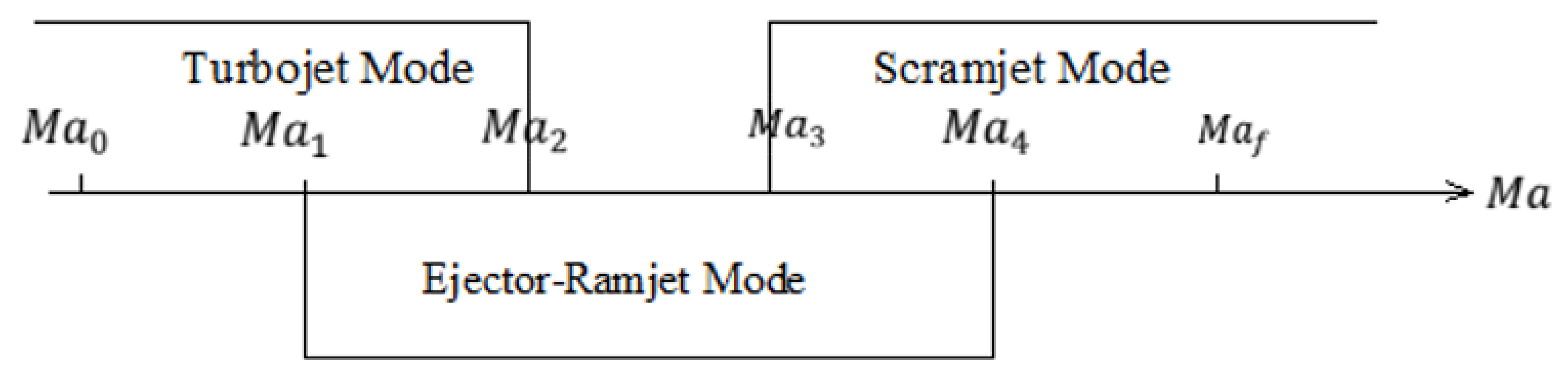
• LPV model in mode transition from Turbojet to Ejector-Ramjet

The working Mach range of this mode transition is $[M{a}_1,M{a}_2]$, in which the Turbojet and Ejector-Ramjet work simultaneously. Therefore, the state input variables of the Turbojet mode and the Ejector-Ramjet mode will be separately combined as the state and input variables in the mode-transition stage, respectively. Similarly, the output in the mode-transition stage is taken as the sum of the outputs of the two channels before and after. The Turbojet to Ejector-Ramjet mode-transition model is described as

$$\begin{array}{c}\left[\begin{array}{c}\Delta {\dot{n}}_1\\ \Delta {\dot{T}}_1^{*}\\ \Delta {\dot{T}}_2^{*}\\ \Delta {\dot{F}}_2\end{array}\right]=\left[\begin{array}{cccc}{a}_1\left(Ma\right)& a_2\left(Ma\right)& 0& 0\\ a_3\left(Ma\right)& a_4\left(Ma\right)& 0& 0\\ 0& 0& a_5\left(Ma\right)& a_6\left(Ma\right)\\ 0& 0& a_7\left(Ma\right)& a_8\left(Ma\right)\end{array}\right]\left[\begin{array}{c}\Delta n_1\\ \Delta T_1^{*}\\ \Delta T_2^{*}\\ \Delta F_2\end{array}\right]+\left[\begin{array}{ccc}{b}_1\left(Ma\right)& 0& b_2\left(Ma\right)\\ b_3\left(Ma\right)& 0& b_4\left(Ma\right)\\ 0& b_5\left(Ma\right)& b_6\left(Ma\right)\\ 0& b_7\left(Ma\right)& b_8\left(Ma\right)\end{array}\right]\left[\begin{array}{c}\Delta W{f}_1\\ \Delta W{f}_2\\ \Delta \alpha \end{array}\right]\hfill \end{array}$$

(14a)

$$\Delta y_{t1}=\Delta y_1+\Delta y_2=\left[\begin{array}{cccc}{c}_1\left(Ma\right)& c_2\left(Ma\right)& 0& 1\end{array}\right]\left[\begin{array}{c}\Delta {\mathrm{n}}_1\\ \Delta T_1^{*}\\ \Delta T_2^{*}\\ \Delta F_2\end{array}\right]$$

(14b)

where $\Delta y_{t1}$ is the total thrust increment.

• LPV model of transition-mode from Ejector-Ramjet to Scramjet

The working Mach range of this mode transition is $[M{a}_3,M{a}_4]$, in which the Ejector-Ramjet and Scramjet work simultaneously. Therefore, the state input variables of the Ejector-Ramjet mode and the Scramjet mode will be separately combined as the state and input variables in the mode-transition stage, respectively. Similarly, the output in the mode-transition stage is taken as the sum of the outputs of the two channels before and after. The Ejector-Ramjet to Scramjet mode-transition model is described as

$$\begin{array}{c}\left[\begin{array}{c}\Delta {\dot{T}}_2^{*}\\ \Delta {\dot{F}}_2\\ \Delta {\dot{T}}_3^{*}\\ \Delta {\dot{F}}_3\end{array}\right]=\left[\begin{array}{cccc}{a}_9\left(Ma\right)& a_{10}\left(Ma\right)& 0& 0\\ a_{11}\left(Ma\right)& a_{12}\left(Ma\right)& 0& 0\\ 0& 0& a_{13}\left(Ma\right)& a_{14}\left(Ma\right)\\ 0& 0& a_{15}\left(Ma\right)& a_{16}\left(Ma\right)\end{array}\right]\left[\begin{array}{c}\Delta T_2^{*}\\ \Delta F_2\\ \Delta T_3^{*}\\ \Delta F_3\end{array}\right]+\left[\begin{array}{ccc}{b}_9\left(Ma\right)& 0& b_{10}\left(Ma\right)\\ b_{11}\left(Ma\right)& 0& b_{12}\left(Ma\right)\\ 0& b_{13}\left(Ma\right)& b_{14}\left(Ma\right)\\ 0& b_{15}\left(Ma\right)& b_{16}\left(Ma\right)\end{array}\right]\left[\begin{array}{c}\Delta W{f}_2\\ \Delta W{f}_3\\ \Delta \beta \end{array}\right]\hfill \end{array}$$

(15a)

$$\Delta y_{t2}=\Delta y_2+\Delta y_3=\left[\begin{array}{cccc}0& 1& 0& 1\end{array}\right]\left[\begin{array}{c}\Delta T_2^{*}\\ \Delta F_2\\ \Delta T_3^{*}\\ \Delta F_3\end{array}\right]$$

(15b)

where $\Delta y_{t2}$ is the total thrust increment.

2.3. Problem Description

There are two mode-transition processes in XTER’s full-speed flight scope: Turbojet to Ejector-Ramjet and Ejector-Ramjet to Scramjet. The optimization principle is the same, so this paper only considers the distribution of air-flow-rate among paths and coordinated control of XTER in the Turbojet to Ejector-Ramjet mode-transition process.

Rewrite the LPV model (14) in the previous section as the following compact form

$$\Delta \dot{x}=A_0\left(Ma\right)\Delta x+B_0\left(Ma\right)\Delta u$$

(16a)

$$\Delta y=C_0\left(Ma\right)\Delta x$$

(16b)

where $\Delta x={(\Delta n_1,\Delta T_1^{*},\Delta T_2^{*},\Delta F_2)}^T$, $\Delta u={(\Delta W{f}_1,\Delta W{f}_2,\Delta \alpha )}^T$, $\Delta y=\Delta y_{t1}$ and $A_0$ is the system matrix, $B_0$ the input matrix, $C_0$ the output matrix.

Combining (16a) with (8), the LPV model with $Ma$ as argument is obtained.

$$\frac{d\Delta x}{dMa}=\frac{d\Delta x}{dt}·\frac{dt}{dMa}=A\left(Ma\right)\Delta x+B\left(Ma\right)\Delta u$$

(17a)

$$\Delta y=C\left(Ma\right)\Delta x$$

(17b)

where $A\left(Ma\right)=A_0\left(Ma\right)·{\left[g^{\prime }\left(t\right){|}_{t=g^{-1}\left(Ma\right)}\right]}^{-1}$, $B\left(Ma\right)=B_0\left(Ma\right)·{\left[g^{\prime }\left(t\right){|}_{t=g^{-1}\left(Ma\right)}\right]}^{-1}$, $C\left(Ma\right)=C_0\left(Ma\right)$.

The following quadratic functional is used to describe the performance index for the optimal flow allocation problem.

$$\begin{array}{c}\mathrm{J}=\frac{1}{2}\Delta y{\left(M{a}_1\right)}^T{F}_1\Delta y\left(M{a}_1\right)+\frac{1}{2}\Delta y{\left(M{a}_2\right)}^T{F}_2\Delta y\left(M{a}_2\right)\hfill \\ +\frac{1}{2}{\int }_{M{a}_1}^{M{a}_2}[\Delta y{\left(Ma\right)}^{T}Q\left(Ma\right)\Delta y\left(Ma\right)+\Delta u^T\left(Ma\right)R\left(Ma\right)\Delta u\left(Ma\right)]dMa\hfill \end{array}$$

(18)

where $Ma\in (M{a}_1,M{a}_2)\subset (M{a}_{01},M{a}_{f1})$, $R\left(Ma\right)$ is a positive definite matrix, $F_1$, $F_2$, $Q\left(Ma\right)$ are positive semi-definite matrix. $M{a}_1$ and $M{a}_2$ are, respectively, the initial and terminal points in the mode transition, and satisfy the following boundary conditions.

$$x_1\left(M{a}_2\right)=0$$

(19a)

$$x_2\left(M{a}_1\right)=0$$

(19b)

where $x_1$ is the state variable of Turbojet channel, and $x_2$ is the state variable of Ejector-Ramjet channel.

By $x=x_e+\Delta x$, (19) is equivalent to

$$\Delta x_1\left(M{a}_2\right)=-x_{1e}\left(M{a}_2\right)$$

(20a)

$$\Delta x_2\left(M{a}_1\right)=-x_{2e}\left(M{a}_1\right)$$

(20b)

where $x_{1e}$ is the state value of $x_1$ at $M{a}_2$, and $x_{2e}$ is the state value of $x_2$ at $M{a}_1$.

The optimal scheme of distribution of air-flow-rate among paths and the coordinated control strategy of each channel during the mode-transition process can be described as

Problem 1.

Find or design $M{a}_1$, $M{a}_2$ and $u=\beta (x,y_d,Ma)$, such that the constraints (17a), (17b), (20a) and (20b) are satisfied and the performance index (18) attains the minimum.

Remark 1.

This problem is essentially an LQ optimal control problem, which has been well solved for general linear time-invariant systems when the initial state is fixed and the terminal state is free. The research object of this paper is the LPV system, and its LQ optimal control problem has not yet mature results for reference. At the same time, the optimization problem proposed in this paper not only requires the initial and terminal states to be partially fixed and partially free, but also requires both the initial and terminal independent variables (here the Mach number) to be free, which is a challenging problem.

3. Main Results

In this section, necessary conditions for the solvability of Problem 1 are derived by using the variational method, and the open-loop LQ optimal controller for the LPV system is obtained. Then, starting from the necessary conditions, a closed-loop LQ optimal controller for the LPV system is obtained by solving a certain differential Ricatti equation.

Theorem 1.

Suppose $\Delta u^{opt}\left(Ma\right)$ is the solution of the optimal control Problem 1, $M{a}_1$ and $M{a}_2$ are the optimal mode-transition points, then there exists $\lambda \left(Ma\right):(M{a}_1,M{a}_2)\to R^4$ such that $\Delta u^{opt}\left(Ma\right)=-R^{-1}\left(Ma\right)B^T\left(Ma\right)\lambda \left(Ma\right)$, and satisfies the following conditions.

(1) 

State equation constraint

$$\frac{d\Delta x}{dMa}=A\left(Ma\right)\Delta x+B\left(Ma\right)\Delta u^{opt}\left(Ma\right)$$

(21)

satisfying the boundary condition (20).

(2) 

Costate equation constraint

$$\dot{\lambda }\left(Ma\right)=-C^T\left(Ma\right)Q\left(Ma\right)C\left(Ma\right)\Delta x-A^T\left(Ma\right)\lambda \left(Ma\right)$$

(22)

where $\lambda =diag\{{\lambda }_1,{\lambda }_2\}$, satisfying the following boundary conditions

$${\lambda }_1\left(M{a}_1\right)=-C_1^T\left(M{a}_1\right)F_1{C}_1\left(M{a}_1\right)\Delta x_1\left(M{a}_1\right)$$

(23a)

$${\lambda }_2\left(M{a}_2\right)=C_2^T\left(M{a}_2\right)F_2{C}_2\left(M{a}_2\right)\Delta x_2\left(M{a}_2\right)$$

(23b)

(3) 

Hamilton function endpoint constraints

$$H\left(M{a}_1\right)-{\left[C_1\left(M{a}_1\right)\Delta x_1\left(M{a}_1\right)\right]}^T{F}_1{C}_1\left(M{a}_1\right)\Delta x_1\left(M{a}_1\right)+{\lambda }_2^T{\dot{x}}_{2e}\left(M{a}_1\right)=0$$

(24a)

$$H\left(M{a}_2\right)+{\left[C_2\left(M{a}_2\right)\Delta x_2\left(M{a}_2\right)\right]}^T{F}_2{C}_2\left(M{a}_2\right)\Delta x_2\left(M{a}_2\right)+{\lambda }_1^T{\dot{x}}_{1e}\left(M{a}_2\right)=0$$

(24b)

where H is the Hamilton function

$$\begin{array}{c}H=\frac{1}{2}\left\{{\left[C\right(Ma)\Delta x(Ma\left)\right]}^{T}Q\left(Ma\right)[C\left(Ma\right)\Delta x\left(Ma\right)]+\Delta u^T\left(Ma\right)R\Delta u\left(Ma\right)\right\}\hfill \\ +{\lambda }^T[A\left(M\mathrm{a}\right)\Delta x+B\left(Ma\right)\Delta u]\hfill \end{array}$$

(25)

Proof of Theorem 1.

Given a target path, consider the LPV system (17) and the expected thrust (7), the performance index (18) can be transformed into

$$\begin{array}{c}J=\frac{1}{2}\left[C_1\left(M{a}_1\right)\right.{\left.\Delta x_1\left(M{a}_1\right)\right]}^T{F}_1\left[C_1\left(M{a}_1\right)\Delta x_1\left(M{a}_1\right)\right]\hfill \\ +\frac{1}{2}{\left[C_2\left(M{a}_2\right)\Delta x_2\left(M{a}_2\right)\right]}^T{F}_2\left[C_2\left(M{a}_2\right)\Delta x_2\left(M{a}_2\right)\right]\hfill \\ +\frac{1}{2}{\int }_{M{a}_1}^{M{a}_2}\left\{{\left[C\right(Ma)\Delta x(Ma\left)\right]}^{T}Q\left(Ma\right)[C\left(Ma\right)\Delta x\left(Ma\right)]\right.\hfill \end{array}$$

(26)

Let

$$\begin{array}{c}\overline{J}=\frac{1}{2}{\left[C_1\left(M{a}_1\right)\Delta x_1\left(M{a}_1\right)\right]}^T{F}_1\left[C_1\left(M{a}_1\right)\Delta x_1\left(M{a}_1\right)\right]\hfill \\ +\frac{1}{2}{\left[C_2\left(M{a}_2\right)\Delta x_2\left(M{a}_2\right)\right]}^T{F}_2\left[C_2\left(M{a}_2\right)\Delta x_2\left(M{a}_2\right)\right]+{\int }_{M{a}_1}^{M{a}_2}\left\{H-{\lambda }^T\Delta \dot{x}\right\}dMa\hfill \\ +{\lambda }_{1a}^T\left(\Delta x_1\left(M{a}_2\right)+x_{1e}\left(M{a}_2\right)\right)+{\lambda }_{2a}^T\left(\Delta x_2\left(M{a}_1\right)+x_{2e}\left(M{a}_1\right)\right)\hfill \end{array}$$

(27)

The variation of the functional $\overline{J}$ is as follows

$$\begin{array}{c}\delta \overline{J}={\left[C_1\left(M{a}_1\right)\Delta x_1\left(M{a}_1\right)\right]}^T{F}_1\left[{\dot{C}}_1\Delta x_1\left(M{a}_1\right)\delta \left(M{a}_1\right)+C_1\left(\delta \left(\Delta x_1\right)+\right.\right.{\left.\left.\Delta {\dot{x}}_1\delta \left(M{a}_1\right)\right)\right]}_{M{a}_1}\hfill \\ +{\left[C_2\left(M{a}_2\right)\Delta x_2\left(M{a}_2\right)\right]}^T{F}_2\left[{\dot{C}}_2\Delta x_2\left(M{a}_2\right)\delta \left(M{a}_2\right)+\right.{\left.C_2\left(\delta \left(\Delta x_2\right)+\Delta {\dot{x}}_2\delta \left(M{a}_2\right)\right)\right]}_{M{a}_2}\hfill \\ +{\left[H-{\lambda }^T\Delta \dot{x}\right]}_{M{a}_2}\delta \left(M{a}_2\right)-[H-{\left.{\lambda }^T\Delta \dot{x}\right]}_{M{a}_1}\delta \left(M{a}_1\right)\hfill \\ +{\int }_{M{a}_1}^{M{a}_2}\left\{\frac{\partial H}{\partial \Delta x}\delta \Delta x+\frac{\partial H}{\partial \Delta u}\delta \Delta u+\frac{\partial H}{\partial \lambda }\delta \lambda -\delta {\lambda }^T\Delta \dot{x}-{\lambda }^T\delta (\Delta \dot{x})\right\}dMa\hfill \\ +\delta {\lambda }_{1a}^T\left(\Delta x_1\left(M{a}_2\right)+x_{1e}\left(M{a}_2\right)\right)+\delta {\lambda }_{2a}^T\left(\Delta x_2\left(M{a}_1\right)+x_{2e}\left(M{a}_1\right)\right)\hfill \\ +{\lambda }_{1a}^T\left(\delta \left(\Delta x_1\right)+\right.{\left.\Delta {\dot{x}}_1\delta \left(M{a}_2\right)+{\dot{x}}_{1e}\delta \left(M{a}_2\right)\right)}_{M{a}_2}\hfill \\ +{\lambda }_{2a}^T{\left(\delta \left(\Delta x_2\right)+\Delta {\dot{x}}_2\delta \left(M{a}_1\right)+{\dot{x}}_{2e}\delta \left(M{a}_1\right)\right)}_{M{a}_1}\hfill \end{array}$$

(28)

where $-{\int }_{M{a}_1}^{M{a}_2}{\lambda }^T\delta (\Delta \dot{x})dMa=-{\left({\lambda }^T\delta (\Delta x)\right)}_{M{a}_1}^{M{a}_2}+{\int }_{M{a}_1}^{M{a}_2}{\dot{\lambda }}^T\delta (\Delta x)dMa$.

Therefore, (28) turns into

$$\begin{array}{c}\delta \overline{J}=\left\{{\left[C_1\left(M{a}_1\right)\Delta x_1\left(M{a}_1\right)\right]}^T{F}_1{C}_1\Delta x_1\left(M{a}_1\right)+{\lambda }_{2a}^T{\dot{x}}_{2e}\left(M{a}_1\right)-H\left(M{a}_1\right)\right\}\delta \left(M{a}_1\right)\hfill \\ +\left\{{\left[C_2\left(M{a}_2\right)\Delta x_2\left(M{a}_2\right)\right]}^T{F}_2{\dot{C}}_2\Delta x_2\left(M{a}_2\right)+{\lambda }_{1a}^T{\dot{x}}_{1e}\left(M{a}_2\right)+H\left(M{a}_2\right)\right\}\delta \left(M{a}_2\right)\hfill \\ +\left\{{\left[C_1\left(M{a}_1\right)\Delta x_1\left(M{a}_1\right)\right]}^T{F}_1{C}_1+{\lambda }_1^T\left(M{a}_1\right)\right\}{\left(\delta \left(\Delta x_1\right)+\Delta \dot{x}\delta \left(M{a}_1\right)\right)}_{M{a}_1}\hfill \\ +\left.{\{C_2\left(M{a}_2\right)\Delta x_2\left(M{a}_2\right)]}^T{F}_2{C}_2-{\lambda }_2^T\left(M{a}_2\right)\right\}{\left(\delta \left(\Delta x_2\right)+\Delta {\dot{x}}_2\delta \left(M{a}_2\right)\right)}_{M{a}_2}\hfill \\ +\left({\lambda }_{1a}^T-\right.n\left.{\lambda }_1^T\left(M{a}_2\right)\right){\left(\delta \left(\Delta x_1\right)+\Delta {\dot{x}}_1\delta \left(M{a}_2\right)\right)}_{M{a}_2}\hfill \\ +\left({\lambda }_{2a}^T+{\lambda }_2^T\left(M{a}_1\right)\right)\left(\delta \left(\Delta x_2\right)+\right.n{\left.\Delta {\dot{x}}_2\delta \left(M{a}_1\right)\right)}_{M{a}_1}\hfill \\ +{\int }_{M{a}_1}^{M{a}_2}\left\{\left[\frac{\partial H}{\partial \Delta x}+{\dot{\lambda }}^T\right]\delta \Delta x+\frac{\partial H}{\partial \Delta u}\delta \Delta u+\left[\frac{\partial H}{\partial \lambda }-{(\Delta \dot{x})}^T\right]\delta \lambda \right\}dMa\hfill \\ +\delta {\lambda }_{1a}^T\left(\Delta x_1\left(M{a}_2\right)+x_{1e}\left(M{a}_2\right)\right)+\delta {\lambda }_{2a}^T\left(\Delta x_2\left(M{a}_1\right)+x_{2e}\left(M{a}_1\right)\right)\hfill \end{array}$$

(29)

From the arbitrariness of the independent variation $\delta \left(M{a}_1\right)$, $\delta \left(M{a}_2\right)$, $\delta {\lambda }_{1a}$, $\delta {\lambda }_{2a}$, $\delta (\Delta x_1\left(M{a}_1\right))$, $\delta (\Delta x_1\left(M{a}_2\right))$, $\delta (\Delta x_2\left(M{a}_1\right))$, $\delta (\Delta x_2\left(M{a}_2\right))$ and $\delta (\Delta x_1\left(Ma\right))$, $\delta (\Delta x_2\left(Ma\right))$, $\forall Ma\in (M{a}_1,M{a}_2)$, the result of Theorem 1 can be obtained. This completes the proof. □

Remark 2.

Theorem 1 gives necessary conditions for the solvability of the LQ optimal control problem for LPV systems, which is similar to the corresponding condition for the LQR optimal control for ordinary linear time-invariant systems [42]. From the expression of the optimal solution $\Delta u^{opt}\left(Ma\right)=-R^{-1}\left(Ma\right)B^T\left(Ma\right)\lambda \left(Ma\right)$, it can be seen that the controller is only open-loop rather than closed-loop. The following theorem will give an optimal controller in the closed-loop form of Problem 1.

Theorem 2.

Assume that the necessary conditions (21), (22) and (24) in Theorem 1 are all satisfied. Suppose there exists $K\left(Ma\right)=diag\{K_1\left(Ma\right),K_2\left(Ma\right)\}$, with $K_1\left(Ma\right),K_2\left(Ma\right)\in R^{2\times 2}$, such that the following conditions hold

$$\begin{array}{c}\dot{K}\left(Ma\right)=-A^T\left(Ma\right)K\left(Ma\right)-K\left(Ma\right)A\left(Ma\right)\hfill \\ +K\left(Ma\right)B\left(Ma\right)R^{-1}\left(Ma\right)B^T\left(Ma\right)K\left(Ma\right)\hfill \\ -C^T\left(Ma\right)Q\left(Ma\right)C\left(Ma\right)\hfill \end{array}$$

(30)

$$K_1\left(M{a}_1\right)=-C_1^T\left(M{a}_1\right)F_1{C}_1\left(M{a}_1\right)$$

(31a)

$$K_2\left(M{a}_2\right)=C_2^T\left(M{a}_2\right)F_2{C}_2\left(M{a}_2\right)$$

(31b)

Then, the closed-loop optimal controller exists and can be expressed as

$$\Delta u^{opt}\left(Ma\right)=-R^{-1}\left(Ma\right)B^T\left(Ma\right)K\left(Ma\right)\Delta x\left(Ma\right)$$

(32)

Furthermore, $M{a}_1$ and $M{a}_2$ can be determined by the constraints (24a) and (24b).

Proof of Theorem 2.

From Theorem 1 one has

$$\Delta u^{opt}\left(Ma\right)=-R^{-1}\left(Ma\right)B^T\left(Ma\right)\lambda \left(Ma\right)$$

(33)

Considering (21)–(23), it is natural to suppose that the costate $\lambda \left(Ma\right)$ has the following structure

$$\lambda \left(Ma\right)=K\left(Ma\right)\Delta x\left(Ma\right)$$

(34)

Substituting (34) into (33), and then substituting into (17), we have

$$\Delta \dot{x}=A\left(Ma\right)\Delta x-B\left(Ma\right)R^{-1}\left(Ma\right)B^T\left(Ma\right)K\left(Ma\right)\Delta x\left(Ma\right)$$

(35)

It is obvious from (22) and (34) that

$$\dot{\lambda }\left(Ma\right)=\dot{K}\left(Ma\right)\Delta x\left(Ma\right)+K\left(Ma\right)\Delta \dot{x}\left(Ma\right)=-C^{T}QC\Delta x-A^{T}K\left(Ma\right)\Delta x\left(Ma\right)$$

(36)

Substituting (35) into (36) yields

$$\begin{array}{c}[\dot{K}\left(Ma\right)+A^T\left(Ma\right)K\left(Ma\right)+K\left(Ma\right)A\left(Ma\right)+C^T\left(Ma\right)QC\left(Ma\right)\hfill \\ -K\left(Ma\right)B\left(Ma\right)R^{-1}{B}^T\left(Ma\right)K\left(Ma\right)]\Delta x\left(Ma\right)=0\hfill \end{array}$$

(37)

The above equation should be true for any $\Delta x\left(Ma\right)$, we have

$$\begin{array}{c}\dot{K}\left(Ma\right)=-A^T\left(Ma\right)K\left(Ma\right)-K\left(Ma\right)A\left(Ma\right)\hfill \\ +K\left(Ma\right)B\left(Ma\right)R^{-1}{B}^T\left(Ma\right)K\left(Ma\right)\hfill \\ -C^T\left(Ma\right)QC\left(Ma\right)\hfill \end{array}$$

(38)

Comparing (23) and (34), it can be obtained that $K\left(Ma\right)$ satisfies the following boundary conditions

$$K_1\left(M{a}_1\right)=-C_1^T\left(M{a}_1\right)F_1{C}_1\left(M{a}_1\right)$$

(39a)

$$K_2\left(M{a}_2\right)=C_2^T\left(M{a}_2\right)F_2{C}_2\left(M{a}_2\right)$$

(39b)

Certainly, $M{a}_1$, $M{a}_2$ should satisfy the constraint (24) from Theorem 1 if they are free to be designed. This completes the proof. □

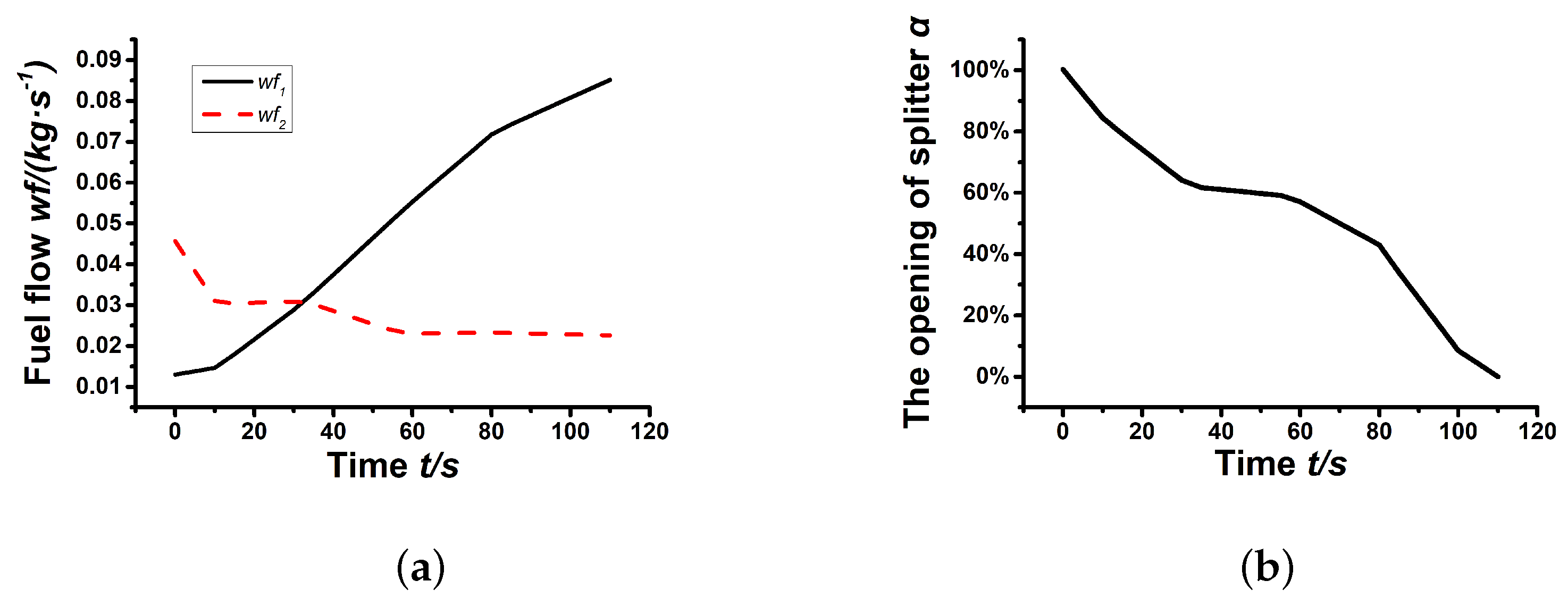
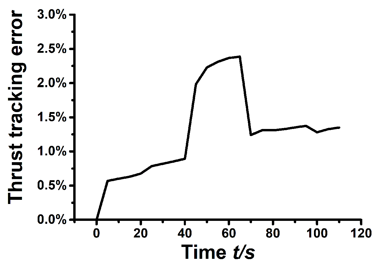
4. Simulation Analysis

This section will verify the optimal scheme of the distribution of air-flow-rate among paths given in Theorems 1 and 2. All simulations are performed on the aerothermodynamics model given in Section 2.1. Suppose that during the mode-transition process, the relative deviation between the real thrust produced by XTER and the expected target thrust is required to be within 10%.

Based on the Gaussian pseudo-spectral track optimization method, Guo et al. [4] completed the optimal design of the TBCC for a hypersonic vehicle cruising at Mach 5 and aiming at the longest cruising range of the hypersonic vehicle for horizontal take-off and landing on the ground, obtained the flight trajectory as shown in Figure 4a,b. The expected thrust for this vehicle is shown in Figure 5. Assume that the power of the vehicle is provided by XTER. The Mach number range of mode transition from Turbojet to Ejector-Ramjet is preset as $[M{a}_{01},M{a}_{f1}]=[2.0,2.5]$. During this transition, the ejection rocket remains open, and the fuel flow rate of the rocket is kept at 0.45 kg/s.

Table 1. Data used for LPV modeling in the mode transition from Turbojet to Ejector-Ramjet.

$\mathit{Ma}$	${\mathit{F}}_{\mathit{e}}$ (N)	${\mathit{F}}_1$/${\mathit{F}}_{\mathit{e}}$	${\mathit{F}}_2$/${\mathit{F}}_{\mathit{e}}$	${\mathit{\alpha }}_{\mathit{e}}$	$\mathit{W}{\mathit{f}}_{1\mathit{e}}$ (kg·s${}^{-1}$)	$\mathit{W}{\mathit{f}}_{2\mathit{e}}$ (kg·s${}^{-1}$)
2.0	2896	100%	0%	100%	0.05	0.012
2.1	3132	80%	20%	80%	0.035	0.014
2.2	3389	60%	40%	60%	0.035	0.029
2.3	3321	40%	60%	40%	0.03	0.052
2.4	3182	20%	80%	20%	0.02	0.072
2.5	2839	0%	100%	0%	0.02	0.085

provides the data at different equilibriums required to establish an LPV model during the mode transition from Turbojet to Ejector-Ramjet, including the Mach number, total thrust, proportion of thrust from the Turbojet and, respectively, Ejector-Ramjet channel, the opening of the splitter in the Turbojet channel, the fuel flow of the Turbojet, and the fuel flow of the Ramjet. With these data as inputs, the value of the equilibrium points are obtained on the established aerothermodynamic model. Then, by imposing a small perturbation at the equilibrium point, the inputs and outputs responses are obtained and used for system identification.

Based on the data in Table 1, we can easily obtain the LPV model in the mode-transition process, which is shown in (17) with the coefficient matrices A, B, and C given by

$$A=\left[\begin{array}{cccc}0.12Ma-1.08& 1.33Ma-3.25& 0& 0\\ -3.08Ma+9.01& 5.229Ma-14.36& 0& 0\\ 0& 0& -35.85Ma-7.80& 191.31Ma-455.4\\ 0& 0& 228.44Ma-431.93& -128.22Ma+286.2\end{array}\right]$$

(40a)

$$B=\left[\begin{array}{ccc}-32.17Ma+37.72& 0& 13.99Ma+1.27\\ -26.39Ma+25.41& 0& 45.79Ma-66.19\\ 0& 151.93Ma-222.54& -385.53Ma+777.6\\ 0& 127.12Ma-167.45& -189.35Ma+358.93\end{array}\right]$$

(40b)

$$C=\left[\begin{array}{cccc}-1.95Ma+5.29& -0.33Ma+0.95& 0& 1\end{array}\right]$$

(40c)

By solving Problem 1 with the method given in Theorem 2, we can obtain the optimal distribution of air-flow-rate among paths scheme, the optimal mode-transition points, and corresponding optimal coordinated control law. Solving the two-point boundary value problem (30) and (31) yields the optimal coordinated control law (32) with $K\left(Ma\right)$ depicted in Figure 6, in which $K\left(Ma\right)$ is of the form

$$K_1\left(Ma\right)=\left[\begin{array}{cc}{k}_{11}\left(Ma\right)& k_{12}\left(Ma\right)\\ k_{13}\left(Ma\right)& k_{14}\left(Ma\right)\end{array}\right]$$

(41a)

$$K_2\left(Ma\right)=\left[\begin{array}{cc}{k}_{21}\left(Ma\right)& k_{22}\left(Ma\right)\\ k_{23}\left(Ma\right)& k_{24}\left(Ma\right)\end{array}\right]$$

(41b)

where $k_{ij}\left(Ma\right)$ ($i=1,2;j=1,2,3,4$) are elements in the matrix $K\left(Ma\right)$.

Furthermore, solving the algebraic Equation (24a) and (24b) gives rise to $Ma1=2.29$ and $Ma2=2.39$.

When making a simulation, the real control law in each channel of XTER is the sum of $u_e\left(Ma\right)+\Delta u^{opt}\left(Ma\right)$, which is detailed in the following.

(I)

Turbojet channel’s fuel flow:

$$W{f}_1\left(Ma\right)=W{f_1}_e\left(Ma\right)+\Delta W{f_1}^{opt}\left(Ma\right)$$

(42)

(II)

Ejector-ramjet channel’s fuel flow:

$$W{f}_2\left(Ma\right)=W{f_2}_e\left(Ma\right)+\Delta W{f_2}^{opt}\left(Ma\right)$$

(43)

(III)

The opening of the splitter:

$$\alpha \left(Ma\right)={\alpha }_e\left(Ma\right)+\Delta {\alpha }^{opt}\left(Ma\right)$$

(44)

The optimal control law in this simulation is shown in Figure 7a,b.

The XTER is accelerated from the ground level by the turbojet engine to Mach 2.29. After then, the turbojet engine is close to the upper limit of its working Mach and difficult to provide enough thrust. The Ejector-Ramjet channel goes to work, the ejection rocket stabilizes the combustion of the ramjet by improving the flow field inside the channel. During the mode-transition process, the proportion of the thrust from the Turbojet channel to the total thrust decreases; meanwhile, the proportion of the thrust from the Ejector-Ramjet channel to the total thrust increases. The distribution of the fuel flow of each channel and the air flow of the inlet also changes accordingly. After accelerating to Mach number 2.39, the mode-transition from the Turbojet to Ejector-Ramjet channel is completed. Figure 7a shows that in the mode-transition interval, the Turbojet channel is gradually closed, and the fuel flow decreases accordingly; the Ejector-Ramjet channel gradually opens, the fuel flow increases, and finally completes the transition from the Turbojet to the Ejector-Ramjet. Figure 7b shows during the transition from the Turbojet to the Ejector-Ramjet, the splitter’s opening gradually decreases. The reduction in the fuel flow of the Turbojet channel reduces its demand for air flow, and the gradual closing of the splitter makes more air flow available to the Ejector-Ramjet channel.

Loading the inputs (42)–(44) into the aerothermodynamic model obtains the real thrust. Compared to the real thrust with the expected thrust, the relative error is shown in Figure 8. It can be seen that during the mode-transition process, the relative error does not exceed 2.5%, which meets the thrust tracking requirements.

5. Conclusions

Based on the XTER project of Xiamen University, this paper discusses the selection of the optimal mode-transition points, optimal distribution of air-flow-rate among paths scheme, and coordinated control strategy of each channel in the process of mode transition. A component-level aerothermodynamic model is derived for the use of verification of control algorithms; meanwhile, some control-oriented LPV models are presented for the purpose of control laws design. In essence, the problem of optimal mode-transition points searching and distribution of air-flow-rate among paths relies on the solvability of LQ optimal control problem for LPV systems. The practice of this paper provides a new idea for the design of the control laws in the mode-transition stage of TBCC.

References

1. Walker, S.; Tang, M.; Mamplata, C. TBCC propulsion for a Mach 6 hypersonic airplane. In Proceedings of the 16th AIAA/DLR/DGLR International Space Planes and Hypersonic Systems and Technologies Conference, Bremen, Germany, 19–22 October 2009. [Google Scholar]
2. Hueter, U.; McClinton, C.; Cook, S. NASA’s advanced space transportation hypersonic program. In Proceedings of the 11th AIAA/AAAF International Conference Space Planes and Hypersonics Systems and Technologies Conference, Orleans, France, 29 September–4 October 2002. [Google Scholar]
3. Liu, J.; Yuan, H.C.; Ge, L. Design and flow characteristics analysis of mode transition simulator for tandem type TBCC inlet. Acta Aeronaut. Astronaut. Sin. 2016, 37, 3675–3684. [Google Scholar]
4. Guo, F.; Zhu, J.F.; You, Y.C. Performance coupling analysis and optimal design of rocket-assisted turbine-based combined cycle engines. Acta Aeronaut. Astronaut. Sin. 2021, 42, 124755. [Google Scholar]
5. Bartolotta, P.; McNelis, N. NASA’s Advanced Space Transportation Program: RTA Project Summary. In Proceedings of the 2001 NASA Seal/Secondary Air System Workshop, Cleveland, OH, USA, 30–31 October 2001; pp. 69–78. [Google Scholar]
6. Mamplata, C.; Tang, M. Technical approach to turbine-based combined cycle: FaCET. In Proceedings of the 45th AIAA/ASME/SAE/ASEE Joint Propulsion Conference & Exhibit, Denver, CO, USA, 2–5 August 2009. [Google Scholar]
7. Siebenhaar, A.; Bogar, T. Integration and vehicle performance assessment of the aerojet “TriJet” combined-cycle engine. In Proceedings of the 16th AIAA/DLR/DGLR International Space Planes and Hypersonic Systems and Technologies Conference, Bremen, Germany, 19–22 October 2009. [Google Scholar]
8. Saunders, J.D.; Stueber, T.J.; Thomas, S.R.; Suder, K.L.; Weir, L.J.; Sanders, B.W. Testing of the NASA Hypersonics Project Combined Cycle Engine Large Scale Inlet Mode Transition Experiment (CCE LlMX). In Proceedings of the 58th Joint Army-Navy-NASA-Air Force (JANNAF) Propulsion Meeting, Cleveland, OH, USA, 25 August 2013. [Google Scholar]
9. Ito, M. International collaboration in super/hypersonic propulsion system research project (HYPR). Aeronaut. J. 2000, 104, 445–451. [Google Scholar] [CrossRef]
10. Sato, T.; Tanatsugu, N.; Naruo, Y.; Omi, J.; Tomike, J.; Nishino, T. Development study on ATREX engine. Acta Astronaut 2000, 47, 799–808. [Google Scholar] [CrossRef]
11. Weingertner, S. SÄNGER-The reference concept of the german hypersonics technology program. In Proceedings of the 5th International Aerospace Planes and Hypersonics Technologies Conference, Munich, Germany, 30 November–3 December 1993. [Google Scholar]
12. Langener, T.; Erb, S.; Steelant, J.; Flight, H. Trajectory simulation and optimization of the LAPCAT MR2 hypersonic cruiser concept. ICAS 2014, 2014, 428. [Google Scholar]
13. Wei, B.X.; Ling, W.H.; Gang, Q.; Wei, X.G.; Qin, F.; He, G.Q. Analysis of key technologies and propulsion performance research of TRRE engine. J. Propuls. Technol. 2017, 38, 298–305. [Google Scholar]
14. Hui, Y.; Jun, M.; Man, Y.; Zhu, S.; Ling, W.; Cao, X. Numerical simulation of variable-geometry inlet for TRRE combined cycle engine. In Proceedings of the 21st AIAA International Space Planes and Hypersonics Technologies Conference, Xiamen, China, 6–9 March 2017. [Google Scholar]
15. Wei, B.X.; Ling, W.H.; Luo, F.; Gang, Q. Propulsion performance research and status of TRRE engine experiment. In Proceedings of the 21st AIAA International Space Planes and Hypersonics Technologies Conference, Xiamen, China, 6–9 March 2017. [Google Scholar]
16. Krouse, C.; Connolly, B.; Gordon, E. Integration of Inlet and Combustor Subsystem Models into a TBCC Engine Performance Model. In Proceedings of the 2022 IEEE Aerospace Conference (AERO), Big Sky, MT, USA, 5–12 March 2022. [Google Scholar]
17. Marshall, A.; Gupta, A.; Lavelle, T.; Lewis, M. Critical issues in TBCC modeling. In Proceedings of the 40th AIAA/ASME/SAE/ ASEE Joint Propulsion Conference and Exhibit, Fort Lauderdale, FL, USA, 11–14 July 2004. [Google Scholar]
18. Gamble, E.; Haid, D.; D’Alessandro, S. Thermal management and fuel system model for TBCC dynamic simulation. In Proceedings of the 46th AIAA/ASME/SAE/ASEE Joint Propulsion Conference & Exhibit, Nashville, TN, USA, 25–28 July 2010. [Google Scholar]
19. Gamble, E.; Haid, D.; D’Alessandro, S.; DeFrancesco, R. Dual-mode scramjet performance model for tbcc simulation. In Proceedings of the 45th AIAA/ASME/SAE/ASEE Joint Propulsion Conference & Exhibit, Denver, CO, USA, 2–5 August 2009. [Google Scholar]
20. Kong, F.Q.; Chen, Y.C.; Zheng, S.Z.; Zhao, Z.N. Overall Performance Modeling and Performance Analysis of Hydrogen Precooled Turbine Engine. In Proceedings of the 2022 13th International Conference on Mechanical and Aerospace Engineering (ICMAE), Bratislava, Slovakia, 20–22 July 2022. [Google Scholar]
21. Zhang, M.Y.; Wang, Z.X.; Liu, Z.W.; Zhang, X.B. Analysis of Mode Transition Performance for a Tandem TBCC Engine. In Proceedings of the 52nd AIAA/SAE/ASEE Joint Propulsion Conference, Salt Lake City, UT, USA, 25–27 July 2016. [Google Scholar]
22. Yu, X.; Li, P.; Zhang, Y. The Design of Fixed-Time Observer and Finite-Time Fault-Tolerant Control for Hypersonic Gliding Vehicles. IEEE Trans. Ind. Electron. 2018, 65, 4135–4144. [Google Scholar] [CrossRef]
23. Bu, X. Air-Breathing Hypersonic Vehicles Funnel Control Using Neural Approximation of Non-affine Dynamics. IEEE/ASME Trans. Mechatronics 2018, 23, 2099–2108. [Google Scholar] [CrossRef]
24. Bu, X.; Qi, Q. Fuzzy Optimal Tracking Control of Hypersonic Flight Vehicles via Single-Network Adaptive Critic Design. IEEE Trans. Fuzzy Syst. 2022, 30, 270–278. [Google Scholar] [CrossRef]
25. Ma, J.; Chang, J.; Ma, J.; Bao, W.; Yu, D. Mathematical modeling and characteristic analysis for over-under turbine based combined cycle engine. Acta Astronaut. 2018, 148, 141–152. [Google Scholar] [CrossRef]
26. Bulman, M.; Siebenhaar, A. Combined cycle propulsion: Aerojet innovations for practical hypersonic vehicles. In Proceedings of the 17th AIAA International Space Planes and Hypersonic Systems and Technologies Conference, San Francisco, CA, USA, 11–14 April 2011. [Google Scholar]
27. Koff, B.L. Gas turbine technology evolution: A designers perspective. J. Propuls. Power 2004, 20, 577–595. [Google Scholar] [CrossRef]
28. Miyagi, H.; Kimura, H.; Cabe, J.; Powell, T.; Yanagi, R. Combined cycle engine research in Japanese HYPR program. In Proceedings of the 34th AIAA/ASME/SAE/ASEE Joint Propulsion Conference and Exhibit, Cleveland, OH, USA, 13–15 July 1998. [Google Scholar]
29. McNelis, N.; Bartolotta, P. Revolutionary turbine accelerator (RTA) demonstrator. In Proceedings of the AIAA/CIRA 13th International Space Planes and Hypersonics Systems and Technologies Conference, Capua, Italy, 16–20 May 2005. [Google Scholar]
30. Zou, Z.P.; Liu, H.X. Precooling technology study of hypersonic aeroengine. Acta Aeronaut. Astronaut. Sin. 2015, 36, 2544–2562. [Google Scholar]
31. Guo, F.; Gui, F.; You, Y.C. Experimental Study of TBCC Engine Performance in Low Speed Wind Tunnel. J. Propuls. Technol. 2019, 40, 2436–2443. [Google Scholar]
32. Guo, F.; Luo, W.; Gui, F.; Zhu, J.; You, Y.; Xing, F. Efficiency Analysis and Integrated Design of Rocket-Augmented Turbine-Based Combined Cycle Engines with Trajectory Optimization. Energies 2020, 13, 2911. [Google Scholar] [CrossRef]
33. DeCastro, J.; Litt, J.; Frederick, D. A modular aero-propulsion system simulation of a large commercial aircraft engine. In Proceedings of the 44th AIAA/ASME/SAE/ASEE Joint Propulsion Conference & Exhibit, Hartford, CT, USA, 21–23 July 2008. [Google Scholar]
34. Sellers, J.F.; Daniele, C.J. DYNGEN: A Program for Calculating Steady-State and Transient Performance of Turbojet and Turbofan Engines; National Aeronautics and Space Administration: Washington, DC, USA, 1975; pp. 3–18. [Google Scholar]
35. Dutton, J.C.; Mikkelsen, C.D.; Addy, A.L. A theoretical and experimental investigation of the constant area, supersonic-supersonic ejector. AIAA J. 1982, 20, 1392–1400. [Google Scholar] [CrossRef]
36. Emanuel, G. Optimum performance for a single-stage gaseous ejector. AIAA J. 1976, 14, 1292–1296. [Google Scholar] [CrossRef]
37. Shapiro, A.H. The Dynamics and Thermodynamics of Compressible Fluid Flow; Ronald Press: New York, NY, USA, 1953. [Google Scholar]
38. Kopasakis, G.; Connolly, J.W.; Paxson, D.E.; Ma, P. Volume dynamics propulsion system modeling for supersonics vehicle research. J. Turbomach. 2010, 132, 041003. [Google Scholar] [CrossRef]
39. Wang, Y.; Wang, S.; Wang, X.; Shi, J. Gain scheduling controller of the aero-engine based on LPV model. In Proceedings of the 2016 IEEE Chinese Guidance, Navigation and Control Conference (CGNCC), Nanjing, China, 12–14 August 2016. [Google Scholar]
40. Briat, C. Linear parameter-varying and time-delay systems. Anal. Obs. Filter. Control 2014, 3, 5–7. [Google Scholar]
41. Yuan, C.; Wu, F. Robust and switched feedforward control of uncertain LFT systems. Int. J. Robust Nonlinear Control 2016, 26, 1841–1856. [Google Scholar] [CrossRef]
42. Jiang, Y.; Jiang, Z. Computational adaptive optimal control for continuous-time linear systems with completely unknown dynamics. Automatica 2012, 48, 2699–2704. [Google Scholar] [CrossRef]
Figure 1. Structural diagram of XTER.
Energies 16 01791 g001
Figure 2. (a) Top view of XTER combined air inlet; (b) Side view of XTER combined air inlet.
Energies 16 01791 g002
Figure 3. Working Mach range of each mode of XTER.
Energies 16 01791 g003
Figure 4. The flight trajectory of XTER: (a) Altitude vs. Mach number; (b) Mach number vs. time.
Energies 16 01791 g004
Figure 5. The expected thrust vs. Mach number.
Energies 16 01791 g005
Figure 6. The value of each element in the matrix K ( M a ) : (a) elements of K 1 ; (b) elements of K 2 .
Energies 16 01791 g006
Figure 7. Optimal control laws: (a) Fuel’s change of each channel; (b) The opening of the splitter.
Energies 16 01791 g007
Figure 8. Thrust tracking error.
Energies 16 01791 g008