Abstract
This manuscript proposes a novel approach for determining phase and neutral-current-ripple RMS in grid-connected four-leg inverters with the neutral inductor. The harmonic pollution is determined for any arbitrary pulse width modulation (PWM) technique and a generic value of the neutral inductor. Thanks to the proposed approach, it is possible to describe the neutral inductor in a parametric way with respect to phase inductors and obtain a wide range of results, ranging from a direct neutral connection (no neutral inductor) to a conventional three-phase inverter (no fourth wire) for any value of modulation index and common mode injection. The results permit one to compare different design choices in multiple scenarios effectively. The findings were validated by numerical simulations and experimental tests employing the most popular PWM techniques, such as space vector PWM (SVPWM) and discontinuous PWM (DPWM).
1. Introduction
Grid-connected three-phase voltage source inverters (VSIs) are widely employed as the front-end layer between the distribution grid and several back-ends, such as loads, distributed energy sources, energy storage systems, and electric vehicle bidirectional power factor correctors (PFCs) [1,2,3]. Low-voltage applications dealing with four-wire connections could require a neutral path for homopolar currents in micro-grids, unbalanced loads/operations, vehicle-to-everything (V2X), and weak grid connections [4,5,6]. The possibility of freely unbalancing power drawn/injected over each phase enables complete control of all the possible three-phase unbalanced operations [7]. Among the multiple four-wire power converter configurations, the most popular ones are the four-leg and split-capacitor [8,9,10,11] configurations; these neutral-forming topologies can operate with or without the neutral inductor [12,13].
One of the most dominant power converter modulation techniques is pulse width modulation (PWM) [14]. Carrier-based PWM and space vector modulation represent the two main PWM implementation approaches in three- and four-wire VSIs [15,16,17,18]. Unlike the split-capacitor inverter, its four-leg counterpart has an additional neutral leg that permits the active control of the VSIs’ common-mode voltage, opening the way to advanced PWM schemes such as space vector PWM (SVPWM) and discontinuous PWM (DPWM), rather than the conventional sinusoidal PWM (SPWM) [8,19]. The authors of [20] described a three-dimensional space vector modulation for four-leg inverters. However, the noticeable computational burden due to sector location and time calculation makes its implementation particularly challenging. On the other hand, a comprehensive carrier-based implementation involving SPWM, SVPWM, DPWM, and third-harmonic injection PWM (THIPWM) in the case of four-leg VSIs is discussed in [19]. This last approach noticeably eases computational effort while preserving the same PWM pattern of space vector counterpart; indeed, carrier-based and space vector PWM pattern equivalence is widely known [15,21].
Good knowledge of converter harmonic pollution plays a crucial role during designing because of its influences on filtering stage sizing, switching frequency selection, efficiency estimation, and modulation scheme optimization [8,19,22]. Furthermore, the determination of current ripple RMS represents a key step in the calculation of popular figures of merit such as total harmonic distortion (THD) and total demand distortion (TDD), which are crucial for standard compliance [23,24]. The authors of [25] originally introduced a method for the closed-form determination of current ripple maximum peak-to-peak and RMS in four-leg VSIs with neutral straight connections (no inductor) in the case of SPWM. Subsequently, in [19], the same converter was studied by adopting SVPWM, THIPWMN, and a set of six DPWM techniques. A comparison between harmonic performances indicated that generalized DPWM (GDPWM) provides the best trade-off between current ripple and switching losses. Neutral inductor optimization in relation to filtering inductors is available in [12] for the sole split-capacitor VSI. The authors focused on predicting peak-to-peak current ripple without considering its RMS value; therefore, no evaluation of THD or TDD is available. Nevertheless, harmonic performance assessment of four-leg inverters with neutral inductor was attempted in [26]. An approximated evaluation of the sole-current ripple maximum peak-to-peak was proposed; and in this case, no closed-form evaluation of RMS value was provided. Different phase and neutral inductor combinations are compared in [27]. No analytical validation or discussion support the ultimate selection. Furthermore, a space-vector modulation scheme specifically tuned for the minimization of load neutral point voltage is proposed in [28]; the best results were obtained when the phase and neutral inductor assumed the same value. Finally, phase and neutral current ripple peak-to-peak and RMS closed-form determination in the sole case of SPWM are presented in [13]. Due to the particularly cumbersome computations, no extensions to SVPWM, THIPWM, and DPWM have been attempted. Total installed inductance minimization results were provided considering an onboard charger design example.
This article proposes a novel approach for determining phase and neutral-current-ripple RMS in grid-connected four-leg inverters with the neutral inductor in the case of any arbitrary PWM scheme. As anticipated, such a widely valid description of harmonic pollution in four-leg VSIs is available for the sole SPWM scheme. The generalization proposed here has unprecedented results, whose impact has not been provided in the literature yet. Firstly, a generalized time-domain description of phase and neutral current ripple is given. Following an approach similar to that in [13], the neutral inductor is described in parametric form while employing shape factor g as a proportionality coefficient with reference to phase inductors. In this way, results are theoretically extendable to virtually any kind of four-leg inverter. Interestingly, the extreme values of parameter g range from a four-leg inverter with a straight neutral connection (i.e., no neutral inductor, ) to a conventional three-phase inverter (i.e., no neutral wire, ). Secondly, this time-domain description is employed to determine a generalized closed-form description of phase and neutral-current-ripple RMS as a function of the modulation index and the value of neutral inductance applicable for any arbitrary PWM scheme. Outcomes show counterintuitive results that enable an unprecedented thorough description of harmonic pollution in four-leg inverters. Finally, closed-form phase and neutral current ripple formulations are explicitly provided and validated in the cases of SPWM, SVPWM, DPWM, and THIPWM, over hundreds of working conditions. The broad validity of the proposed generalized formulations enable a straightforward and convenient design of the power converter, preventing repetitive and computationally heavy numerical simulations.
Background on the four-leg inverter and insights on several PWM carrier-based common-mode injections are given in Section 2. Analytical derivation of the current ripple generalization and numerical validation over 236 working conditions involving ten PWM techniques and four values of neutral inductance are reported in Section 3. Experimental validation on a scaled-down prototype under 51 working conditions involving SPWM, SVPWM, and DPWM1 for three values of neutral inductance is available in Section 4. Conclusions are eventually drawn in Section 5.
2. Background on Four-Leg Inverters
The three-phased four-leg inverter is a popular AC/DC active front-end configuration that is suitable for low-voltage, four-wire three-phase grids [29]. As shown in Figure 1, the topology is constituted by six switch-diode couples, exactly like the conventional two-level three-phase inverter connected to an extra fourth leg used for the delivery of the neutral wire.
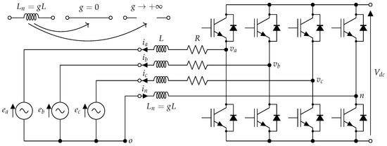
Figure 1.
Grid-connected three-phase, four-wire, four-leg inverter.
Similarly to the conventional three-phase inverter, it is possible to employ advanced PWM schemes (often referred to as PWM common-mode injection) such as SVPWM and DPWM to achieve greater DC-link utilization and switching-loss reduction [14]. The common-mode voltage is directly influenced by the fourth leg and can be driven accordingly to the chosen common-mode injection technique [19]. All the phases present the same coupling inductance L, and all PWM carriers are synchronized at the same switching frequency . The neutral inductor can be either included or not according to design specifications. In the case of the neutral inductor’s absence, phase analysis is particularly straightforward, since the converter can be seen as three single-phase full-bridge inverters sharing a fourth leg [25]. On the other hand, a parameterized neutral inductor, as depicted in Figure 1, permits the study of virtually infinite intermediate configurations ranging from the conventional three-phase inverter to a four-leg inverter without a neutral inductor [13].
The converter acts as an active rectifier when the power flow is directed from AC to DC. On other hand, when power flow is directed from DC to AC, the converter acts effectively as an inverter. The latter operation is particularly useful in transportation electrification (vehicle-to-grid and vehicle-to-vehicle) and grid integration (renewable energy sources and static energy storage) [6,30]. By unbalancing power absorption, it is possible to enable ancillary services such as vehicle-to-grid, -home, and -load; and to ensure compliance with regulatory frameworks such as IEC/TR 61000-3-13 [31,32]. As will be clear later, current ripple is power-flow-direction-invariant; therefore, from now on, the words “inverter”, “rectifier”, and “converter” are freely interchanged, given that developments are valid in all the scenarios regardless of power flow direction.
2.1. Carrier-Based Pulse Width Modulation Principle
In the current subsection, all the statements explicitly refer to the so-called carrier-based approach. In its simplest realization, three modulating signals are compared with a triangular carrier (usually ranging the span ) to achieve desired PWM pattern. Each modulating signal is simply the reference AC voltage that the inverter has to generate scaled by the DC-link voltage . It has been demonstrated that a one-to-one link between carrier-based and space-vector modulations always exists; therefore, all the findings discussed in this manuscript do not suffer from any loss of generalization [15,21].
Thanks to the peculiarity of having the neutral wire connected to a dedicated fourth leg, it is possible to control the middle point voltage at will. Indeed, this fact is at the basis of the common-mode injection. Modulating signals (neutral included) are characterized by a certain common-mode as:
having , a sinusoidal reference signal; m, modulation index; and , phase angle. The place holder x represents any of the phases (a, b, and c), and the neutral phase is n. In the current manuscript, the modulation index is defined as:
where V is the mains’ voltage’s RMS. Multiple literature contributions used as normalization base effectively double modulation index span; e.g., m = M/2 in [14]. This manuscript focused on grid-connected applications. Each phase modulation index was assumed to be similar, even in the case of unbalanced operations.
2.2. Most Popular Common-Mode Injections
The so-called SPWM represents the most basic modulation scheme because of its continuously null common-mode injection. Due to an m limited in the range , no DC-link utilization improvement can be achieved.
On the other hand, the space vector’s most straightforward modulation is the so-called SVM, which evenly distributes zero-configuration (000 and 111) across one switching cycle. Modulation range is extended up to , leading to DC-link utilization; being the biggest radius on the hexagon [33]. The related carrier-based implementation is known as SVPWM, and it can be realized through the not trivial injection:
which affectedly obtains a perfect centering of the modulating signals across the triangle carrier span. It is indeed also known as centered PWM (CPWM).
Historically, particular interest has been devoted to the THIPWM class of techniques. The common-mode injection consists of a third-harmonic signal that in the most popular implementation could have amplitude or in the case of THIPWM/6 or THIPWM/4, respectively. THIPWM/6 can reach a modulation index up to , and THIPWM/4 is limited to , ensuring only a increment in the DC-link utilization. In spite of the simple definition, the realization of a synchronized harmonic at three times the switching frequency has not been proven trivial, and quickly academic and industrial interest shifted toward more rewarding SVPWM/CPWM [14,19].
The DPWM class of injections represents perhaps the most interesting family of techniques. Although it always ensures the extension of the modulation index up to , it presents the interesting feature of suppressing of the commutations of each phase in every fundamental period. The latter feature is obtained by alternatively clamping modulation signals towards carrier upper () and lower () boundaries. Clearly, reducing switching losses is the primary outcome enabled by this modulation family. Most straightforward implementations of DPWM are DPWMMAX and DPWMMIN techniques, which clamp modulating signals at the upper or lower modulation limit, respectively; this is equivalent to utilizing only the space vector zero-configuration 111, or 000 [15,19]. DPWMMAX is obtained by utilizing:
and DPWMMIN is realized with:
A direct evolution of DPWM consists of the so-called generalized DPWM (GDPWM), whose main feature consists of the distribution of two clamping windows according to current maximum absolute value; clamping instants are strongly dependent on voltage and current phase angle , and therefore, power factor (PF). Most popular GDPWM injections are DPWM0, DPWM1, and DPWM2, obtained with , , and , respectively. DPWM1 is therefore particularly effective when the PF is close to unity, and therefore, it is by far the most popular one. The last DPWM injection that can be inserted in the GDPWM umbrella is the so-called DPWM3. Differently from the others, each phase presents four clamping windows located in such a way as to ensure commutation interdiction when the current is at its peak and the power factor is around zero. Indeed, it is particularly effective when the reactive power control is the main target (STATCOM-like behavior). Every DPWM clamping action is obtained by alternating DPWMMAX and DPWMMIN common-mode injections given in Equations (4) and (5).
A broad description of each PWM modulation together with carrier-based implementation details is available in [14,15,19]. The main features of each common-mode injection are collected in Table 1.

Table 1.
Popular PWM common-mode injections and their main features.
3. Current Ripple Generalization
Each phase voltage, (difference between x-th pole voltage and the voltage at the common point o), presents a pulsed waveform that can be split in AC component (base-band at the mains frequency) and a ripple contribution (arranged in clusters at multiples) as .
Phase current flow is caused by the voltage drop across the coupling impedance L, whose internal series resistance is indicated as R. Each phase equation can be described as:
with being the x-th phase’s mains voltage. Since this manuscript’s scope deals with switching current ripple only (supra harmonics), grid voltages are considered perfectly sinusoidal, and no low-frequency distorted component is considered.
Due to the above considerations, an AC current contribution caused by the instantaneous difference between and and responsible for the active and reactive power exchanged can be defined. Additionally, a current ripple component solely caused by the high-frequency voltage can be defined as:
which yields (neglecting voltage drop on R):
with if the initial time instant is considered at current ripple zero-crossing; from now on, the term is omitted for the sake of simplicity. The current ripple is PF-invariant, and therefore, power-flow-orientation-invariant.
From Figure 1 it is possible to determine high-frequency voltage across inductors L as:
where (difference between voltage at the common point o and neutral pole voltage) can be determined by employing Millman’s theorem as:
having a difference between the x-th phase and neutral pole voltages, virtual neutral voltage, and g neutral inductor parametric factor ( as defined in [13]). As is foreseeable, in the case of a neutral wire straight connection, leads to . On the other hand, in the case of conventional three-phase inverter (), Equation (10) reverts to the simple average of pole voltages.
Equation (10) can be effectively employed in the determination of neutral current ripple in a similar fashion, as done above. Indeed integrating , neutral current ripple is expressed as:
3.1. Current Ripple in the case of a Neutral Straight Connection
As anticipated above, in the case of neutral straight connection parameter, . This presents the immediate consequence of amending Equation (8) as:
highlighting that each phase’s current ripple is independent of the others.
Equation (11) is updated as:
showcasing the trivial result that the neutral current ripple is the direct summation of phase current ripples.
Time-domain analysis of phase and neutral current ripple envelopes, maximum peak-to-peak, and RMS in case of all the common-mode injections of Table 1 is available in [19,25] for the case of . Such an in-depth analysis has been possible thanks to the above-pointed-out phase independence that permits one to study of each current ripple on its own. Among the various results, it is possible to recall that:
- SVPWM, THIPWM/4, and THIPWM/6 present similar behaviors in terms of maximum value and RMS;
- DPWMMAX, DPWMMIN, DPWM0, and DPWM2 present always-coinciding maximum values and RMS;
- Neutral current ripple is common-mode injection-independent.
Being the main focus of this manuscript, the generalized description of phase and neutral-current-ripple RMS, Table 2, collects all RMS formulations available from [19].
Table 2.
Phase and neutral-current-ripple RMS in the case of and .
3.2. Current Ripple Time-Domain Generalization
By replacing Equations (9), (10), (12) and (13) inside Equation (8), it is possible to reach the phase current ripple’s not-trivial generalized relationships:
On the other hand, by replacing Equation (13) in Equation (11), generalized neutral current ripple becomes:
preserving common-mode injection independence.
Equations (14) and (15) state that phase current ripples in case of a generic neutral inductor are made out of the phase current ripple that would flow without the neutral inductor () subtracted of the neutral current ripple that would flow without the neutral inductor () scaled by the factor . Additionally, the neutral current ripple is directly the neutral current ripple that would flow without the neutral inductor () scaled by the factor . This generalization represents in a not-obvious result, and it provides a powerful tool for having a complete understanding of harmonic pollution in grid-connected three-phase inverters. Indeed, setting , Equations (14) and (15) revert to the trivial case while . On the other hand, it is also possible to define the phase current ripple in conventional three-leg inverters (which do not have a neutral wire, i.e., ) by means of the counterintuitive relationship:
3.3. Generalized Phase-Current-Ripple RMS Close-Form Derivation
From Equation (14), the phase-current-ripple RMS can be computed as:
whose integral term can be rewritten as:
showing that its result is common-mode injection-invariant because it is derived from neutral-current-ripple RMS that is injection-invariant itself. Indeed, as a counter-check, deriving the integral term inside Equation (17) from any of the known cases of Table 2 (see ) is:
and it always leads to:
Therefore, generalized phase-current-ripple RMS becomes:
which can be rewritten in the compact form:
where
having as the sole injection-dependent term; it should be replaced with any of the formulations shown in Table 2 (see ). Interestingly, Equation (22) can be employed with any arbitrary PWM scheme as long as its behavior in terms of , and is known at . Clearly, characterizing the VSI for automatically extended the results over any arbitrary value of neutral inductance .
Term quickly tends to the asymptotic value , showing , , , and convergence already for , , , and , respectively; this result is in strong agreement with what is shown in [13] for the sole SPWM injection. Small values of neutral inductors lead the four-leg inverter to approach the theoretical optimum () behavior exhibited by standard three-leg inverter [27,28]. Figure 2, Figure 3, Figure 4 and Figure 5 validate general formulation (22) for all the common-mode injections listed in Table 1 in the cases of , , , and , respectively (i.e., , , , and ). As is clearly visible in Figure 5, neutral inductor almost perfectly retraces conventional three-phase inverter behavior (indicated as “3-leg”) due to its convergence discussed above; similar considerations are visible in Figure 4 in the case of . Additionally, for low values of the modulation index (roughly ), harmonic pollution levels are roughly the same regardless of the value of g. In all the cases, numerical data points fairly match predicted trending over the whole m diapason for all the tested values of neutral inductance. Numerical validations were performed using PLECS (Plexim) on the same setup discussed in [13,19]. Symbol indicates normalized formulations; normalization base .
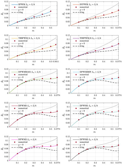
Figure 2.
Numerical validation of normalized phase-current-ripple RMS in the case of multiple PWM common-mode injections for (i.e., ). Normalization base .
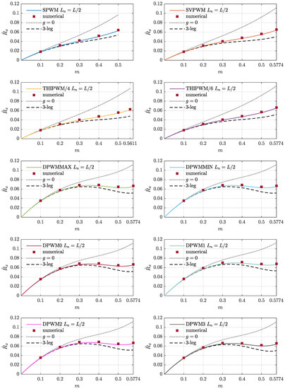
Figure 3.
Numerical validation of normalized phase-current-ripple RMS in the case of multiple PWM common-mode injections for (i.e., ). Normalization base .
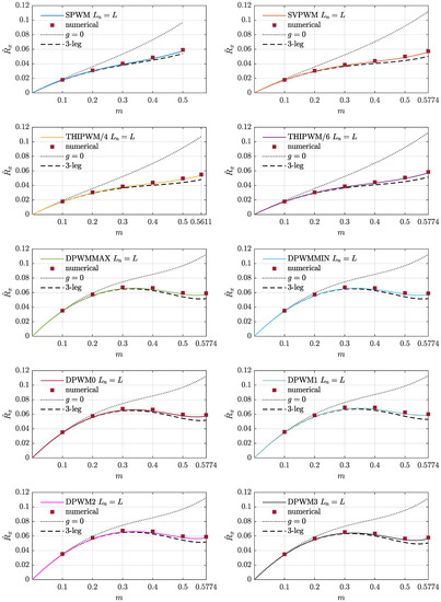
Figure 4.
Numerical validation of normalized phase-current-ripple RMS in the case of multiple PWM common-mode injections for (i.e., ). Normalization base .
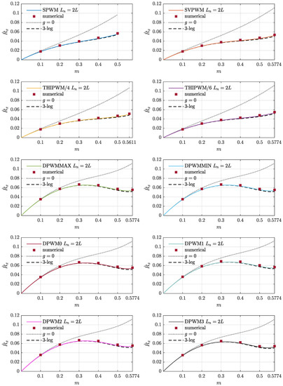
Figure 5.
Numerical validation of normalized phase-current-ripple RMS in the case of multiple PWM common-mode injections for (i.e., ). Normalization base .
3.4. Generalized Neutral-Current-Ripple RMS Closed-Form Derivation
Generalized neutral-current-ripple RMS is derived from (15) as:
which has been validated in Figure 6 in the cases of , , , and . The more-than-hyperbolic trend permits harmonic pollution reductions of 43%, 60%, 75%, and 86% with respect to the four-leg inverter with a straight neutral connection () in the cases of , , , and , respectively. Additionally, in this case symbol, indicates normalized results. In all the cases, numerical data points fairly match predicted trending over the whole m diapason for all the tested values of the neutral inductor. As anticipated, neutral current ripple is common-mode injection-invariant.
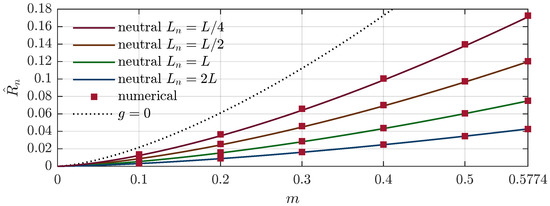
Figure 6.
Numerical validation of normalized neutral-current-ripple RMS for , , , and (i.e., , , , and ). Normalization base .
4. Experimental Validation
This section reports the experimental validation results obtained by the laboratory test bench displayed in Figure 7. Table 3 collects setup main parameters; the experimental setup was identical to the numerical one.
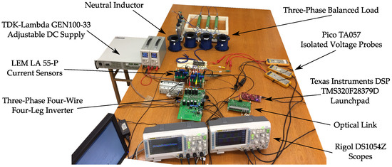
Figure 7.
View of the laboratory test bench together with the devices used for control and acquisition.
Table 3.
Experimental setup’s main system parameters.
4.1. Description of the Experimental Test Bench
The experimental test bench consisted of a unity power-factor three-phase load connected to the four-wire four-leg inverter, as depicted in Figure 8. Each inductor had an air core to preserve linearity at all current levels. On the other hand, each power resistor’s thermal stability was ensured by forced-air cooling. Every measurement was performed by alternating settling and idle times of 10 and 90 s each, respectively. This configuration was characterized by DC to AC power flow and can be run without the need for any closed-loop control. The three-phase four-leg inverter was made out using four legs of two three-phase IGBT power module, PS22A76 (Mitsubishi Electric), and it was fed by a GEN100-33 (TDK-Lambda) controllable power supply. The inverter was driven using a TMS320F28379D Launchpad (Texas Instruments) DSP whose code was deployed directly from MATLAB/Simulink (Mathworks) environment. Currents were sensed using LA 55-P (LEM) current transducer operated at ambient temperature, with a supply voltage of V and a 100 SMD shunt resistor. Data were acquired by employing DS1054Z (Rigol Technologies) digital oscilloscopes using a 5 MS/s sampling rate.
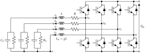
Figure 8.
Three-phase, four-wire, four-leg inverter with a parametric neutral inductor.
The experimental setup was iterated three times considering , , and . Neutral inductor values were obtained by series/parallel combinations of inductors nominally equal to the one used on the phases. In this way, ratios of about , , and were obtained. Figure 7 shows the setup corresponding with (i.e., ).
4.2. Discussion of the Experimental Results
To verify the actual validity of the proposed generalized RMS formulations, several experimental results were acquired. Similarly to what was performed in the numerical validation, modulation index m diapason was spanned with steps of 0.1 for the final value, which could be either 0.5 or depending on the type of modulation scheme. Nonidealities (e.g., dead time, noise, transducer accuracy, and cabling parasitic inductance and resistance) were not compensated during data post-processing. Modulation schemes SPWM, SVPWM, and DPWM1 were selected by virtue of their industrial relevance.
4.2.1. Phase-Current-Ripple RMS
Figure 9 shows the experimental validation of the normalized phase current ripple generalized RMS formulation in the case of SPWM. Each frame shows , , and (from left to right). As is visible, the predicted trending was confirmed over the whole modulation index range and for all the values of neutral inductance. Table 4 reports experimental data , theoretical value , and the corresponding relative error in percentage . As was foreseeable, low-power values (i.e., ) are more influenced by the experimental noise. Indeed, the relative error is roughly double all the other ones—in all the cases well below 10%. Overall, the same values of m presented comparable uncertainty, showing that experimental condition stability was ensured throughout the whole testing duration.
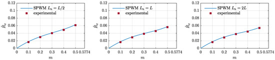
Figure 9.
Experimental validation of normalized phase-current-ripple RMS in the case of SPWM for , , and (i.e., , , and ). Normalization base .
Table 4.
Phase-current-ripple RMS experimental errors assessment in the case of SPWM for , , and (i.e., , , and ).
Experimental results related to SVPWM are reported in Figure 10 and Table 5 following the same approach introduced above. Additionally, in this case the general trend is validated for all the values of modulation index and neutral inductance. Again, the highest errors are for low power values (well below 10%), attesting to experimental noise’s influence.
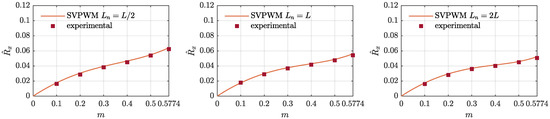
Figure 10.
Experimental validation of normalized phase-current-ripple RMS in the case of SVPWM for , , and (i.e., , , and ). Normalization base .
Table 5.
Phase-current-ripple RMS experimental errors assessment in the case of SVPWM for , , and (i.e., , , and ).
Finally, validation concerning DPWM1 technique is given in Figure 11 and Table 6. The above considerations retain validity also under DPWM1 without any noticeable exception.
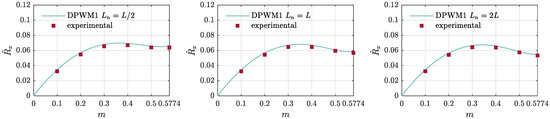
Figure 11.
Experimental validation of normalized phase-current-ripple RMS in the case of DPWM1 for , , and (i.e., , , and ). Normalization base .
Table 6.
Phase-current-ripple RMS experimental errors assessment in the case of DPWM1 for , , and (i.e., , , and ).
The overall predicted trending is validated with a fairly good matching regardless of modulation index m, neutral inductor , and PWM scheme. This overall behavior corroborates the proposed generalized RMS formulation consistency.
4.2.2. Neutral-Current-Ripple RMS
Figure 12 shows several experimental validations of the normalized neutral current ripple-generalized RMS as a function of the modulation index m for , , and (i.e., , , and ); normalization base . The overall predicted trending was validated with a fairly good matching of experimental data points for all the considered values of neutral inductor. The latter statement is quantitatively confirmed in Table 7, where experimental data , theoretical value , and the corresponding relative error in percentage are reported. Due to the shallow value of neutral-current-ripple RMS in the case of , the relative error is higher than in the other cases. Despite experimental setup nonidealities, the normalized neutral current ripple-generalized RMS formulation was consistently validated with fairly s,a;; error values.
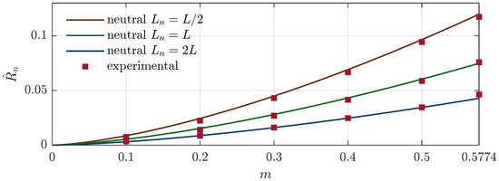
Figure 12.
Experimental validation of normalized neutral-current-ripple RMS for , , and (i.e., , , and ). Normalization base .
Table 7.
Neutral-current-ripple RMS experimental error assessment for , , and (i.e., , , and ).
5. Conclusions
This manuscript proposed closed-form generalizations of the phase and neutral-current-ripple RMS formulations for any kind of PWM scheme for a three-phase, four-leg inverter with a neutral inductor. The proposed approach employs a parametric description of the neutral inductor in relation to the phase ones. This generalization permits precise calculation of current-ripple RMS bridging from a four-leg inverter with a straight neutral connection (no neutral inductor) to the conventional three-phase inverter (no neutral wire), paving the way for a unique formulation for virtually any four-leg inverter. The formulations have been explicitly shown for the most popular PWM common-mode injections, namely, SPWM, SVPWM, THIPWM, and several DPWMs. Its validity extends to any arbitrary PWM scheme, as long as basic knowledge of phase and neutral-current-ripple RMS is available in the case of a neutral straight connection.
Counterintuitively, even relatively small values of neutral inductors enable noticeable abatement of phase and neutral harmonic pollution. Indeed, neutral inductors equal to 25%, 50%, 100%, and 200% phase ones, respectively, ensure 67%, 84%, 94%, and 98% convergence of the phase current ripple’s harmonic performance with respect to the conventional three-phase inverter. On the other hand, the same values of inductance ensure more-than-hyperbolic neutral-current-ripple RMS reductions of 43%, 60%, 75%, and 86% with respect to the four-leg inverter without the neutral inductor. A total of 287 numerical and experimental results extensively validated the proposed formulations in several PWM schemes and neutral inductors.
Future developments could focus on minimizing the total installed inductance in specific scenarios and applications. A comparison between several PWM schemes could enable magnet-size savings and switching-loss reduction.
Author Contributions
Conceptualization, R.M.; methodology, R.M. and F.L.F.; software, R.M. and F.L.F.; validation, R.M., M.R. and G.G.; formal analysis, R.M. and F.L.F.; investigation, R.M.; resources, M.R. and G.G.; data curation, R.M. and F.L.F.; writing—original draft preparation, R.M., F.L.F., M.R. and G.G.; writing—review and editing, R.M., F.L.F., M.R. and G.G.; visualization, R.M.; supervision, M.R. and G.G. All authors have read and agreed to the published version of the manuscript.
Funding
This research received no external funding.
Data Availability Statement
Not applicable.
Conflicts of Interest
The authors declare no conflict of interest.
References
- Zhong, Q.C. Power-electronics-enabled autonomous power systems: Architecture and technical routes. IEEE Trans. Ind. Electron. 2017, 64, 5907–5918. [Google Scholar] [CrossRef]
- Meinguet, F.; Semail, E.; Gyselinck, J. Enhanced control of a PMSM supplied by a four-leg voltage source inverter using the homopolar torque. In Proceedings of the 2008 18th International Conference on Electrical Machines, Vilamoura, Portugal, 6–9 September 2008; pp. 1–6. [Google Scholar]
- Vechiu, I.; Camblong, H.; Tapia, G.; Dakyo, B.; Curea, O. Control of four leg inverter for hybrid power system applications with unbalanced load. Energy Convers. Manag. 2007, 48, 2119–2128. [Google Scholar] [CrossRef]
- Dong, G.; Ojo, O. Current regulation in four-leg voltage-source converters. IEEE Trans. Ind. Electron. 2007, 54, 2095–2105. [Google Scholar] [CrossRef]
- Yilmaz, M.; Krein, P.T. Review of battery charger topologies, charging power levels, and infrastructure for plug-in electric and hybrid vehicles. IEEE Trans. Power Electron. 2012, 28, 2151–2169. [Google Scholar] [CrossRef]
- Lo Franco, F.; Mandrioli, R.; Ricco, M.; Monteiro, V.; Monteiro, L.F.; Afonso, J.L.; Grandi, G. Electric Vehicles Charging Management System for Optimal Exploitation of Photovoltaic Energy Sources Considering Vehicle-to-Vehicle Mode. Front. Energy Res. 2021, 9, 716389. [Google Scholar] [CrossRef]
- Rafi, F.H.M.; Hossain, M.; Rahman, M.S.; Taghizadeh, S. An overview of unbalance compensation techniques using power electronic converters for active distribution systems with renewable generation. Renew. Sustain. Energy Rev. 2020, 125, 109812. [Google Scholar] [CrossRef]
- Mandrioli, R.; Viatkin, A.; Hammami, M.; Ricco, M.; Grandi, G. Variable switching frequency PWM for three-phase four-wire split-capacitor inverter performance enhancement. IEEE Trans. Power Electron. 2021, 36, 13674–13685. [Google Scholar] [CrossRef]
- Nascimento, C.F.; Diene, O.; Watanabe, E.H. Analytical model of three-phase four-wire VSC operating as grid forming power converter under unbalanced load conditions. In Proceedings of the 2017 IEEE 12th International Conference on Power Electronics and Drive Systems (PEDS), Honolulu, HI, USA, 12–15 December 2017; pp. 1–219. [Google Scholar]
- Mandrioli, R.; Ricco, M.; Grandi, G.; Pereira, T.A.; Liserre, M. DAB-Based Common-Mode Injection in Three-Phase Four-Wire Inverters. In Proceedings of the 2022 IEEE 16th International Conference on Compatibility, Power Electronics, and Power Engineering (CPE-POWERENG), Birmingham, UK, 29 June–1 July 2022; pp. 1–6. [Google Scholar]
- Hintz, A.; Prasanna, U.R.; Rajashekara, K. Comparative study of the three-phase grid-connected inverter sharing unbalanced three-phase and/or single-phase systems. IEEE Trans. Ind. Appl. 2016, 52, 5156–5164. [Google Scholar] [CrossRef]
- Lin, Z.; Ruan, X.; Jia, L.; Zhao, W.; Liu, H.; Rao, P. Optimized design of the neutral inductor and filter inductors in three-phase four-wire inverter with split DC-link capacitors. IEEE Trans. Power Electron. 2018, 34, 247–262. [Google Scholar] [CrossRef]
- Viatkin, A.; Mandrioli, R.; Hammami, M.; Ricco, M.; Grandi, G. AC Current Ripple in Three-Phase Four-Leg PWM Converters with Neutral Line Inductor. Energies 2021, 14, 1430. [Google Scholar] [CrossRef]
- Holmes, D.G.; Lipo, T.A. Pulse Width Modulation for Power Converters: Principles and Practice, 1st ed.; Wiley-IEEE Press: Hoboken, NJ, USA, 2003. [Google Scholar]
- Hava, A.M.; Kerkman, R.J.; Lipo, T.A. Simple analytical and graphical methods for carrier-based PWM-VSI drives. IEEE Trans. Power Electron. 1999, 14, 49–61. [Google Scholar] [CrossRef]
- Hava, A.M.; Kerkman, R.J.; Lipo, T.A. Carrier-based PWM-VSI overmodulation strategies: Analysis, comparison, and design. IEEE Trans. Power Electron. 1998, 13, 674–689. [Google Scholar] [CrossRef]
- Llonch-Masachs, M.; Heredero-Peris, D.; Montesinos-Miracle, D.; Rull-Duran, J. Understanding the three and four-leg inverter Space Vector. In Proceedings of the 2016 18th European Conference on Power Electronics and Applications (EPE’16 ECCE Europe), Karlsruhe, Germany, 5–9 September 2016; pp. 1–10. [Google Scholar]
- Heredero-Peris, D.; Llonch-Masachs, M.; Chillón-Antón, C.; Bergas-Jané, J.G.; Pagès-Giménez, M.; Sumper, A.; Montesinos-Miracle, D. Extending 2-D space vector PWM for three-phase four-leg inverters. EPE J. 2019, 29, 132–148. [Google Scholar] [CrossRef]
- Mandrioli, R.; Viatkin, A.; Hammami, M.; Ricco, M.; Grandi, G. A comprehensive AC current ripple analysis and performance enhancement via discontinuous PWM in three-phase four-leg grid-connected inverters. Energies 2020, 13, 4352. [Google Scholar] [CrossRef]
- Zhang, R.; Prasad, V.H.; Boroyevich, D.; Lee, F.C. Three-dimensional space vector modulation for four-leg voltage-source converters. IEEE Trans. Power Electron. 2002, 17, 314–326. [Google Scholar] [CrossRef]
- Zhou, K.; Wang, D. Relationship between space-vector modulation and three-phase carrier-based PWM: A comprehensive analysis [three-phase inverters]. IEEE Trans. Ind. Electron. 2002, 49, 186–196. [Google Scholar] [CrossRef]
- Jadeja, R.; Ved, A.D.; Chauhan, S.K.; Trivedi, T. A random carrier frequency PWM technique with a narrowband for a grid-connected solar inverter. Electr. Eng. 2020, 102, 1755–1767. [Google Scholar] [CrossRef]
- Jiang, D.; Wang, F. Current-ripple prediction for three-phase PWM converters. IEEE Trans. Ind. Appl. 2013, 50, 531–538. [Google Scholar] [CrossRef]
- Zijiang, W.; Qionglin, L.; Yuzheng, T.; Shuming, L.; Shuangyin, D. Comparison of harmonic limits and evaluation of the international standards. MATEC Web Conf. 2019, 277, 03009. [Google Scholar]
- Viatkin, A.; Mandrioli, R.; Hammami, M.; Ricco, M.; Grandi, G. AC Current Ripple Harmonic Pollution in Three-Phase Four-Leg Active Front-End AC/DC Converter for On-Board EV Chargers. Electronics 2021, 10, 116. [Google Scholar] [CrossRef]
- Cai, W.; Shen, Y.; Xiao, X.; Wang, W.; Zhang, W.; Li, K.; Zhang, C.; Zhao, Z. Design of the Neutral Line Inductor for Three-phase Four-leg Inverters. In Proceedings of the 2019 IEEE Sustainable Power and Energy Conference (iSPEC), Beijing, China, 21–23 November 2019; pp. 2455–2460. [Google Scholar]
- Jahns, T.M.; De Doncker, R.W.; Radun, A.V.; Szczesny, P.M.; Turnbull, F.G. System design considerations for a high-power aerospace resonant link converter. IEEE Trans. Power Electron. 1993, 8, 663–672. [Google Scholar] [CrossRef]
- Liu, Z.; Liu, J.; Li, J. Modeling, analysis, and mitigation of load neutral point voltage for three-phase four-leg inverter. IEEE Trans. Ind. Electron. 2012, 60, 2010–2021. [Google Scholar] [CrossRef]
- Arif, S.M.; Lie, T.T.; Seet, B.C.; Ayyadi, S.; Jensen, K. Review of electric vehicle technologies, charging methods, standards and optimization techniques. Electronics 2021, 10, 1910. [Google Scholar] [CrossRef]
- Fu, Y.; Li, Y.; Huang, Y.; Lu, X.; Zou, K.; Chen, C.; Bai, H. Imbalanced load regulation based on virtual resistance of a three-phase four-wire inverter for EV vehicle-to-home applications. IEEE Trans. Transp. Electrif. 2018, 5, 162–173. [Google Scholar] [CrossRef]
- Jayatunga, U.; Perera, S.; Ciufo, P.; Agalgaonkar, A. A review of recent investigations on voltage unbalance management: Further contributions to improvement of IEC/TR 61000-3-13: 2008. In Proceedings of the 2014 16th International Conference on Harmonics and Quality of Power (ICHQP), Bucharest, Romania, 25–28 May 2014; pp. 268–272. [Google Scholar]
- Faraji, H.; Nosratabadi, S.M.; Hemmati, R. AC unbalanced and DC load management in multi-bus residential microgrid integrated with hybrid capacity resources. Energy 2022, 252, 124070. [Google Scholar] [CrossRef]
- O’Rourke, C.J.; Qasim, M.M.; Overlin, M.R.; Kirtley, J.L. A geometric interpretation of reference frames and transformations: dq0, clarke, and park. IEEE Trans. Energy Convers. 2019, 34, 2070–2083. [Google Scholar] [CrossRef]
Disclaimer/Publisher’s Note: The statements, opinions and data contained in all publications are solely those of the individual author(s) and contributor(s) and not of MDPI and/or the editor(s). MDPI and/or the editor(s) disclaim responsibility for any injury to people or property resulting from any ideas, methods, instructions or products referred to in the content. |
© 2023 by the authors. Licensee MDPI, Basel, Switzerland. This article is an open access article distributed under the terms and conditions of the Creative Commons Attribution (CC BY) license (https://creativecommons.org/licenses/by/4.0/).