
Recovering Corrupted Data in Wind Farm Measurements: A Matrix Completion Approach


 and
and 
Abstract
:1. Introduction
1.1. Background and Motivation
1.2. Related Studies
2. Materials and Methods
2.1. Theoretical Approach
2.2. The Matrix Completion Problem
2.3. The Singular Value Thresholding Method
2.4. Data Reduction
2.4.1. Turbine Functioning
- There is a cut–in speed below which the turbine is not activated, hence the generated power is 0 kW;
- Above the cut–in speed, the curve has a cubic trend until reaches a rated speed . Above this value, the power generation is kept constant;
- Finally, the turbine is braked and the power generation stopped when the wind speed is above the cut–off speed .
2.4.2. Data Collection
2.4.3. Classification Criteria
Icing
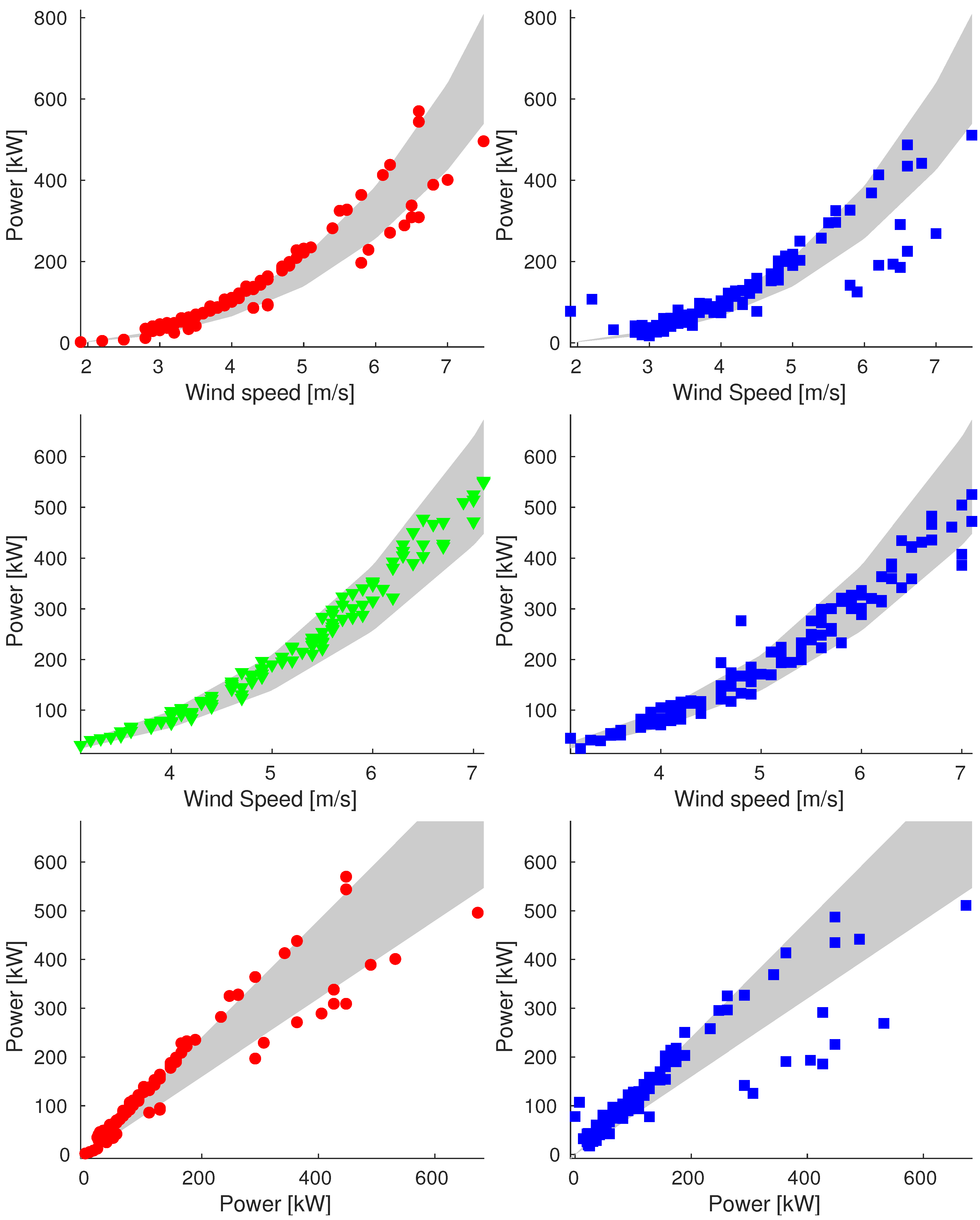
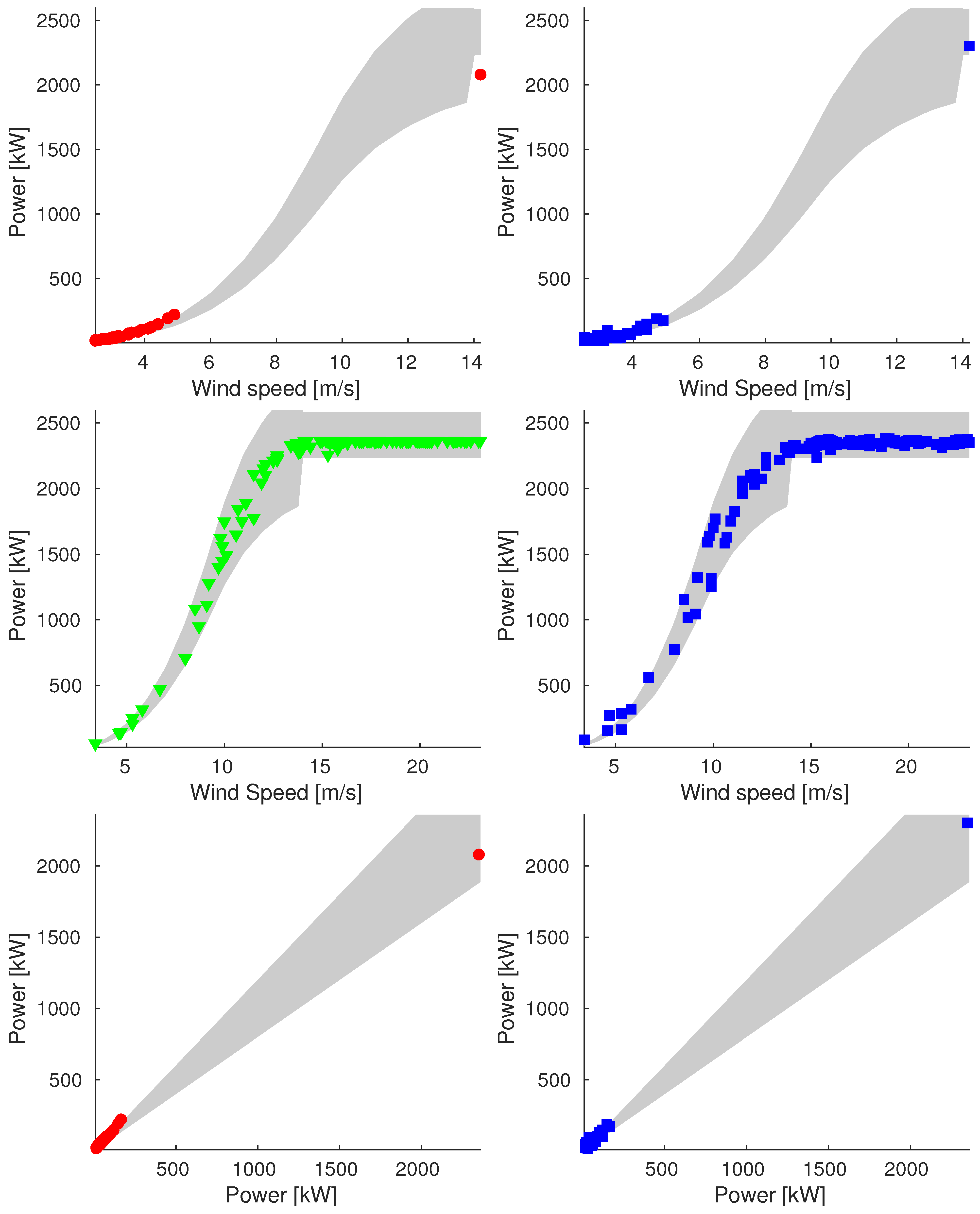
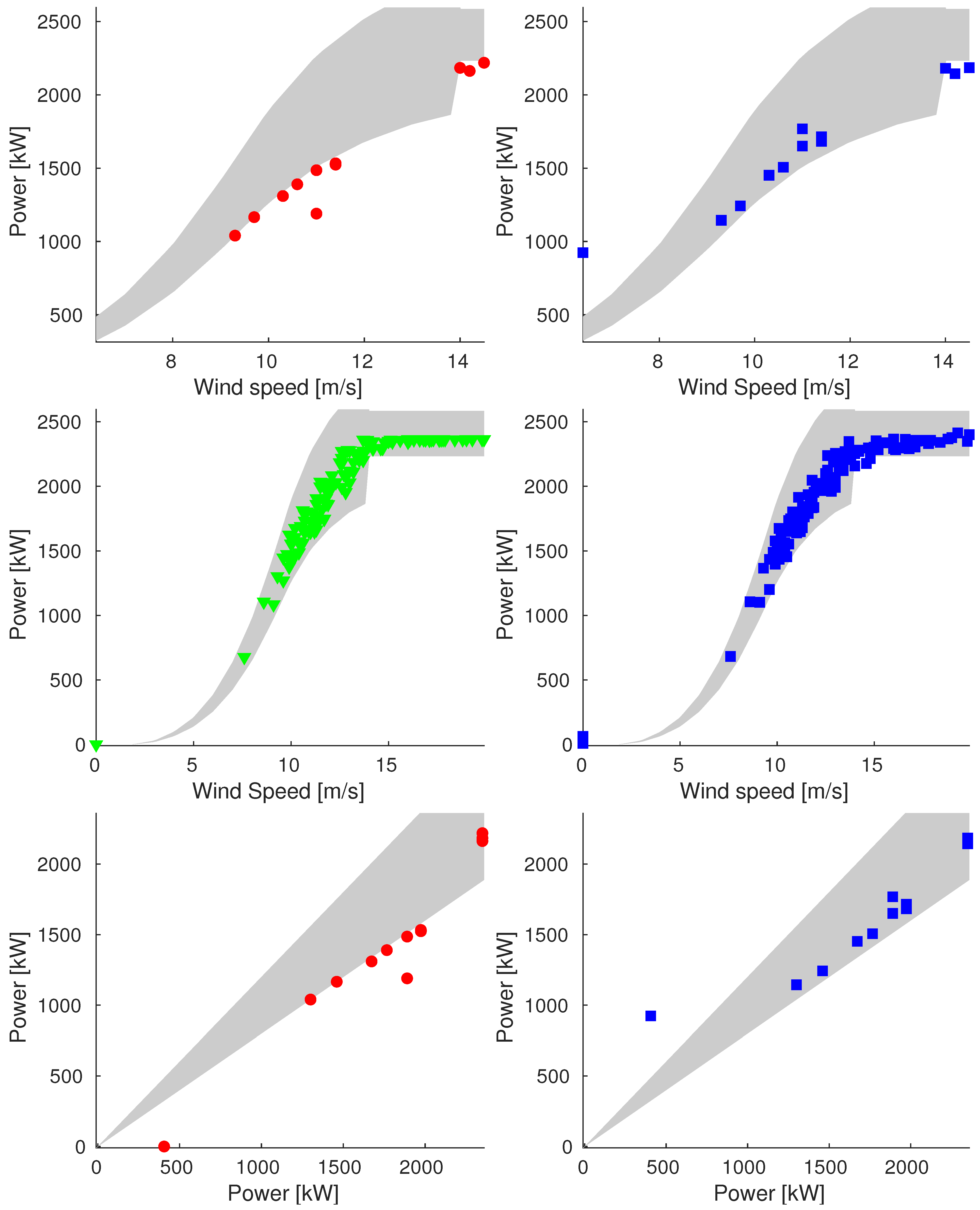
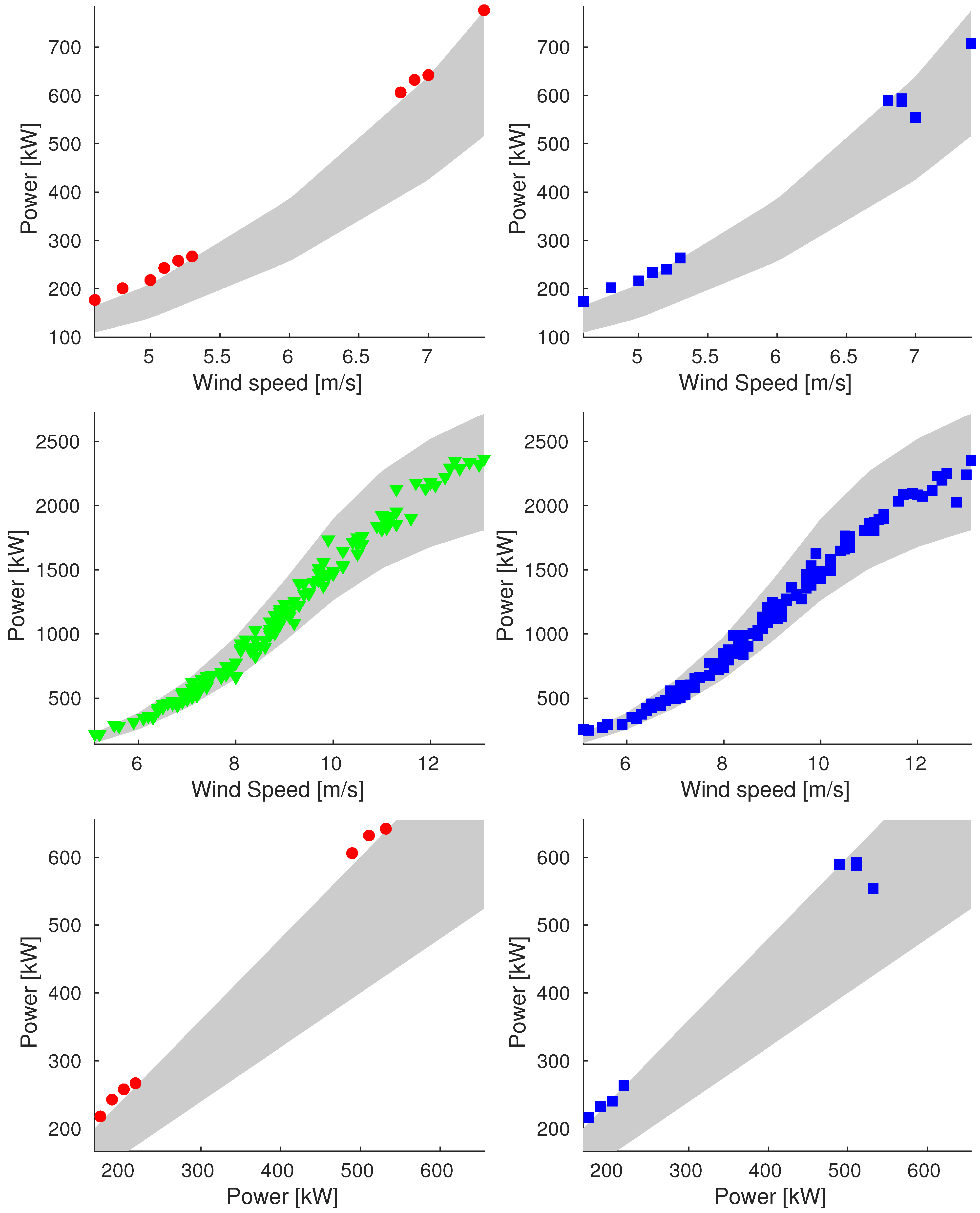
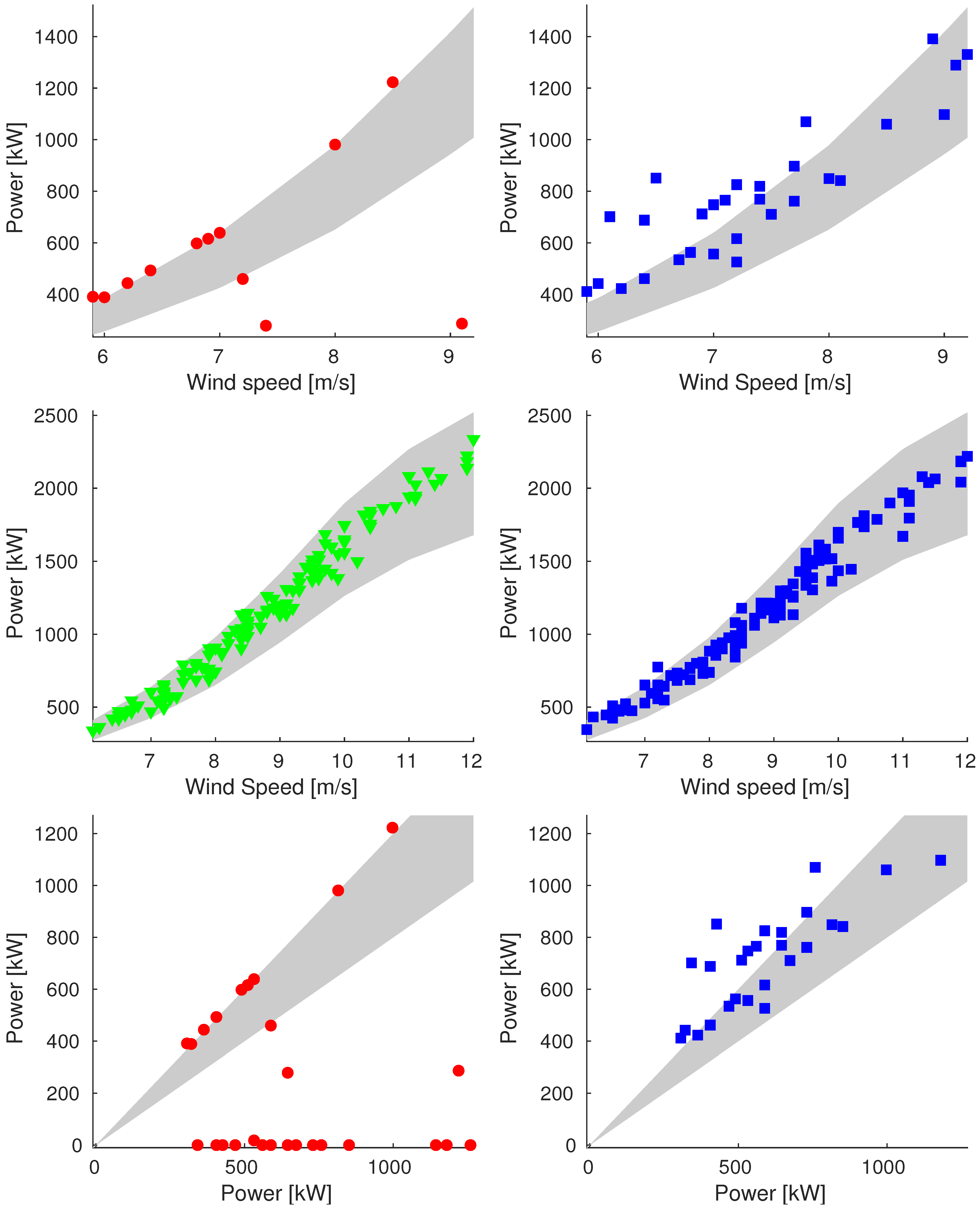
Power Band
- For wind speed values below the cut–in speed , we consider consistent only the data with generated power null, so the band is exactly the power curve;
- For wind speed values included between and , the band is limited by of the theoretical generated power;
- For values included between and , the generated power is kept constant, and the band is limited by +10%/−5% of the theoretical generated power;
- For speed above , the curve is symmetrically extended and the same for the band.
2.5. Recovery Workflow
2.5.1. Building the Data Matrix M
2.5.2. The Training, Validation and Testing Sets
2.5.3. Reconstruction Procedure
- There is at least one interval at which icing occurs. In this case, we have no reliable information for the particular turbine in that timestamp. So, the reconstruction is too hard;
- All the data of one turbine are missing. This can happen due to a blackout or a failure during the whole day.
- After the classification procedure, it happens that the day has less than of consistent timestamps.
3. Results
3.1. Implemented Workflow
- IF there is icing or all data from a turbine are missing: discard the day and skip to Step 3.ELSEClassify the data and build the set .
- IF the data are all consistent, or less than the 50% of data are consistent: discard the day and skip to Step 3.ELSEproceed with recovery:
- (a)
- Rearrange data in matrix M and normalize them to obtain .
- (b)
- Divide consistent data in the training and the validation set. Let be the matrix with 0 entries out of .
- (c)
- Apply the SVT Algorithm 1 with as input matrix. Let be the outcome of the SVT Algorithm.
- (d)
- Denormalize and obtain .
- RETURN
3.2. Summary of Days in 2015
- One day with icing;
- One day with all data missing from a turbine;
- Four days with less than of consistent data;
- Seven days with of consistent data.
- Percentage of consistent data.
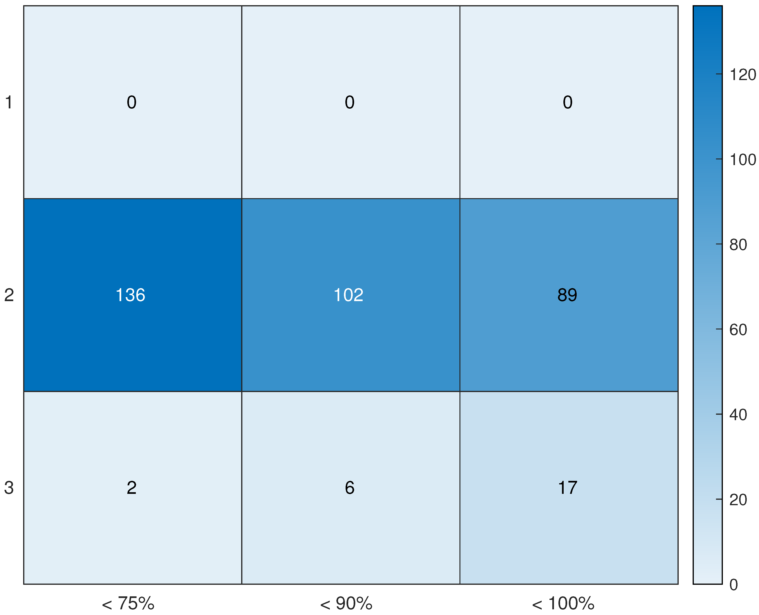
- We consider three groups: Sample_75, days with a percentage of consistent data greater or equal to and less than ; Sample_90, days with a percentage greater or equal to and less than ; Sample_100, days with a percentage greater or equal to .
- Wind speed zone.
- We divide the range of wind speed in three zones: Zone_1 up to ; Zone_2 from to and Zone_3 from on. Then, the days are divided based on in which wind zone the majority of the mean wind speed of inconsistent/missing measurements are.
3.3. Reconstruction Evaluation
- Total Reconstruction Ratei.e., the percentage of reconstructed values of the generated power with respect to all data.
- Relative Reconstruction Ratewhere is the cardinality of the set of rejected timestamps. In other words, is the percentage of reconstructed values of the generated power with respect to the discarded timestamps.
- In order to give more insights on the accuracy of the computed reconstruction, in addition to the total and relative reconstruction rate we provide the value of the following RMSEs:
- -
- RMSE on the training set:
- -
- RMSE on the validation set:
- -
- RMSE of the power data on the testing set:
- -
- RMSE of the power data on the testing set:where is the column index of the theoretical generated power values corresponding to values in the j-th column. (With our arrangement of the data, the theoretical values of generated power are 18 columns ahead of the mean generated power values, i.e., ).
3.4. Numerical Experimentation
| Algorithm 1 SVT Algorithm |
| Input: |
| Output: |
| 1: for to do |
| 2: Compute the SVD of |
| 3: Set |
| 4: if the stopping criterion is satisfied then |
| 5: return |
| 6: end if |
| 7: Set |
| 8: end for |
| 9: return |
4. Discussion
4.1. Comments on Numerical Results
4.2. Conclusions and Perspectives
Author Contributions
Funding
Informed Consent Statement
Data Availability Statement
Acknowledgments
Conflicts of Interest
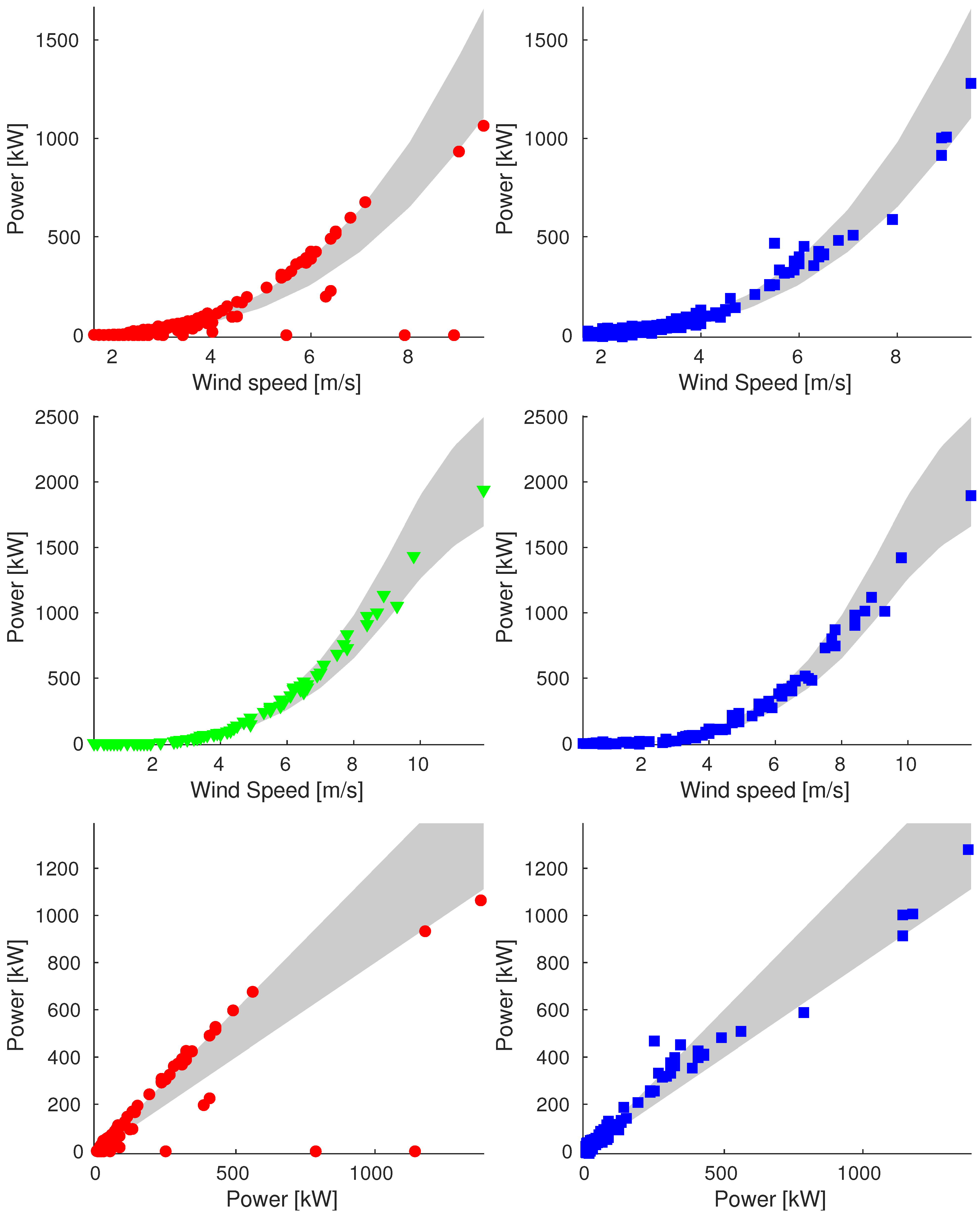
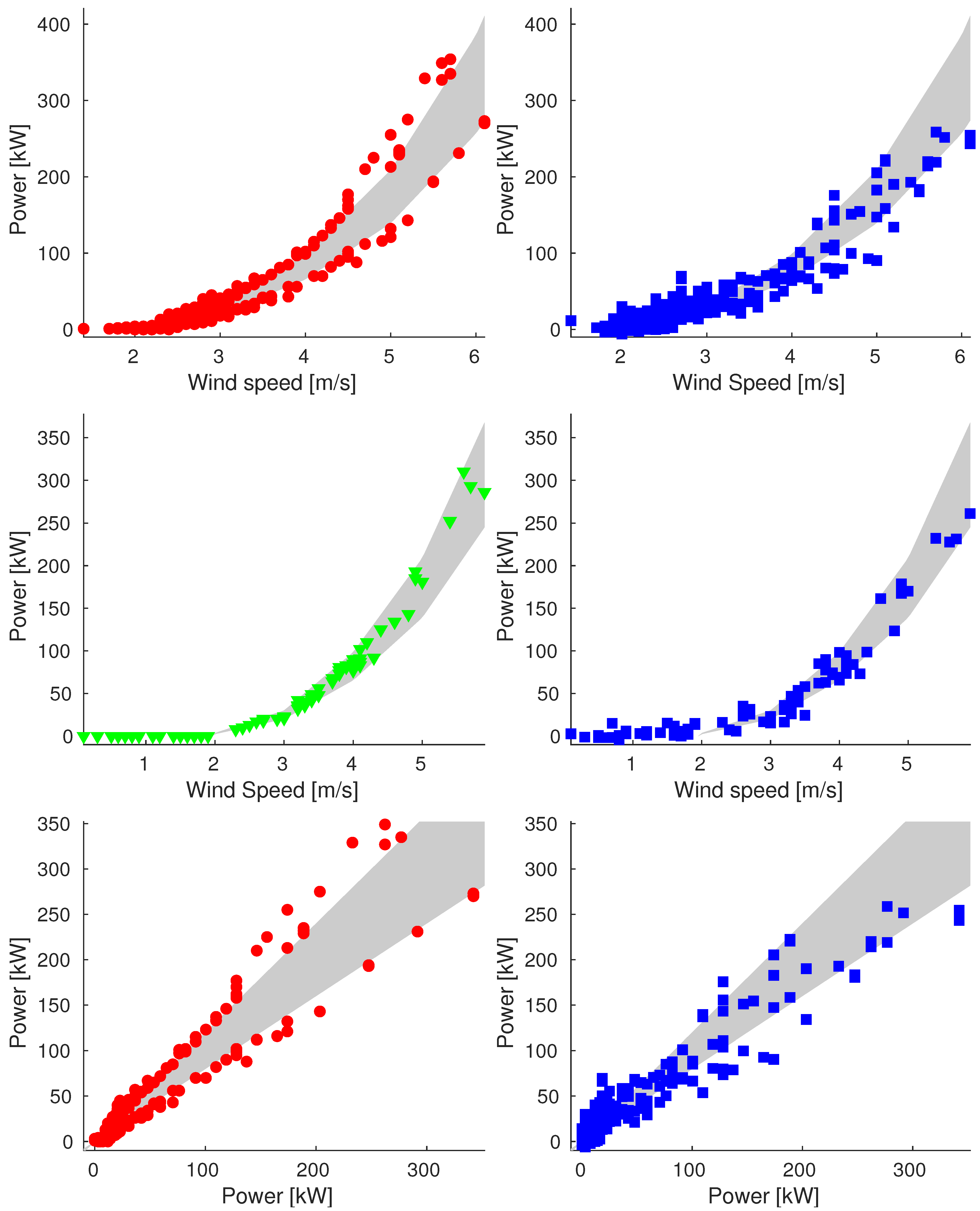
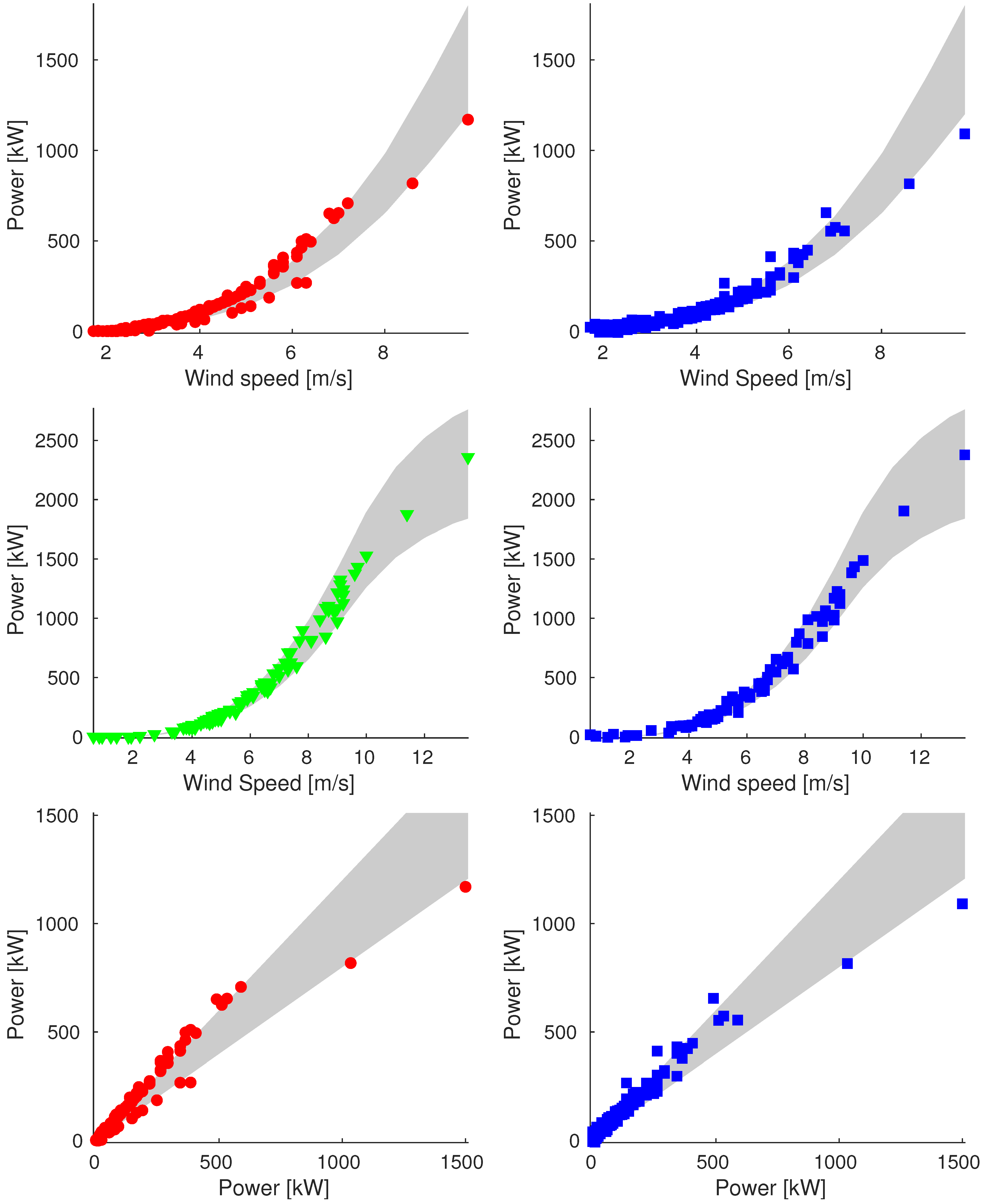
Appendix A. Additional Images
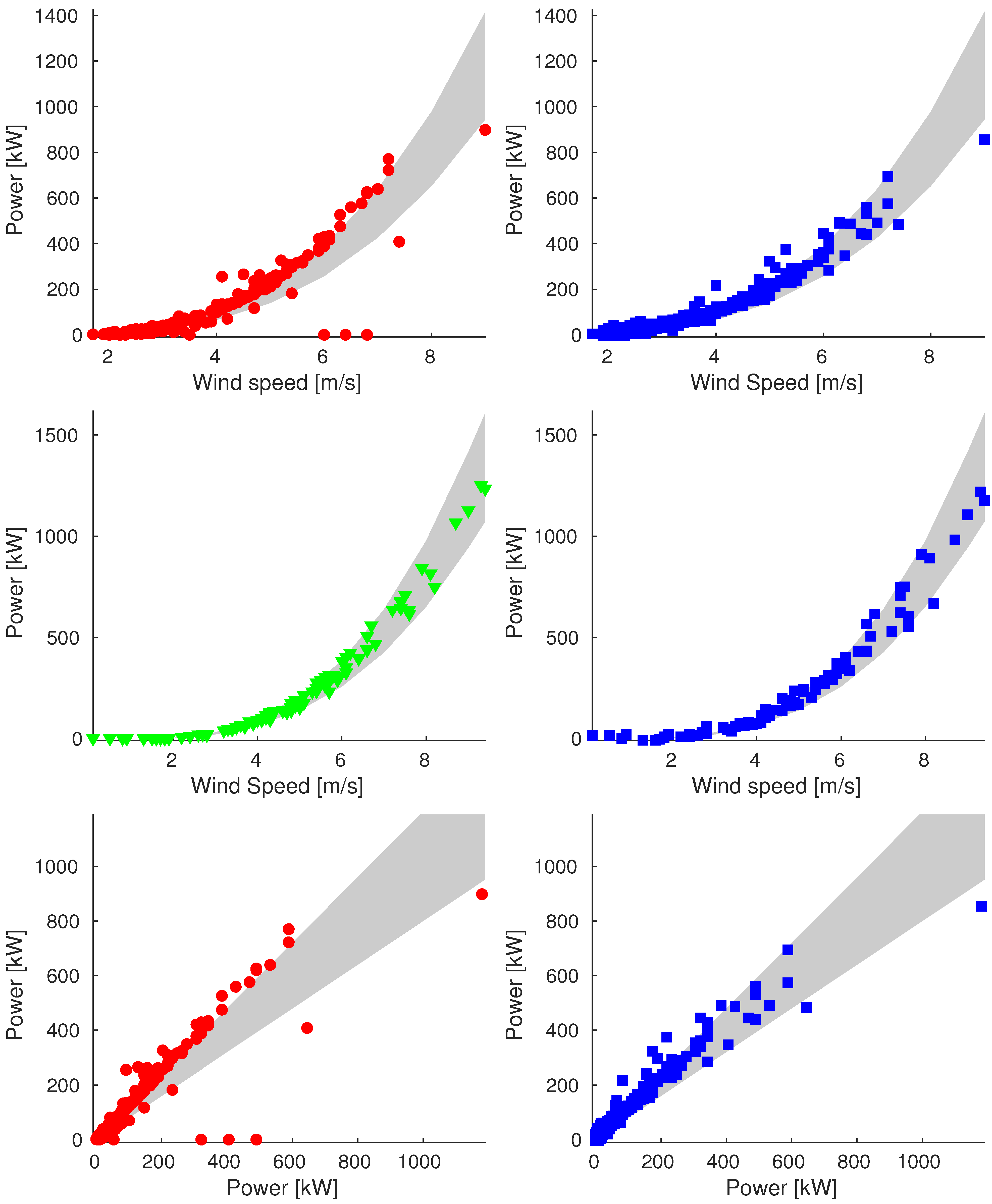
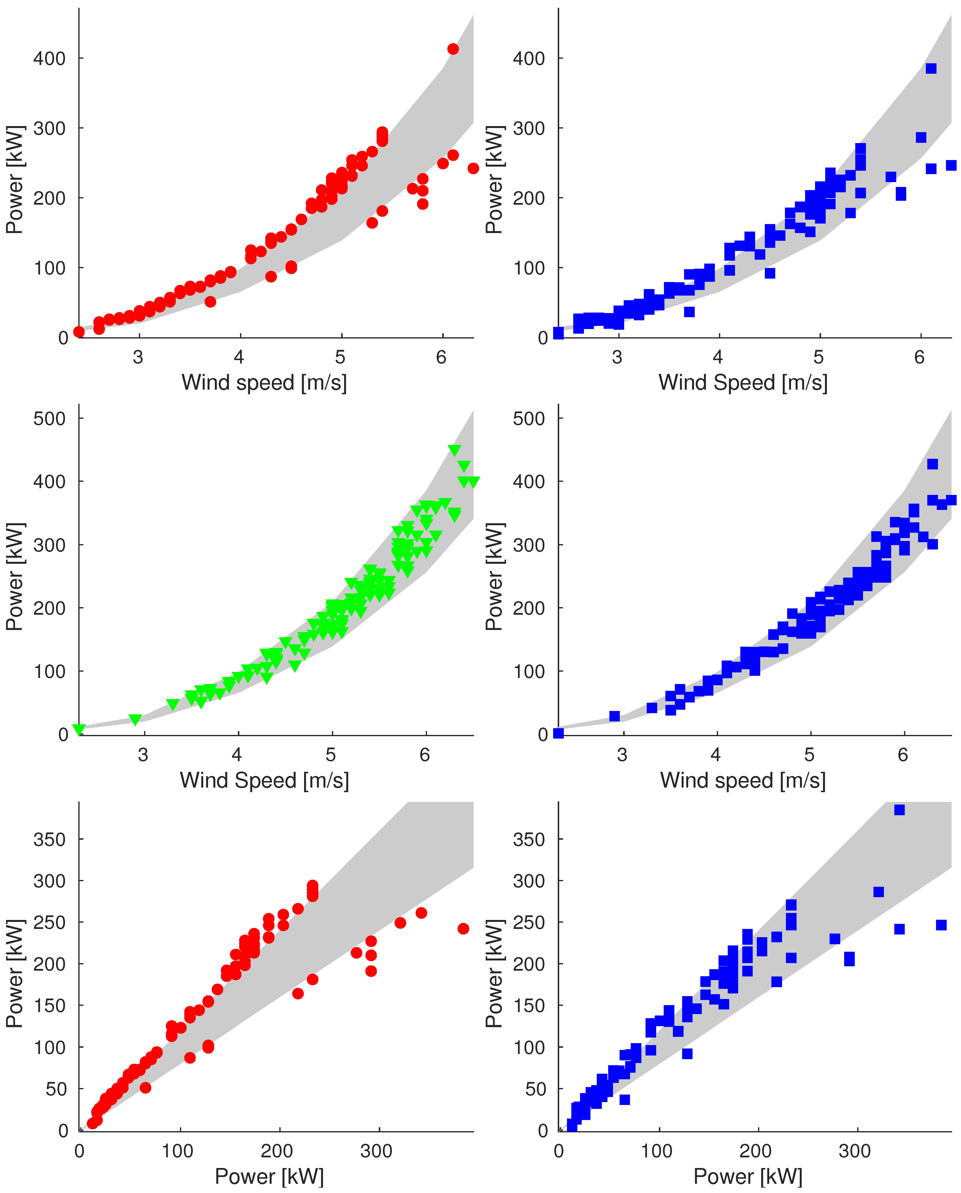
Appendix A.1. Sample_75


Appendix A.2. Sample_90

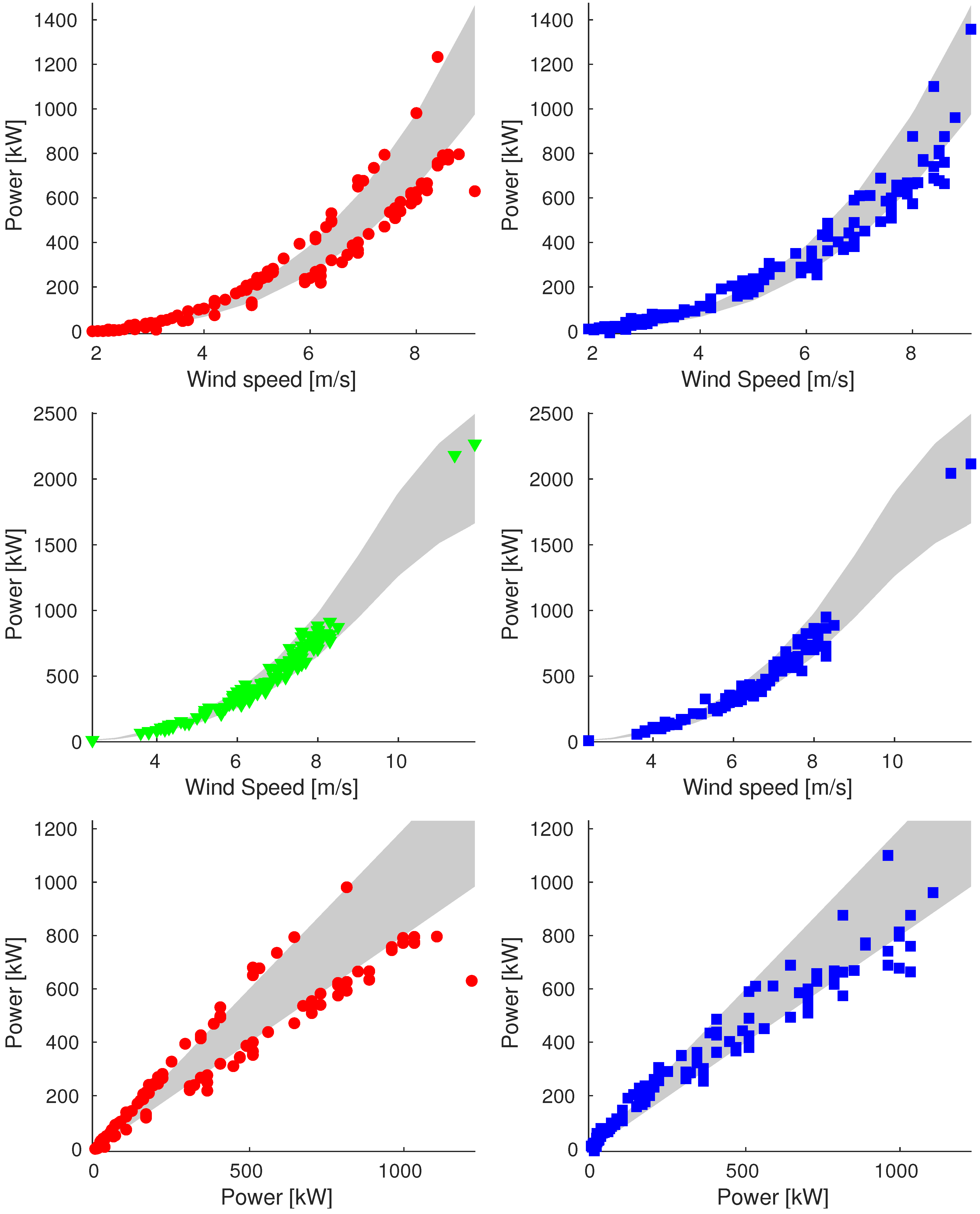
Appendix A.3. Sample_100
References
- Global Wind Report 2022. Global Wind Energy Council. 2022. Available online: https://gwec.net/global-wind-report-2022/ (accessed on 25 November 2022).
- World Energy Transitions Outlook: 1.5 °C Pathway. IRENA. 2022. Available online: https://www.irena.org/publications/2022/mar/world-energy-transitions-outlook-2022 (accessed on 25 November 2022).
- Meyers, J.; Bottasso, C.; Dykes, K.; Fleming, P.; Gebraad, P.; Giebel, G.; Göçmen, T.; van Wingerden, J.W. Wind farm flow control: Prospects and challenges. Wind. Energy Sci. Discuss. 2022, 7, 2271–2306. [Google Scholar] [CrossRef]
- Hu, Y.; Qiao, Y.; Liu, J.; Zhu, H. Adaptive Confidence Boundary Modeling of Wind Turbine Power Curve Using SCADA Data and Its Application. IEEE Trans. Sustain. Energy 2019, 10, 1330–1341. [Google Scholar] [CrossRef]
- Pacheco, J.; Pimenta, F.; Pereira, S.; Cunha, Á.; Magalhães, F. Fatigue Assessment of Wind Turbine Towers: Review of Processing Strategies with Illustrative Case Study. Energies 2022, 15, 4782. [Google Scholar] [CrossRef]
- Superchi, F.; Mati, A.; Pasqui, M.; Carcasci, C.; Bianchini, A. Techno-economic study on green hydrogen production and use in hard-to-abate industrial sectors. IOP J. Phys. Conf. Ser. 2022, 2385, 012054. [Google Scholar] [CrossRef]
- Li, Q.; Cheng, L.; Gao, W.; Gao, D.W. Fully Distributed State Estimation for Power System with Information Propagation Algorithm. J. Mod. Power Syst. Clean Energy 2020, 8, 627–635. [Google Scholar] [CrossRef]
- Tawn, R.; Browell, J.; Dinwoodie, I. Missing data in wind farm time series: Properties and effect on forecasts. Electr. Power Syst. Res. 2020, 189, 106640. [Google Scholar] [CrossRef]
- Mao, Y.; Jian, M. Data completing of missing wind power data based on adaptive BP neural network. In Proceedings of the 2016 International Conference on Probabilistic Methods Applied to Power Systems (PMAPS), Beijing, China, 16–20 October 2016; pp. 1–6. [Google Scholar]
- Salmon, J.; Taylor, P. Errors and uncertainties associated with missing wind data and short records. Wind Energy 2014, 17, 1111–1118. [Google Scholar] [CrossRef]
- Aidan, C.; Afzal, S.; Klaus-Ole, V. The effect of missing data on wind resource estimation. Energy 2011, 36, 4505–4517. [Google Scholar]
- Pinson, P. Wind Energy: Forecasting Challenges for Its Operational Management. Stat. Sci. 2013, 28, 564–585. [Google Scholar] [CrossRef]
- Wang, J.; Song, Y.; Liu, F.; Hou, R. Analysis and application of forecasting models in wind power integration: A review of multi-step-ahead wind speed forecasting models. Renew. Sustain. Energy Rev. 2016, 60, 960–981. [Google Scholar] [CrossRef]
- Liao, W.; Bak-Jensen, B.; Pillai, J.R.; Yang, D.; Wang, Y. Data-Driven Missing Data Imputation for Wind Farms Using Context Encoder. J. Mod. Power Syst. Clean Energy 2021, 10, 964–976. [Google Scholar] [CrossRef]
- Wang, Q.; Luo, K.; Wu, C.; Mu, Y.; Tan, J.; Fan, J. Diurnal impact of atmospheric stability on inter-farm wake and power generation efficiency at neighboring onshore wind farms in complex terrain. Energy Convers. Manag. 2022, 267, 115897. [Google Scholar] [CrossRef]
- Wang, Q.; Luo, K.; Yuan, R.; Wang, S.; Fan, J.; Cen, K. A multiscale numerical framework coupled with control strategies for simulating a wind farm in complex terrain. Energy 2020, 203, 117913. [Google Scholar] [CrossRef]
- Khayati, M.; Lerner, A.; Tymchenko, Z.; Cudré-Mauroux, P. Mind the gap: An experimental evaluation of imputation of missing values techniques in time series. In Proceedings of the VLDB Endowment, Tokyo, Japan, 30 August–4 September 2020; Volume 13, pp. 768–782. [Google Scholar]
- Jones, A.; Keatley, A.; Goulermas, J.; Scott, T.; Turner, P.; Awbery, R.; Stapleton, M. Machine learning techniques to repurpose Uranium Ore Concentrate (UOC) industrial records and their application to nuclear forensic investigation. Appl. Geochem. 2018, 91, 221–227. [Google Scholar] [CrossRef]
- Jia, X.; Dong, X.; Chen, M.; Yu, X. Missing data imputation for traffic congestion data based on joint matrix factorization. Knowl.-Based Syst. 2021, 225, 107114. [Google Scholar] [CrossRef]
- Song, S.; Sun, Y.; Zhang, A.; Chen, L.; Wang, J. Enriching Data Imputation under Similarity Rule Constraints. IEEE Trans. Knowl. Data Eng. 2020, 32, 275–287. [Google Scholar] [CrossRef]
- Breve, B.; Caruccio, L.; Deufemia, V.; Polese, G. RENUVER: A Missing Value Imputation Algorithm based on Relaxed Functional Dependencies. In Proceedings of the EDBT, Edinburgh, UK, 29 March–1 April 2022; pp. 1–52. [Google Scholar]
- Rekatsinas, T.; Chu, X.; Ilyas, I.F.; Ré, C. HoloClean: Holistic Data Repairs with Probabilistic Inference. arXiv 2017, arXiv:1702.00820. [Google Scholar] [CrossRef]
- Lotfi, B.; Mourad, M.; Najiba, M.B.; Mohamed, E. Treatment methodology of erroneous and missing data in wind farm dataset. In Proceedings of the Eighth International Multi-Conference on Systems, Signals & Devices, Sousse, Tunisia, 22–25 March 2011; pp. 1–6. [Google Scholar]
- Agarwal, A.; Amjad, M.J.; Shah, D.; Shen, D. Model agnostic time series analysis via matrix estimation. arXiv 2018, arXiv:1802.09064. [Google Scholar] [CrossRef]
- Ramlatchan, A.; Yang, M.; Liu, Q.; Li, M.; Wang, J.; Li, Y. A survey of matrix completion methods for recommendation systems. Big Data Min. Anal. 2018, 1, 308–323. [Google Scholar]
- Troyanskaya, O.; Cantor, M.; Sherlock, G.; Brown, P.; Hastie, T.; Tibshirani, R.; Botstein, D.; Altman, R.B. Missing value estimation methods for DNA microarrays. Bioinformatics 2001, 17, 520–525. [Google Scholar] [CrossRef]
- Nguyen, L.T.; Kim, J.; Shim, B. Low-rank matrix completion: A contemporary survey. IEEE Access 2019, 7, 94215–94237. [Google Scholar] [CrossRef]
- Fazel, M. Matrix Rank Minimization with Applications. Ph.D. Thesis, Stanford University, Stanford, CA, USA, 2002. [Google Scholar]
- Candès, E.J.; Recht, B. Exact matrix completion via convex optimization. Found. Comput. Math. 2009, 9, 717–772. [Google Scholar] [CrossRef]
- Chatterjee, S. Matrix estimation by universal singular value thresholding. Ann. Stat. 2015, 43, 177–214. [Google Scholar] [CrossRef]
- Cai, J.F.; Candès, E.J.; Shen, Z. A singular value thresholding algorithm for matrix completion. SIAM J. Optim. 2010, 20, 1956–1982. [Google Scholar] [CrossRef]
- Mazumder, R.; Hastie, T.; Tibshirani, R. Spectral regularization algorithms for learning large incomplete matrices. J. Mach. Learn. Res. 2010, 11, 2287–2322. [Google Scholar]
- Bellavia, S.; Gondzio, J.; Porcelli, M. A Relaxed Interior Point Method for Low-Rank Semidefinite Programming Problems with Applications to Matrix Completion. J. Sci. Comput. 2021, 89, 46. [Google Scholar] [CrossRef]
- Bellavia, S.; Gondzio, J.; Porcelli, M. An inexact dual logarithmic barrier method for solving sparse semidefinite programs. Math. Program. 2019, 178, 109–143. [Google Scholar] [CrossRef]
- Recht, B.; Fazel, M.; Parrilo, P.A. Guaranteed minimum-rank solutions of linear matrix equations via nuclear norm minimization. SIAM Rev. 2010, 52, 471–501. [Google Scholar] [CrossRef]
- Toh, K.C.; Yun, S. An accelerated proximal gradient algorithm for nuclear norm regularized linear least squares problems. Pac. J. Optim. 2010, 6, 15. [Google Scholar]
- Ma, S.; Goldfarb, D.; Chen, L. Fixed point and Bregman iterative methods for matrix rank minimization. Math. Program. 2011, 128, 321–353. [Google Scholar] [CrossRef]
- Keshavan, R.H.; Montanari, A.; Oh, S. Matrix completion from a few entries. IEEE Trans. Inf. Theory 2010, 56, 2980–2998. [Google Scholar] [CrossRef]


| Reconst. Rate | RMSE | |||||||||
|---|---|---|---|---|---|---|---|---|---|---|
| Day | RT | CPU | ||||||||
| 26 February | 233 | 536 | 95 | 9.97% | 37.0% | 1.5 | ||||
| 7 May | 247 | 524 | 93 | 6.90% | 24.1% | 1.5 | ||||
| 26 July | 258 | 515 | 91 | 6.54% | 21.9% | 1.5 | ||||
| 19 August | 264 | 510 | 90 | 7.82% | 25.6% | 1.4 | ||||
| 2 September | 317 | 465 | 82 | 10.71% | 29.2% | 1.5 | ||||
| Reconst. Rate | RMSE | |||||||||
|---|---|---|---|---|---|---|---|---|---|---|
| Day | RT | CPU | ||||||||
| 16 May | 115 | 637 | 112 | 7.59% | 57.1% | 1.4 | ||||
| 18 June | 165 | 594 | 105 | 7.91% | 41.4% | 1.6 | ||||
| 18 August | 199 | 565 | 100 | 6.34% | 27.5% | 1.5 | ||||
| 26 August | 114 | 638 | 112 | 5.93% | 45.0% | 1.6 | ||||
| 24 September | 119 | 633 | 112 | 8.21% | 59.6% | 1.6 | ||||
| Reconst. Rate | RMSE | |||||||||
|---|---|---|---|---|---|---|---|---|---|---|
| Day | RT | CPU | ||||||||
| 10 April | 43 | 698 | 123 | 1.34% | 26.9% | 1.5 | ||||
| 2 June | 12 | 724 | 128 | 0.93% | 67.0% | 1.7 | ||||
| 15 September | 81 | 666 | 117 | 5.97% | 63.7% | 1.5 | ||||
| 16 October | 11 | 725 | 128 | 0.89% | 69.6% | 1.7 | ||||
| 11 December | 29 | 710 | 125 | 1.70% | 50.6% | 1.6 | ||||
Disclaimer/Publisher’s Note: The statements, opinions and data contained in all publications are solely those of the individual author(s) and contributor(s) and not of MDPI and/or the editor(s). MDPI and/or the editor(s) disclaim responsibility for any injury to people or property resulting from any ideas, methods, instructions or products referred to in the content. |
© 2023 by the authors. Licensee MDPI, Basel, Switzerland. This article is an open access article distributed under the terms and conditions of the Creative Commons Attribution (CC BY) license (https://creativecommons.org/licenses/by/4.0/).
Share and Cite
Silei, M.; Bellavia, S.; Superchi, F.; Bianchini, A. Recovering Corrupted Data in Wind Farm Measurements: A Matrix Completion Approach. Energies 2023, 16, 1674. https://doi.org/10.3390/en16041674
Silei M, Bellavia S, Superchi F, Bianchini A. Recovering Corrupted Data in Wind Farm Measurements: A Matrix Completion Approach. Energies. 2023; 16(4):1674. https://doi.org/10.3390/en16041674
Chicago/Turabian StyleSilei, Mattia, Stefania Bellavia, Francesco Superchi, and Alessandro Bianchini. 2023. "Recovering Corrupted Data in Wind Farm Measurements: A Matrix Completion Approach" Energies 16, no. 4: 1674. https://doi.org/10.3390/en16041674
APA StyleSilei, M., Bellavia, S., Superchi, F., & Bianchini, A. (2023). Recovering Corrupted Data in Wind Farm Measurements: A Matrix Completion Approach. Energies, 16(4), 1674. https://doi.org/10.3390/en16041674