Investigating Empirical Mode Decomposition in the Parameter Estimation of a Three-Section Winding Model ^†

Abstract

Parameter estimation represents an important aspect of modeling electromagnetic systems, and a wide range of parameter estimation strategies has been explored in literature. Most parameter estimation methodologies make use of either time-domain or frequency-domain responses as measured from the terminals of the device under test. Very limited research has, however, been conducted into exploring the use of modal decomposition strategies on the time-domain waveforms for parameter estimation applications. In this paper, the use of Empirical Mode Decomposition for estimating the parameters of a three-section lumped parameter transformer model is explored. A novel approach is proposed to define the optimization cost function in terms of the intrinsic modes of simulated time-domain waveforms. The results are compared with results obtained using classical time-domain and frequency-domain approaches. It is shown through an impulse response test that weighting the modes obtained from the Inferred Empirical Mode Decomposition approach presented in this work offers advantages in terms of accurately representing the target model transfer function dynamics and can assist in interpreting the various dynamic modes associated with the target model.

1. Introduction

The harmonics introduced by inverter-based renewable generation mean that transformers are being operated at voltages with a high level of high-frequency harmonic content [1]. This creates a need for accurate wideband equivalent-circuit transformer models that represent the expected transfer function characteristics under these operating conditions, especially for simulation studies aimed at characterizing system behavior. Additionally, being able to model transformer responses during transient conditions allows for early detection of failure and electrical faults using techniques such as Frequency Response Analysis (FRA) [2]. Aguglia [3] highlights that a model with good parameter accuracy is important to a transformer designer, while for control purposes, an accurate mathematical model relating the input to the output of a system is sufficient.

High frequency modeling of transformer windings ideally requires distributed winding models. These models are, however, commonly approximated using lumped-parameter equivalent circuit models, and the topologies of these lumped parameter models have been studied extensively in literature [4,5]. Various methodologies have been proposed for estimating the parameters of wideband transformer models. Keyhani [4,6] performed maximum likelihood estimation on a six-section transformer winding model and concluded that unique solutions can only be estimated if the initial values are close to the target values, or if sectional voltage measurements were included. Brozio [5] used a constrained Sequential Quadratic Programming (SQP) optimization algorithm to estimate the parameters of a two-winding power transformer from measured frequency responses. Time-domain signals were not employed due to computational limitations, and the overall simplicity of representing the frequency responses analytically. In a more recent contribution, Chanane [7,8,9] applied metaheuristic optimization algorithms, such as Particle Swarm Optimization (PSO) [10], Crow Search Optimization (CSO) [11], and Grey Wolf Algorithm (GWA) [12], to estimate the parameters of a fully interleaved continuous-disc winding. The parameter estimation process was simplified by making use of measured values for the DC resistance, equivalent inductance, and effective capacitance of the transformer winding.

Empirical Mode Decomposition (EMD), proposed by Huang, represents a methodology for decomposing a multi-modal signal into simpler components known as Intrinsic Mode Functions (IMFs), which can be used to extract features from nonlinear and non-stationary waveforms [13,14]. Alternative noise-assisted EMD methods, such as Ensemble Empirical Mode Decomposition (EEMD) and signal masking techniques, have been subsequently proposed to address the issue of mode-mixing [13,14,15]. EMD and variations thereof have been used extensively in literature for transformer vibration analysis [16,17,18,19]. No existing research applies EMD in the parameter estimation of transformer winding or complete transformer models.

This paper investigates the use of EMD for estimating the parameters of a three-section lumped-parameter transformer winding model. The main research objective of the work is to explore how the classical parameter estimation methodologies can be amended to incorporate EMD, and whether EMD can improve the performance of these approaches. As a second objective, the work investigates the performance of the Pseudo-Random Impulse Sequence (PRIS) [20,21,22] for the parameter estimation of transformer models.

The model is perturbed using a PRIS, and the simulated time-domain voltage waveforms of the winding are decomposed into IMFs. A novel approach is proposed to derive the cost function from these IMFs, the approach is further expanded to investigate weighting of the derived intrinsic modes. The accuracy of the estimated model parameters is interpreted by comparing the impulse responses of the targeted and estimated models in addition to consideration of classical error metrics.

This paper is structured as follows. In Section 2, the transformer winding model used for the study is presented together with its analytical input impedance frequency response. Section 3 presents the PRIS source used to perturb the transformer winding. Section 4 discusses the parameter estimation methodologies being applied. The different cost function formulations used for the parameter estimation algorithm are presented in Section 5. Section 6 presents the results obtained from the different parameter estimation approaches. Additional analysis and results are also presented to provide insight into the results. The paper is concluded in Section 7 with recommendations for further research.

2. Transformer Winding Model

The investigation targets the model proposed by Chanane [8] for a fully interleaved continuous-disc winding with 5 discs, consisting of 30 turns per disc, of copper conductor with a cross-sectional area of 10 mm². The winding features an insulated core with insulation thickness and duct spacing corresponding to a 30 kV insulation rating. Figure 1 shows the model topology, while

Table 1. Parameter values for the model shown in Figure 1.

${\mathit{R}}_{\mathit{s}}$	${\mathit{C}}_{\mathit{s}}$	${\mathit{C}}_{\mathit{g}}$	${\mathit{L}}_{\mathit{s}}$	${\mathit{K}}_{12}$	${\mathit{K}}_{13}$	${\mathit{K}}_{23}$
$83m\mathsf{\Omega }$	$970p\mathrm{F}$	$1.6n\mathrm{F}$	$181\mu \mathrm{H}$	$0.8792$	$0.8729$	$0.8564$

summarizes the target model parameters used by Chanane and in this investigation [8]. The model has a total of 16 parameters to be estimated. These can, however, be reduced by assuming that the winding sections have the same physical dimensions such that $R_1$ = $R_2$ = $R_3$ = $R_s$ and $L_1$ = $L_2$ = $L_3$ = $L_s$. The dimensions between sections are also assumed to be similar, and thus $C_{12}$ = $C_{23}$ = $C_{34}$ = $C_s$. It is furthermore assumed that the capacitances from the individual sections to ground are equal, aside from the sections closest to the grounded core and tank, which is assumed to be half the ground capacitance, so $C_{g1}$ = $C_{g4}$ = $\frac{C_g}{2}$ and $C_{g2}$ = $C_{g3}$ = $C_g$. These assumptions are used extensively in literature and have shown to accurately model the wideband responses of the transformer winding [7,8,9,23,24,25].

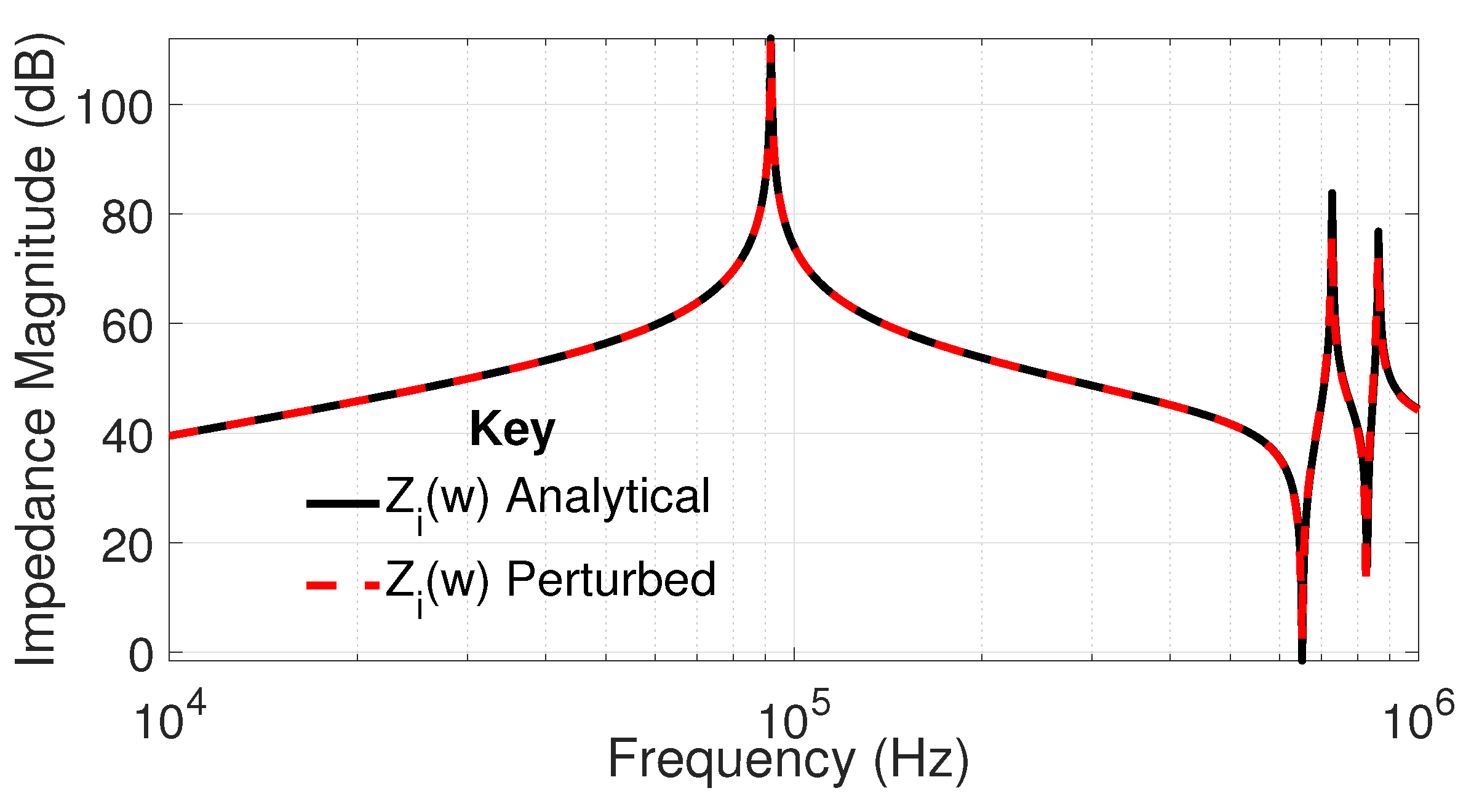
Analytical Input Impedance Frequency Response

The input impedance $Z_i\left(s\right)$ of the circuit model shown in Figure 1 can be derived from the impedance matrix $\mathbf{Z}$ of the model, using the relationship

$$Z_i\left(s\right)=\frac{V_{in}\left(s\right)}{I_{in}\left(s\right)}=\frac{{\Delta }_{\mathbf{Z}}}{C_{\mathbf{Z}(7,7)}},$$

(1)

where ${\Delta }_{\mathbf{Z}}$ denotes the determinant of $\mathbf{Z}$ and $C_{\mathbf{Z}(7,7)}$ denotes the (7,7)-th cofactor of $\mathbf{Z}$. The resulting analytical expression for the transfer function $Z_i\left(s\right)$ can be expressed in the form

$$\begin{array}{c}\hfill Z_i\left(s\right)=\frac{{\alpha }_1{s}^5+{\alpha }_2{s}^4+{\alpha }_3{s}^3+{\alpha }_4{s}^2+{\alpha }_{5}s+{\alpha }_6}{{\beta }_1{s}^6+{\beta }_2{s}^5+{\beta }_3{s}^4+{\beta }_4{s}^3+{\beta }_5{s}^2+{\beta }_{6}s+{\beta }_7},\end{array}$$

(2)

where $\alpha$ and $\beta$ denote constant coefficients defined in terms of the circuit parameters.

3. Target Model Perturbation

The winding model is excited at the terminals in MATLAB Simulink using the PRIS perturbation arrangement presented in Figure 2. The operation of the PRIS source is extensively discussed in literature [20,21,22], it is shown that the spectral content and SNR of the PRIS source is controllable. The controllability makes it well suited for exciting electromagnetic equipment such as transformer systems where direct current or low-frequency components of the perturbation signal are undesirable as these can lead to core saturation [20,21,22]. The RLC values of the source, i.e., $R_{pris}=150\Omega$, $L_{pris}=4$ mH and $C_{pris}=1\mathsf{\mu }\mathrm{F}$ are obtained by following the source design considerations presented in [20], and $V_{DC}=100$ V.

The PRIS is generated using a Pseudo-Random Binary Sequence (PRBS) clock frequency, $f_{clk}$, of 100 kHz, and a 12th order topology for frequency response measurements and a 6th order topology for time-domain measurements. The higher order PRBS for the frequency-domain measurements is required to accommodate a high frequency resolution over a wide frequency band. Figure 3 shows typical simulated time-domain waveforms of the input voltage and input current, together with the PRBS gating signals. The simulation is run for three 6th order topology cycles. In order to remove the effects of the initial transients in the simulation, only the last sequence is captured for analysis.

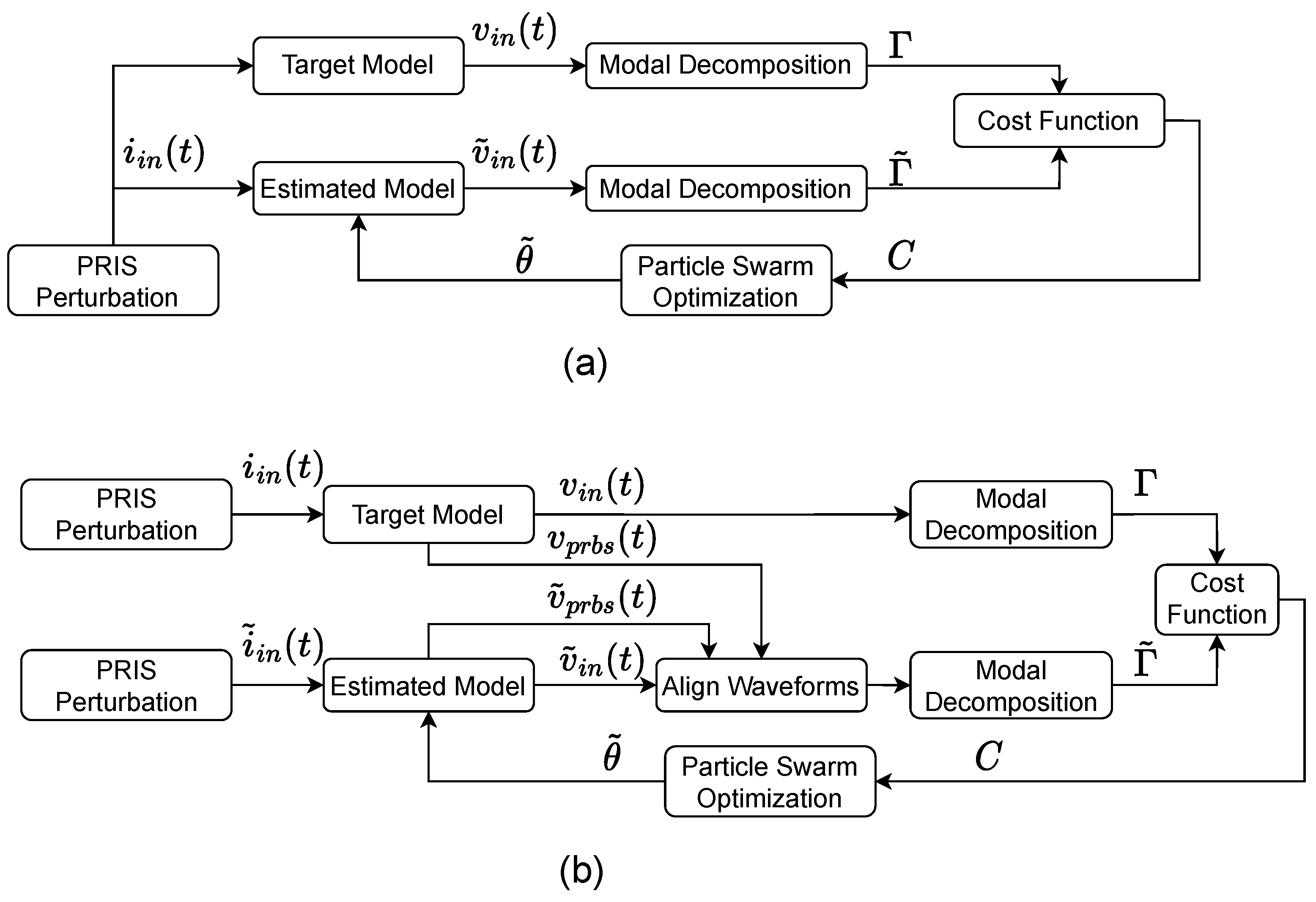
4. Parameter Estimation Methodology

The parameter estimation approaches target the parameter vector given in (3), where the parameters are normalized by applying the normalization constants given in (4). The optimization bounds for parameters other than the coupling coefficients are chosen to be an entire order of magnitude so as to assume little a priori information about the parameter values. The coupling coefficient bounds are selected close to unity to reflect the assumption of a well designed transformer [26].

Table 2. Parameter Boundary Constraints.

Parameters	${\mathit{R}}_{\mathit{s}}$	${\mathit{C}}_{\mathit{s}}$	${\mathit{C}}_{\mathit{g}}$	${\mathit{L}}_{\mathit{s}}$	${\mathit{K}}_{12}$	${\mathit{K}}_{13}$	${\mathit{K}}_{23}$
Lower Bound	1	1	1	1	85	85	85
Upper Bound	1000	1000	1000	1000	95	95	95

summarizes the bounds of the search space adopted in the investigation.

$$\begin{array}{cc}\hfill \theta & =[R_s,C_s,C_g,L_s,k_{12},k_{13},k_{23}]\hfill \end{array}$$

(3)

$$\begin{array}{cc}\hfill {\theta }_{norm}& =[{10}^{-3},{10}^{-12},{10}^{-9},{10}^{-6},{10}^{-2},{10}^{-2},{10}^{-2}]\hfill \end{array}$$

(4)

Figure 4 and Figure 5 present an overview of the parameter estimation strategies implemented in the investigation. In simulation, the target model is perturbed using a PRIS source [20]. In practice, it cannot be guaranteed that the time-domain samples obtained from the device under test align perfectly with the samples obtained through simulation of the estimated model. Two strategies to align these time-domain waveforms are considered. The first strategy, as presented in Figure 4a and Figure 5a, uses the sampled input current, $i_{in}\left(t\right)$, produced during the target model perturbation as an input to the estimated model. The second strategy, as presented in Figure 4b and Figure 5b, simulates the target and estimated model PRIS perturbation arrangements separately, and then aligns the waveforms by aligning the bipolar PRBS voltages produced by the H-Bridge, $v_{prbs}\left(t\right)$, in each simulation.

The initial studies considered various optimisation algorithms, including interior-point, patternsearch, particle swarm and genetic algorithm. The particle swarm optimization algorithm, which is a global solver that generates a population of points to find a global minimum in a widely bounded search space, is used throughout the investigation [8]. The algorithm is chosen based on the assumption that limited a priori knowledge is available on the model parameters to be estimated and the superior runtimes in comparison to the genetic algorithm. The algorithm runs 250 search iterations, with a population of 1000 points generated using a random seed. After the global optimization procedure is completed, the optimization results are refined using a local solver, fmincon. The classical time-domain approach to parameter estimation, whereby the measured output voltage waveforms from the target and estimated models are compared and used in a cost function formulation, is presented in Figure 4.

Figure 5 presents the proposed EMD approach, whereby the time-domain voltage waveforms are first decomposed into IMFs, from which the cost function is derived. Cost functions defined in terms of both Root Mean Squared Error (RMSE) and correlation coefficient ($\rho$) based metrics are implemented for all approaches.

Three implementations of modal decomposition are investigated. The first performs standard EMD on the target model and estimated model voltage waveforms, and formulates the cost function in terms of the resulting IMFs and residuals. The second computes inferred IMFs to represent the estimated model, from which the cost function is derived. The third derives the cost function from weighted inferred IMFs to represent the estimated model.

5. Parameter Estimation Cost Function Formulations

5.1. Frequency-Domain Approach

To validate the Simulink model, the frequency response of the input impedance of the target model is obtained from the simulated input voltage and input current signals during PRIS perturbation using Welch’s method [27], and compared to the analytical frequency response. Figure 6 shows the frequency responses of the input impedance of the target model obtained analytically and through perturbation. The responses exhibit a strong correlation between the analytical and estimated frequency responses.

For the frequency-domain parameter estimation, the RMSE based cost function, $C_{rmse}^z$, is calculated as

$$\begin{array}{c}\hfill C_{rmse}^z=\sqrt{\frac{1}{N_k}\sum _{k=1}^{N_k}{\left(ϵ\left({\omega }_k\right)\right)}^2},\end{array}$$

(5)

where

$$\begin{array}{c}\hfill ϵ\left({\omega }_k\right)={log}_{10}{Z}_i\left({\omega }_k\right)-{log}_{10}\widetilde{Z_i}\left({\omega }_k\right),k=1,...,N_k.\end{array}$$

(6)

The error $ϵ\left({\omega }_k\right)$ between the input impedance frequency responses of the target model $Z_i\left(\omega \right)$ and estimated model $\widetilde{Z_i}\left(\omega \right)$ is calculated on a point-by-point basis for each frequency sample up to $N_k$ samples. The sample frequencies ${\omega }_k$ are distributed logarithmically such that the contributions from $ϵ\left({\omega }_k\right)$ to the cost function are distributed equitably across the frequency range of interest.

The correlation coefficient metric is used to compute the correlation based cost function, $C_{\rho }^z$, as

$$\begin{array}{c}\hfill C_{\rho }^z=-\rho \{Z_i\left(\omega \right),{\tilde{Z}}_i\left(\omega \right)\}+1\end{array}$$

(7)

by adjusting the correlation coefficient, $\rho$, between $Z_i\left(\omega \right)$ and ${\tilde{Z}}_i\left(\omega \right)$ such that a value of zero represents a perfect match in frequency responses.

5.2. Time-Domain Approach

The time-domain target voltage waveform, shown in Figure 3, is defined by $v_{in}\left(t\right)$. The cost function using the RMSE metric, $C_{rmse}^v$, is calculated as

$$\begin{array}{c}\hfill C_{rmse}^v=\sqrt{\frac{1}{N_k}\sum _{k=1}^{N_k}{\left(ϵ\left(t_k\right)\right)}^2},\end{array}$$

(8)

where

$$\begin{array}{c}\hfill ϵ\left(t_k\right)=v_{in}\left(t_k\right)-{\tilde{v}}_{in}\left(t_k\right),k=1,2,...,N_k.\end{array}$$

(9)

The errors between the voltage waveforms of the target model $v_{in}\left(t\right)$, and estimated model ${\tilde{v}}_{in}\left(t\right)$ are calculated on a point-by-point basis for each time sample $t_k$ up to $N_k$ samples.

Similar to the frequency-domain approach in (7), the correlation coefficient based cost function, $C_{\rho }^v$, is defined in terms of the correlation between the target and estimated voltage waveforms as

$$\begin{array}{c}\hfill C_{\rho }^v=-\rho \{v_{in}\left(t\right),{\tilde{v}}_{in}\left(t\right)\}+1.\end{array}$$

(10)

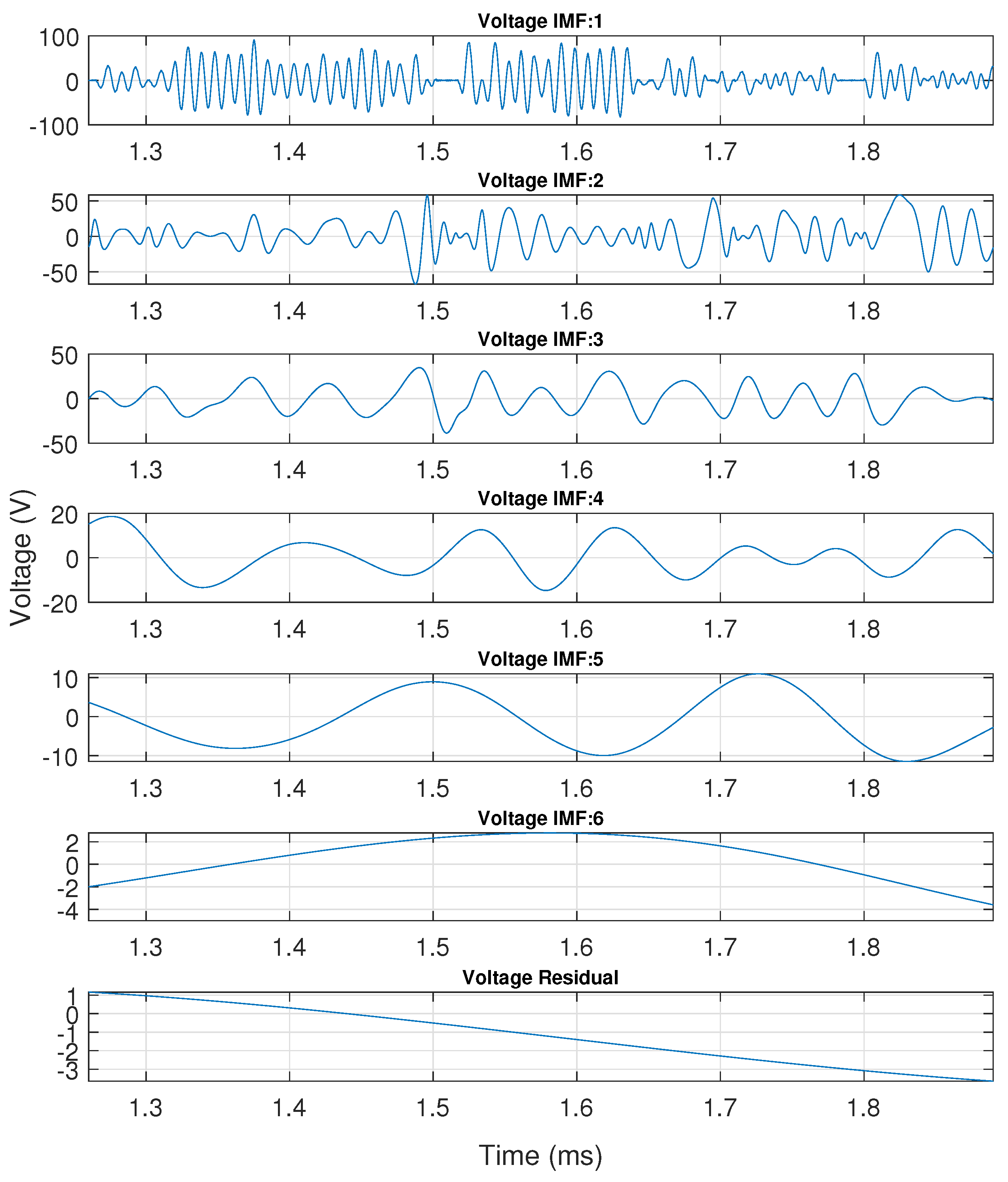
5.3. Empirical Mode Decomposition Approach

The simulated time-domain voltage waveform shown in Figure 3 is decomposed into IMFs using EMD [13]. This yields six IMFs and one residual, as shown in Figure 7.

The voltage waveforms associated with the target model and estimated model, denoted by $v\left(t\right)$ and $\tilde{v}\left(t\right)$, respectively, can be represented by the relationships

$$\begin{array}{cc}\hfill v\left(t\right)=& \sum _{i=1}^{N_i}{v}_i^m\left(t\right)+v^r\left(t\right)\hfill \end{array}$$

(11)

and

$$\begin{array}{cc}\hfill \tilde{v}\left(t\right)=& \sum _{i=1}^{{\tilde{N}}_i}{\tilde{v}}_i^m\left(t\right)+{\tilde{v}}^r\left(t\right),\hfill \end{array}$$

(12)

where $v_i^m\left(t\right)$ and ${\tilde{v}}_i^m\left(t\right)$ denote the $i^{th}$ IMFs, $N_i$ and ${\tilde{N}}_i$ denotes the total number of IMFs, and $v^r\left(t\right)$ and ${\tilde{v}}^r\left(t\right)$ denote the residuals, of the target model and estimated model, respectively. The IMFs and residuals for the target model and estimated model are represented by the sets $\mathsf{\Gamma }$ and $\tilde{\mathsf{\Gamma }}$, respectively. The set sizes of the target model and estimated model are denoted as $N_r$ and ${\tilde{N}}_r$, respectively, as shown in (13) and (14).

$$\begin{array}{c}\hfill \mathsf{\Gamma }=\{{\gamma }_r\left(t\right)r=1,2...N_r\}\end{array}$$

(13)

$$\begin{array}{c}\hfill \tilde{\mathsf{\Gamma }}=\{\widetilde{{\gamma }_r}\left(t\right)r=1,2...{\tilde{N}}_r\}\end{array}$$

(14)

The set with fewer IMFs is padded with zeros such that the sets are of equal length and can be compared.

The Normalized RMSE (NRMSE) based cost function, $C_{nrmse}^m$, for the Empirical Mode Decomposition approach is calculated as

$$\begin{array}{c}\hfill C_{nrmse}^m=\sum _{r=1}^{N_r}\frac{1}{{\psi }_r}\sqrt{\frac{1}{N_k}\sum _{k=1}^{N_k}{\left({ϵ}_r\left(t_k\right)\right)}^2},\end{array}$$

(15)

where

$$\begin{array}{c}\hfill {ϵ}_r\left(t_k\right)={\gamma }_r\left(t_k\right)-{\tilde{\gamma }}_r\left(t_k\right).\end{array}$$

(16)

The error ${ϵ}_r\left(t_k\right)$ is thus defined as the difference between the $r^{th}$ waveforms in sets $\mathsf{\Gamma }$ and $\tilde{\mathsf{\Gamma }}$ at sample time $t_k$.

The respective errors are then normalized by applying the normalization constant

$$\begin{array}{c}\hfill {\psi }_r=\max \left\{{\gamma }_r\left(t\right)\right\}-\min \left\{{\gamma }_r\left(t\right)\right\},\end{array}$$

(17)

where $\max \left\{{\gamma }_r\left(t\right)\right\}$ and $\min \left\{{\gamma }_r\left(t\right)\right\}$ denote the maximum and minimum amplitudes of the $r^{th}$ target IMF waveform, respectively. This normalization is required to counter biasing of the cost function towards waveforms with higher amplitude, as the measurement set consists of waveforms with varying amplitudes. The normalization constant is omitted in cases when the target data set is zero-padded as it results in a ${\psi }_r=0$.

In the case of the correlation coefficient based cost function, the larger set between the target and estimated sets is truncated to the length of the shorter set, denoted by $N_s$, as correlation coefficient metrics do not allow for zero-padded waveforms. Due to this manipulation, a variance occurs in the number of IMFs from iteration to iteration in the optimization procedure, and the result is thus normalized by $N_s$. The correlation coefficient based cost function, $C_{\rho }^m$, is thus defined as

$$\begin{array}{c}\hfill C_{\rho }^m=\frac{1}{N_s}\sum _{r=1}^{N_s}[-\rho \{{\gamma }_r\left(t\right),{\tilde{\gamma }}_r\left(t\right)\}+1].\end{array}$$

(18)

5.4. Inferred Empirical Mode Decomposition

In this method, the IMFs produced by the estimated waveforms are never computed. Instead, a set of inferred IMFs (iIMFs) is produced to represent the estimated model. The target model set, $\mathsf{\Gamma }$, remains the same as in (13). The $r^{th}$ iIMF, ${\tilde{v}}_r^i\left(t\right)$, for the estimated model voltage waveform, $\tilde{v}\left(t\right)$, and is determined by subtracting waveforms 1 to $r-1$ and waveforms $r+1$ to $N_r$ in $\mathsf{\Gamma }$ from $\tilde{v}\left(t\right)$. This is represented by the relationship

$$\begin{array}{cc}\hfill {\tilde{v}}_r^i\left(t\right)=& \tilde{v}\left(t\right)-\sum _{k=1}^{r-1}{\gamma }_k\left(t\right)-\sum _{k=r+1}^{N_r}{\gamma }_k\left(t\right).\hfill \end{array}$$

(19)

The estimated model set, while in the same form as in (14), consists of the iIMFs of the estimated voltage waveform as given in (19). The number of iIMFs produced is always the same as the number of target IMFs, and the length of $\tilde{\mathsf{\Gamma }}$ thus becomes $N_r$, such that

$$\begin{array}{c}\hfill \tilde{\mathsf{\Gamma }}=\{\widetilde{{\gamma }_r}\left(t\right)r=1,2...N_r\}.\end{array}$$

(20)

This decomposition approach creates a set of iIMFs that each contain the error dynamics of the estimated signal, whilst also containing the corresponding target IMF dynamics that are present in the estimated waveform. The cost function for the NRMSE based metric is calculated as

$$\begin{array}{c}\hfill C_{nrmse}^i=\sum _{r=1}^{N_r}\frac{1}{{\psi }_r}\sqrt{\frac{1}{N_k}\sum _{k=1}^{N_k}{\left({ϵ}_r\left(t_k\right)\right)}^2},\end{array}$$

(21)

where the errors, ${ϵ}_r\left(t_k\right)$, and normalization constants, ${\psi }_r$, are defined as in (16) and (17), respectively.

The correlation coefficient based cost function in the context of the Inferred EMD (IEMD) approach does not require truncation of the IMFs nor normalization. The cost function $C_{\rho }^i$ is thus reduced to the form

$$\begin{array}{c}\hfill C_{\rho }^i=\sum _{r=1}^{N_r}[-\rho \{{\gamma }_r\left(t\right),{\tilde{\gamma }}_r\left(t\right)\}+1].\end{array}$$

(22)

5.5. Weighted Inferred Empirical Mode Decomposition

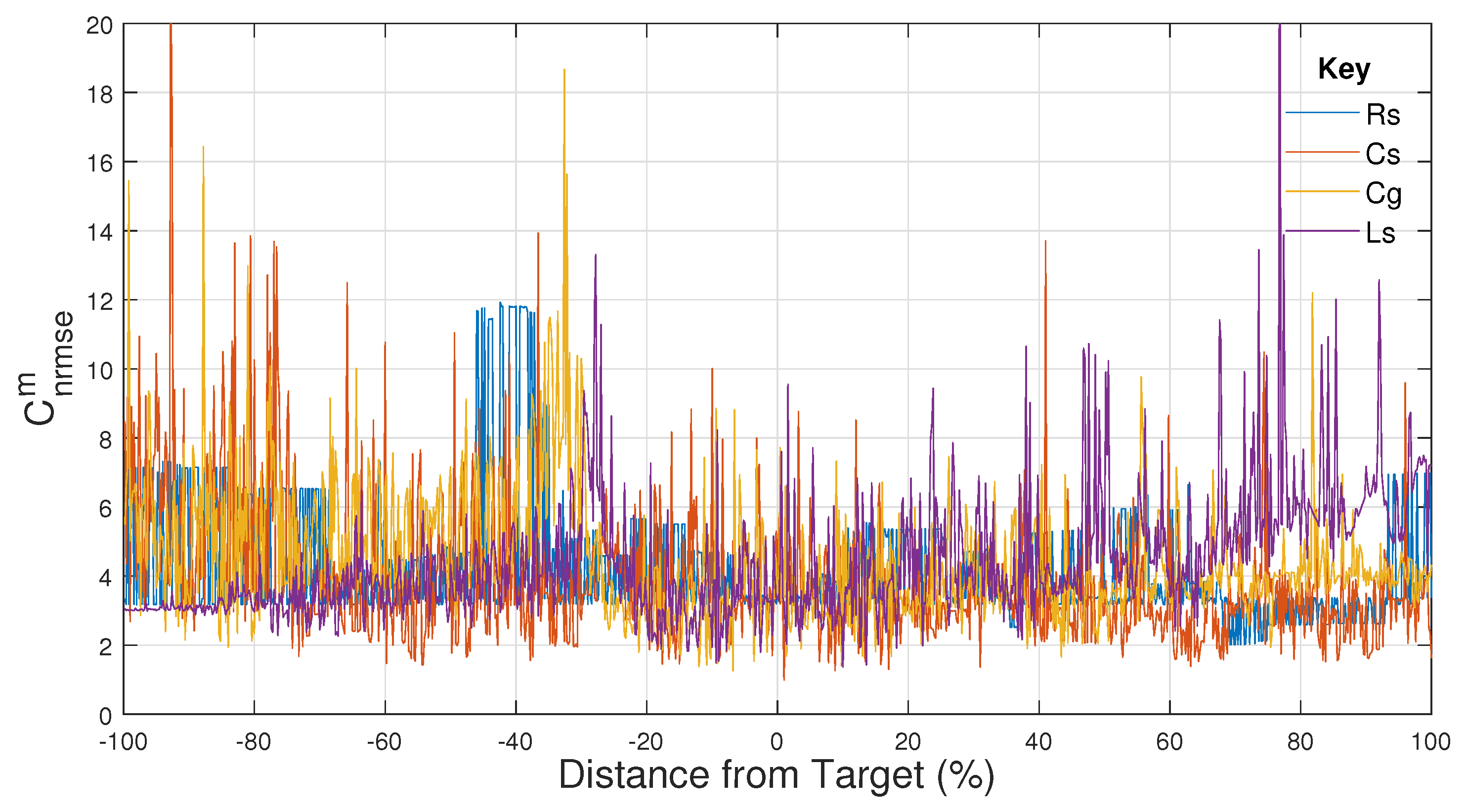
In this approach, the set of correlation coefficients between the target model IMF waveform and the respective iIMF waveform of the estimated model are weighted using a binary weighting vector, $v\left(r\right)$. The weighted correlation coefficient cost function is defined as

$$\begin{array}{c}\hfill C_{\rho }^{wi}=\sum _{r=1}^{N_r}v\left(r\right)[-\rho \{{\gamma }_r\left(t\right),{\tilde{\gamma }}_r\left(t\right)\}+1],\end{array}$$

(23)

where $v\left(r\right)$ is set to either 0 or 1 for the $r^{th}$ waveform in both the target model and estimated model sets. This allows various combinations of correlation coefficients between the IMFs and iIMFs to be included in the cost function formulation. The residual IMF waveform in the set of target model IMFs predominantly contains low-order dynamics. It is expected that the model parameters to not have a significant effect on the low-frequency dynamics, as the resonant points are located above 10 kHz. The residual IMF is therefore excluded in the weighted cost function formulation.

6. Results

Table 3. Estimated Parameter Error Percentages obtained through the Frequency-Domain Approach.

Approach	Frequency-Domain
Cost Function	${\mathit{C}}_{\mathbf{rmse}}^{\mathit{z}}$	${\mathit{C}}_{\mathit{\rho }}^{\mathit{z}}$
$R_s(\mathrm{err}\%)$	−242.50	45.23
$C_s(\mathrm{err}\%)$	−3.09	−0.50
$C_g(\mathrm{err}\%)$	0.67	37.50
$L_s(\mathrm{err}\%)$	2.55	−40.25
$K_{12}(\mathrm{err}\%)$	−8.83	−3.73
$K_{13}(\mathrm{err}\%)$	0.03	-8.80
$K_{23}(\mathrm{err}\%)$	−5.29	−6.70
Runtime (h)	29.88	11.81

presents the results of the frequency-domain parameter estimation investigations, while

Table 4. Estimated Model Parameter Error Percentages obtained through the Time Domain Approaches.

Approach	Time-Domain				Empirical Mode Decomposition				Inferred Empirical Model Decomposition
Alignment	Strategy 1		Strategy 2		Strategy 1		Strategy 2		Strategy 1		Strategy 2
Cost Function	${\mathit{C}}_{\mathbf{rmse}}^{\mathit{v}}$	${\mathit{C}}_{\mathit{\rho }}^{\mathit{v}}$	${\mathit{C}}_{\mathbf{rmse}}^{\mathit{v}}$	${\mathit{C}}_{\mathit{\rho }}^{\mathit{v}}$	${\mathit{C}}_{\mathbf{nrmse}}^{\mathit{m}}$	${\mathit{C}}_{\mathit{\rho }}^{\mathit{m}}$	${\mathit{C}}_{\mathbf{nrmse}}^{\mathit{m}}$	${\mathit{C}}_{\mathit{\rho }}^{\mathit{m}}$	${\mathit{C}}_{\mathbf{nrmse}}^{\mathit{i}}$	${\mathit{C}}_{\mathit{\rho }}^{\mathit{i}}$	${\mathit{C}}_{\mathbf{nrmse}}^{\mathit{i}}$	${\mathit{C}}_{\mathit{\rho }}^{\mathit{i}}$
$R_s(\mathrm{err}\%)$	1.14	83.13	−392.75	4.62	36.90	−941.37	−575.99	−395.22	1.14	−84.61	−392.63	−101.221
$C_s(\mathrm{err}\%)$	−1.91	47.17	−2.01	−0.93	−3.03	25.25	−2.30	−3.03	−1.91	21.58	0.99	10.62
$C_g(\mathrm{err}\%)$	−0.59	−723.11	1.30	8.31	−59.55	37.50	−33.19	34.50	−0.59	−3.74	−0.17	−1.45
$L_s(\mathrm{err}\%)$	1.73	86.26	1.90	−8.80	33.47	−51.22	26.99	−74.00	1.73	−0.91	1.77	1.47
$K_{12}(\mathrm{err}\%)$	−4.78	−4.85	−3.60	2.31	−5.03	0.42	−5.03	−5.66	−4.78	0.67	−1.15	−2.24
$K_{13}(\mathrm{err}\%)$	−3.15	−5.45	2.63	1.15	2.50	−3.10	−7.94	0.33	−3.15	1.88	−3.64	2.43
$K_{23}(\mathrm{err}\%)$	0.53	−8.03	−8.63	−4.93	−0.50	−0.41	−6.46	0.65	0.53	0.74	−3.66	−6.36
Runtime (h)	12.32	4.31	6.66	6.22	5.92	1.76	14.65	9.07	8.33	8.87	6.72	9.49

presents the results of the parameter estimation investigations that utilise the time-domain, EMD and IEMD waveforms. The results are presented as parameter error percentages, where the error (err%) of the respective parameters is calculated using the relationship

$$\begin{array}{c}\hfill \mathrm{err}\%\left(n\right)=\frac{\theta \left(n\right)-\tilde{\theta }\left(n\right)}{\theta \left(n\right)}\times 100[\%],\end{array}$$

(24)

where $\tilde{\theta }$ denotes the final estimated parameter value and $\theta$ denotes the target value of the parameter, as presented in Table 1.

The frequency-domain RMSE based optimization yields errors below 10% for all parameters aside from $R_s$. Parameter $R_s$ does not influence the cost function significantly, as it predominantly affects the damping at the resonant points of the frequency response. In considering Table 3 and Table 4, it is observed that the run times of frequency-domain parameter estimation, in most cases, are longer compared to time-domain and modal decomposition based approaches. This is attributed to the need for longer simulation times to obtain a high frequency resolution over a wide frequency band.

It is clear from Table 4 that cost functions using the EMD approach are not able to obtain parameters as accurately as the classical time-domain approach. This is attributed to the content within each IMF being dependent on the dynamics present in the original signal. EMD does not guarantee the presence of specific modes within a specific IMF. Although the presence of certain modes within the estimated waveform may be correct, it cannot be predicted which IMF these will be decomposed into. This characteristic makes the optimization challenging when only comparing the $n^{th}$ IMF of the target with the $n^{th}$ IMF of the estimated waveforms. The EMD approach is thus very sensitive to minor changes in the time-domain waveforms, thereby making the search space extremely stochastic, as shown in Figure 8. Figure 8, Figure 9, Figure 10 and Figure 11 present graphical representations of some of the search spaces. The figures are created by incrementally moving the parameter away from its target value by 0.2%. The search spaces are one-dimensional, meaning that each parameter is varied individually whilst all others are kept at their target values. For legibility purposes Figure 8, Figure 9, Figure 10 and Figure 11 show the cost function as $R_s$, $C_s$, $C_g$ and $L_s$ are varied. Figure 8 shows the search space of $C_{nrmse}^m$ generated using the first alignment strategy, but this stochasticity is typical of all of the search spaces generated using the EMD approach.

The RMSE based cost functions using the first alignment strategy for the classical time-domain and IEMD methodologies converge to the same parameter values. This is attributed to the search spaces being very similar with slight differences in amplitude. The IEMD approach does, however, provide a noticeable improvement in runtime, as well as lower error percentages when comparing the results of the second time-domain alignment strategy. The IEMD search space of the NRMSE based cost function, $C_{nrmse}^i$, using the first alignment strategy is shown in Figure 9. The lower parameter errors obtained through the time-domain and IEMD approaches, in comparison with the EMD approach, can be attributed to the overall downward trend in the cost function as the parameter values range closer to the target model parameters in Figure 9, as opposed to the stochastic search space shown in Figure 8.

In the case of correlation coefficient based cost functions, the time-domain and IEMD approaches converge to different results, where the IEMD approach obtains parameter values with lower error percentages in alignment strategy 1. This can be attributed to the correlation based cost function formulations $C_{\rho }^v$ and $C_{\rho }^i$ producing different search spaces, where the IEMD search space of alignment strategy 1, shown in Figure 10, places equal emphasis on all modes of the system. The weighted IEMD approach is introduced to investigate whether using different combinations of target IMFs and estimated iIMFs can assist in improving the parameter estimation results. This investigation is limited to binary weights that either include or exclude certain IMFs and iIMFs from the cost function formulation. The parameter estimation procedure is executed for all possible weighting combinations for the vector $v\left(r\right)$. The best result is presented in

Table 5. Estimated Model Parameter Error Percentages obtained through the Weighted IEMD approach.

Cost Function	${\mathit{C}}_{\mathit{\rho }}^{\mathbf{wi}}$
Alignment	Strategy 1	Strategy 2
$R_s(\mathrm{err}\%)$	–52.55	–133.64
$C_s(\mathrm{err}\%)$	17.23	10.82
$C_g(\mathrm{err}\%)$	–3.28	–2.11
$L_s(\mathrm{err}\%)$	0.038	1.62
$K_{12}(\mathrm{err}\%)$	–2.35	–6.63
$K_{13}(\mathrm{err}\%)$	0.24	0.54
$K_{23}(\mathrm{err}\%)$	0.73	–2.99
Runtime (h)	297.68	487.35

.

The best results for alignment strategy 1 are obtained with $v\left(r\right)=[1,1,0,0,0,0,0]$, whilst the best results for alignment strategy 2 are obtained with $v\left(r\right)=[0,1,0,1,0,1,0]$. The weighted IEMD approach cycles through all possible weighting options and completes the parameter estimation procedure for each option. The runtimes are, therefore, significantly longer in comparison with the approaches presented in Table 3 and Table 4. In comparison with the error percentages achieved with the correlation coefficient based IEMD approach, there is improvement in the resistive, inductive, and coupling elements of the model using alignment strategy 1, by only including the higher order dynamics of the first and second IMF. Alignment strategy 2 yields no significant improvement in the individual parameter error percentages by comparing only the 2nd, 4th, and 6th IMFs and iIMFs. The search space in Figure 11 is generated using the weighted IEMD approach cost function formulation for time-domain alignment strategy 2.

Figure 11 is less stochastic compared to the search spaces generated using alignment strategy 1. The stochasticity of the previous search spaces is due to the discretized time-domain current waveform subsequently being used as an input to the estimated model simulation. Due to the discretization of the current waveform, the simulated input current to the estimated model contains less frequency content compared to the simulated current waveform of the target model. Strategy 2 allows the estimated model to simulate the input current over a wider range of frequencies.

As discussed by Keyhani [6] and Banks [22], determining unique transformer model parameters cannot be guaranteed when only terminal measurements are available. This is due to the fact that some of the individual parameters may not be fully observable from terminal measurements alone. While obtaining the correct model parameters is important for the condition monitoring of equipment, obtaining a model with a transfer function that is representative of the device under test is adequate for many simulation purposes [3]. Therefore, in addition to considering the error percentages, the performance of the estimated model is also interpreted by considering the impulse response. Impulse response tests are commonly applied to linear dynamic systems in control theory to determine their time-domain properties [29]. The ideal impulse exhibits a flat frequency response magnitude across the entire frequency spectrum, and the impulse response represents the transfer function of the system in the time domain. The impulse response waveforms of the target and estimated models are generated through the inverse Laplace transform of their analytical input impedance transfer functions. The waveforms produced by the target model and the estimated model are compared through an RMSE metric, and the results are presented in

Table 6. RMSE Metrics to Cross-Validate the Performance of the Parameter Estimation Results presented in Table 3, Table 4 and Table 5 using an Impulse Response Test.

Test	Impulse Response
Alignment	Strategy 1	Strategy 2
$C_{rmse}^z$	6.847$\times {10}^7$
$C_{\rho }^z$	2.104$\times {10}^8$
$C_{rmse}^v$	1.002$\times {10}^8$	1.205$\times {10}^8$
$C_{\rho }^v$	3.114$\times {10}^8$	2.030$\times {10}^8$
$C_{nrmse}^m$	1.646$\times {10}^8$	1.867$\times {10}^8$
$C_{\rho }^m$	2.535$\times {10}^8$	6.648$\times {10}^8$
$C_{nrmse}^i$	1.002$\times {10}^8$	9.874$\times {10}^7$
$C_{\rho }^i$	9.173$\times {10}^7$	7.723$\times {10}^7$
$C_{\rho }^{wi}$	9.447$\times {10}^7$	6.784$\times {10}^7$

.

With respect to the results presented in Table 4, Table 5 and Table 6, it is clear that the lowest individual error percentages do not always guarantee the most accurate impulse response compared to the target model. For example, the RMSE-based cost function formulation of the time-domain and IEMD approaches using strategy 1 yields the lowest individual error percentages. However, in terms of the impulse response test, the estimated models obtained from the RMSE frequency-domain, correlation coefficient IEMD, and weighted IEMD approaches reproduce the dynamic modes of the target model more accurately. No significant improvement in parameter error percentages is achieved when applying the weighted IEMD approach compared to the IEMD approach when using alignment strategy 2. The impulse response RMSE metrics, however, show significant improvement. This is an indication that the model obtained through the weighted IEMD approach represents the transfer function dynamics of the target model more accurately. This can be due to combinations of various parameters affecting the transfer function, rather than the values of individual parameters. It is also possible that not all parameters influence the model’s response equitably, with some parameters influencing the overall response in the frequency range of interest more than others. It is clear from Table 6 that the weighted IEMD approach using time-domain alignment strategy 2 produces the lowest RMSE, highlighted in green. It can, therefore, be concluded that this approach produces transfer function dynamics most similar to the target model.

The best impulse response results for the different alignment strategies seem to differ, and it is therefore not possible to form a general assumption as to which alignment strategy is preferred.

7. Conclusions

This paper explores the use of EMD to estimate the parameters of a three-section transformer winding from time-domain waveforms obtained whilst applying a PRIS perturbation signal. A novel approach is proposed for deriving the cost function from the IMFs.

The results show that making use of standard EMD hinders the optimization procedure and that some pre-processing of the IMFs is required to arrive at a successful result. Using the target model IMFs and removing them from the estimated model voltage waveform to create iIMFs produced similar results to time-domain parameter estimation approaches. The results are cross-validated through calculating the impulse response of the target model and estimated model for each approach. It is shown that the inclusion of a weighting vector that includes only certain iIMFs in the correlation coefficient cost function improves the impulse responses, and therefore the overall transfer function accuracy, of the estimated model. It is shown that the most accurate set of model parameters does not provide the most accurate impulse response, and, therefore, should not be the only metric of the accuracy of a model when transfer function characteristics are the main consideration.

The research introduces a methodology for determining the optimal IMF weighting vector by cycling through all possible combinations. The methodology proves the application of modal decomposition in the parameter estimation of transformer winding models. Improved modal decomposition methodologies such as Ensemble Empirical Mode Decomposition (EEMD) and Iterative Filtering should be investigated as potential options for further improvements to the methodology. EEMD, however, introduces a significant additional computational burden. Determining the optimal weighting vector is, however, time consuming. There is therefore scope to investigate other methodologies for determining a set of weighting vectors that improves the parameter estimation results obtained from the EMD approach. In this work, the weighting vector is limited to binary values of either 0 or 1 in order to decrease complexity. Other weighting values should be investigated.

References

1. Peterson, B.; Rens, J.; Botha, M.G.; Desmet, J. On Harmonic Emission Assessment: A Discriminative Approach. Saiee Afr. Res. J. 2017, 108, 165–173. [Google Scholar] [CrossRef]
2. Gomez-Luna, E.; Aponte, M.G.; Gonzalez-Garcia, C.; Pleite, G.J. Current Status and Future Trends in Frequency-Response Analysis With a Transformer in Service. IEEE Trans. Power Deliv. 2013, 28, 1024–1031. [Google Scholar] [CrossRef]
3. Aguglia, D.; Viarouge, P.; de Almeida Martins, C. Frequency-Domain Maximum-Likelihood Estimation of High-Voltage Pulse Transformer Model Parameters. IEEE Trans. Ind. Appl. 2013, 49, 2552–2561. [Google Scholar] [CrossRef]
4. Keyhani, A.; Chua, S.W.; Sebo, S.A. Maximum likelihood estimation of transformer high frequency parameters from test data. IEEE Trans. Power Deliv. 1991, 6, 858–865. [Google Scholar] [CrossRef]
5. Brozio, C.C.; Vermeulen, H.J. Wideband equivalent circuit modelling and parameter estimation methodology for two-winding transformers. IEE Proc.-Gener. Transm. Distrib. 2003, 6, 487–492. [Google Scholar] [CrossRef]
6. Keyhani, A.; Tsai, H.; Abur, A. Maximum likelihood estimation of high frequency machine and transformer winding parameters. IEEE Trans. Power Deliv. 1990, 5, 212–219. [Google Scholar] [CrossRef]
7. Chanane, A.; Houassine, H.; Bouchhida, O. Enhanced modelling of the transformer winding high frequency parameters identification from measured frequency response analysis. IET Gener. Transm. Distrib. 2019, 13, 1339–1345. [Google Scholar] [CrossRef]
8. Chanane, A.; Bouchhida, O.; Houassine, H. Investigation of the transformer winding high-frequency parameters identification using particle swarm optimisation method. IET Electr. Power Appl. 2016, 10, 923–931. [Google Scholar] [CrossRef]
9. Chanane, A.; Belazzoug, M. On accuracy of a mutually coupled ladder network model high-frequency parameters identification for a transformer winding using gray wolf optimizer method. COMPEL-Int. J. Comput. Math. Electr. Electron. Eng. 2019, 40, 40–50. [Google Scholar] [CrossRef]
10. Eberhart, R.; Kennedy, J. A new optimizer using particle swarm theory. In Proceedings of the Sixth International Symposium on Micro Machine and Human Science, Nagoya, Japan, 4–6 October 1995. [Google Scholar]
11. Askarzadeh, A. A novel metaheuristic method for solving constrained engineering optimization problems: Crow search algorithm. Comp. Struct. 2016, 169, 1–12. [Google Scholar] [CrossRef]
12. Mirjalili, S.; Mirjalili, S.M.; Lewis, A. Grey Wolf Optimizer. Adv. Eng. Softw. 2014, 69, 46–61. [Google Scholar] [CrossRef]
13. Huang, N.E.; Shen, Z.; Long, S.R.; Wu, M.C.; Shih, H.H.; Zheng, Q.; Yen, N.-C.; Tung, C.C.; Liu, H.H. The Empirical Mode Decomposition and the Hilbert Spectrum for Nonlinear and Non-Stationary Time Series Analysis. Proc.-Math. Phys. Eng. Sci. 1998, 454, 903–995. [Google Scholar] [CrossRef]
14. Stallone, A.; Cicone, A.; Materassi, M. New insights and best practices for the successful use of Empirical Mode Decomposition, Iterative Filtering and derived algorithms. Sci. Rep. 2020, 10, 15161. [Google Scholar] [CrossRef] [PubMed]
15. Deering, R.; Kaiser, J.F. The use of a masking signal to improve empirical mode decomposition. In Proceedings of the IEEE International Conference on Acoustics, Speech, and Signal Processing, Philadelphia, PA, USA, 18–23 March 2005. [Google Scholar]
16. Geng, C.; Wang, F.; Zhang, J.; Zhijian, J. Modal parameters identification of power transformer winding based on improved Empirical Mode Decomposition method. Electr. Power Syst. Res. 2014, 108, 331–339. [Google Scholar] [CrossRef]
17. Yu, H.; Kong, L. Research on Modal Parameter Identification Method of Power Transformer Winding. In Proceedings of the 37th Chinese Control Conference (CCC), Wuhan, China, 25–27 July 2018. [Google Scholar]
18. Xiong, W.; Li, J.; Pan, H. Analysis of transformer winding vibration based on modified empirical mode decomposition. In Proceedings of the 8th World Congress on Intelligent Control and Automation, Jinan, China, 7–9 July 2010. [Google Scholar]
19. Xiong, W.; Pan, H. Transformer Winding Vibration Enveloping for Empirical Mode Decomposition Based on Non-uniform B-Spline Fitting. In Proceedings of the Second International Symposium on Knowledge Acquisition and Modeling, Wuhan, China, 30 November–1 December 2009. [Google Scholar]
20. Mwaniki, F.M.; Vermeulen, H.J. Characterization and Application of a Pseudo-random Impulse Sequence for Parameter Estimation Applications. IEEE Trans. Instrum. Meas. 2020, 69, 3917–3927. [Google Scholar] [CrossRef]
21. Gerber, I.P.; Mwaniki, F.M.; Vermeulen, H.J. Parameter Estimation of a Ferro-Resonance Damping Circuit using Pseudo-Random Impulse Sequence Perturbations. In Proceedings of the 56th International Universities Power Engineering Conference (UPEC), Middlesbrough, UK, 31 August–3 September 2021. [Google Scholar]
22. Banks, D.M.; Bekker, J.C.; Vermeulen, H.J. Parameter Estimation of a Two-Section Transformer Winding Model using Pseudo-Random Impulse Sequence Perturbation. In Proceedings of the 56th International Universities Power Engineering Conference (UPEC), Middlesbrough, UK, 31 August–3 September 2021. [Google Scholar]
23. Satish, L.; Sahoo, S.K. Locating faults in a transformer winding: An experimental study. Electr. Power Syst. Res. 2009, 79, 89–97. [Google Scholar] [CrossRef]
24. Mukherjee, P.; Satish, L. Construction of equivalent circuit of a transformer winding from driving-point impedance function-analytical approach. IET Electr. Power Appl. 2012, 6, 172–180. [Google Scholar] [CrossRef]
25. Ragavan, K.; Satish, L. Localization of Changes in a Model Winding Based on Terminal Measurements: Experimental Study. IEEE Trans. Power Deliv. 2007, 22, 1557–1565. [Google Scholar] [CrossRef]
26. Wang, F.; Ren, R.; Yin, X.; Yu, N.; Yang, Y. A transformer with high coupling coefficient and small area based on TSV. Integration 2021, 81, 211–220. [Google Scholar] [CrossRef]
27. MATLAB Signal Processing Toolbox. Available online: https://www.mathworks.com/products/dsp-system.html (accessed on 12 June 2022).
28. Banks, D.M.; Bekker, J.C.; Vermeulen, H.J. Parameter Estimation of a Three-Section Winding Model using Intrinsic Mode Functions. In Proceedings of the IEEE International Conference on Environment and Electrical Engineering and IEEE Industrial and Commercial Power Systems Europe (EEEIC/I&CPS Europe), Prague, Czech Republic, 28 June–1 July 2022. [Google Scholar]
29. Franklin, G.F.; Powell, D.J.; Emami-Naeini, A. Feedback Control of Dynamic Systems, 4th ed.; Prentice Hall PTR: Hoboken, NJ, USA, 2001. [Google Scholar]
Figure 1. Three-Section Lumped Parameter Winding Model [8].
Energies 16 01668 g001
Figure 2. PRIS Test Arrangement to Perturb the Three-Section Winding Model.
Energies 16 01668 g002
Figure 3. Typical Simulated Input Voltage and Input Current Waveforms.
Energies 16 01668 g003
Figure 4. Classical Time-domain Parameter Estimation Methodology: (a) Alignment Strategy 1 and (b) Alignment Strategy 2.
Energies 16 01668 g004
Figure 5. Time-domain Modal Decomposition Parameter Estimation Methodology: (a) Alignment Strategy 1 and (b) Alignment Strategy 2.
Energies 16 01668 g005
Figure 6. Frequency Responses of the Input Impedance of the Target Model Obtained Analytically and Through Perturbation [28]. (© 2023 IEEE. Reprinted, with permission, from EEEIC/I&CPS Europe).
Energies 16 01668 g006
Figure 7. Target Model Voltage Intrinsic Mode Functions [28]. (© 2023 IEEE. Reprinted, with permission, from EEEIC/I&CPS Europe).
Energies 16 01668 g007
Figure 8. Empirical Mode Decomposition Cost Function C n r m s e m versus Distance from the Target Model Parameter [28]. (© 2023 IEEE. Reprinted, with permission, from EEEIC/I&CPS Europe).
Energies 16 01668 g008
Figure 9. Inferred EMD Cost Function C n r m s e i versus Distance from the Target Model Parameter [28]. (© 2023 IEEE. Reprinted, with permission, from EEEIC/I&CPS Europe).
Energies 16 01668 g009
Figure 10. Inferred EMD Cost Function C ρ i versus Distance from the Target Model Parameter [28]. (© 2023 IEEE. Reprinted, with permission, from EEEIC/I&CPS Europe).
Energies 16 01668 g010
Figure 11. Weighted Inferred EMD Cost Function C ρ w i versus Distance from Target Parameter.
Energies 16 01668 g011