The Use of Hydrogen for Traction in Freight Transport: Estimating the Reduction in Fuel Consumption and Emissions in a Regional Context

Abstract

The Italian National Recovery and Resilience Plan (NRRP) includes, among other measures, investments in hydrogen vehicle refuelling stations, intending to promote the use of fuel cell electric vehicles (FCEVs) for long-haul freight transport. This paper evaluates the impact that this action could have on CO₂ emissions and fuel consumption, focusing on a case study of the Campania region. The proposed approach, which can also be transferred to other geographical contexts, requires the implementation of a freight road transport simulation model; this model is based on the construction of a supply model, the estimation of road freight demand, and an assignment procedure for computing traffic flows. This study covers the period from 2025 to 2040, according to the forecasts of the NRRP and some assumptions on the action effects; moreover, it is assumed that hydrogen is entirely produced from renewable sources (green hydrogen). The key findings from three different scenarios show that savings between 423,832 and 778,538 tonnes of CO₂, and between 144 and 264 million litres of diesel could be obtained.

1. Introduction

The European Union, to support the economic recovery of member states after the COVID-19 pandemic crisis, launched a EUR 750 billion economic aid programme, called the Next Generation EU (NGEU) [1]. The European Commission guidelines suggest that investments and reforms should focus on seven flagship areas [1], among which:

‘(3) Recharge and Refuel—The promotion of future-proof clean technologies to accelerate the use of sustainable, accessible and smart transport, charging and refuelling stations and extension of public transport.’

Italy has joined the programme by proposing its own National Recovery and Resilience Plan (NRRP) [2], to which all resources, i.e., EUR 191.5 billion, including loans, have been allocated. In addition, Italy planned to invest further resources, amounting to EUR 30.6 billion, in the same plan. All measures are expected to be completed by 2026. The resources allocated amount to 10.7% of the gross domestic product, highlighting how this plan is crucial for triggering a national economic recovery.

Within this budget, EUR 230 million is assigned to ‘Investment 3.3—Hydrogen Experimentation for Road Transport’. This action provides for the installation of 40 hydrogen refuelling stations, intending to promote the use of fuel cell electric vehicles (FCEVs) for long-haul freight transport; the plan forecasts a penetration rate of 5–7% by 2030 for this type of vehicle.

The European Union considers hydrogen as one of the most interesting energy sources to support the energy transition, given the possible applications in industry, transport, electricity, and buildings. The European Commission [3] fixed the following 2030 targets:

• 40 GW of renewable hydrogen electrolysers;
• 10 million tonnes of renewable hydrogen produced.

Furthermore, the European strategy posits that ‘Hydrogen can be part of the solution, in particular for heavy-duty vehicles, if the industry chooses to invest in this technology’ and ‘one refuelling station will be available every 150 km along the TEN-T core network and in every urban node’ [3].

This study evaluates the effects on CO₂ emissions and fuel consumption of the introduction of fuel cell electric vehicles (FCEVs) for freight transport; in particular, the study addresses the Campania region, but the proposed approach can be applied to other regions or wider territories. This paper extends the results reported in [4], describing the procedure adopted more accurately and adding estimates of fuel savings, in addition to CO₂ emissions. A more general national case study was developed by the authors in [5]. Comparatively, this study has a higher level of detail and enables the identification of regional roads with more freight vehicle traffic; this information is necessary for the optimal location of refuelling stations. Indeed, it is believed that the choice of the location of refuelling stations should be made at a regional level, albeit with national coordination, and requires the detailed analysis of traffic flows. The study of the location of these stations is, however, outside the objectives of this paper.

Hydrogen fuel cell (HFC) technology currently represents a very promising zero-emission propulsion solution for the heavy transport industry. Fuel cell electric vehicles (FCEVs) use electric motors powered by energy produced on board, combining hydrogen and oxygen, in a reverse electrolysis process. The energy is produced without CO₂ and pollutant emissions, only water vapour.

FCEV powertrains (Figure 1) are powered by a fuel cell, filled with the hydrogen tank, together with a battery to assist operation of the fuel cell during peaks of power or storing energy from regenerative braking. The battery has a very important role because sudden changes in load can be very stressful for the fuel cell, affecting its lifetime. A DC/DC converter adjusts the voltage level of the power sources; then, the current is converted from DC to AC using an inverter (considering an AC electric motor). The electric motor converts the electric power into mechanical power which is transmitted to the wheels through a drivetrain. The electric motor can also work as a generator during the brakes, transmitting energy to the battery through a converter.

The production and transport of hydrogen generate greenhouse gas (GHG) emissions; a real benefit occurs if the hydrogen is produced from renewable sources (green hydrogen). In this case, because conventional fuels also require transport and storage, it can be assumed that the emissions of FCEVs are null, as a difference to those of internal combustion vehicles.

The application of this technology to the automotive industry has strengths and weaknesses. On the one hand, there are the advantages of having zero tailpipe emissions, high autonomy, given refuelling times comparable to those of internal combustion vehicles, and high fuel cell durability; moreover, as mentioned above, hydrogen can be produced from renewable sources. On the other hand, the cost of the vehicles is also higher than that of battery electric vehicles, refuelling stations are insufficient, hydrogen is highly flammable (safety issues) and energy efficiency is lower in general [6].

In recent years, there has been an increasing focus on the development and commercial use of hydrogen fuel cell electric vehicles (FCEVs) in the heavy vehicle segment. As highlighted in the NRRP and in line with increasing European and global efforts to combat climate change and reduce greenhouse gas emissions, decarbonisation and emission mitigation are necessary for all transport modes. Heavy road transport contributes significantly to these emissions: of the approximately 6.6 million medium and heavy goods vehicles on European roads [7], approximately 3.3 million weigh more than 15 tonnes [8]. Together with other heavy-duty vehicles, these freight vehicles account for about 27% of road transport-related CO₂ emissions and about 5% of all EU greenhouse gas emissions [9].

FCEV manufacturers promise to meet the operational requirements of heavy road transport currently performed with predominantly diesel vehicles while contributing to cleaner air and reduced emissions. However, successful commercialisation and market penetration will depend on reducing the total cost of ownership of these vehicles [10].

Technological competition in the market for zero-emission goods vehicles is extensive, but FCEVs can be competitive [11]. Battery electric vehicles (BEVs) present problems related to weight, cost of accumulators and recharging times that limit their flexibility of use; BEVs, on the other hand, benefit from advanced experience in passenger cars and light goods vehicles. Another alternative is e-fuel-powered vehicles (catenary); the main difficulties here are related to the availability of the supply infrastructure. Hydrogen fuel cell technology, like other alternative fuels, will offer significant opportunities and challenges for the transport sector, as reported in [12,13].

FCEVs have been widely tested [14], but they are still not very common. Currently, the geographical areas where they are most common are the USA and Asia-Pacific, which are leading the market with more than 8000 and 14,000 fuel cell vehicles, respectively, in 2020 [15]. The main applications of FCEVs relate to passenger cars [16], while only recently has attention been directed towards freight vehicles [17]. The importance of freight transport in mitigating climate change has been underlined in [18], where it is estimated that a significant transition in vehicle composition will only occur between 2060 and 2070, until the market is dominated by conventional combustion engine vehicles. Gonzales Palencia et al. [19] studied the potential reduction in energy consumption and greenhouse gas emissions due to the use of electric vehicles for freight transport. They estimated that a reduction in CO₂ emissions of up to 55.8% could be achieved with the joint diffusion of BEVs and FCEVs between 2012 and 2050 in Japan, assuming constant emission factors (zero tank-to-wheel emissions for BEVs and FCEVs) and constant annual travelled distance using a bottom-up accounting energy-economic model. The prospects of using hydrogen as a vehicle fuel have been examined in [20] where the authors expect a reduction in FCEV costs, although more uncertain, until they become cheaper than internal combustion engine vehicles by 2050. An estimate of the technical feasibility of using FCEVs for freight transport can be found in [21], which shows its dependence on the achievable range and the available refuelling infrastructure that could allow a higher vehicle kilometres share than BEVs to be achieved.

From an economical point of view, the introduction of hydrogen fuel cell technology in the transportation sector requires significant investments. Nugroho et al. [22] studied the potential cost of a hydrogen-refuelling network in Germany by 2050 comparing two distribution systems, i.e., pipeline-based versus decentralised distribution. In [23], a comparative analysis of the total cost of ownership in Europe related to the main low-emission technologies showed the non-competitiveness of heavy-duty fuel cell vehicles due to the high cost of the powertrain. Consequently, truck drivers showed a low propensity to buy heavy-duty FCEVs, as highlighted in a study in China [24]. For these main reasons, governments should provide subsidies to increase FCEVs’ market penetration as reported in another case study in China [25] where limits of these incentives were pointed out.

In the scientific literature, several research topics on the development of fuel cell technology for heavy-duty vehicles are already being explored such as public policies, hydrogen supply chain, environmental impact, drivetrain technology, fuel cell, and storage tank applications [26]. Liu et al. [27] assessed the impact of the conversion of diesel/natural gas-powered to hydrogen-powered heavy-duty vehicles on emissions reductions in China. They used a bottom-up method to calculate the emissions generated by heavy-duty trucks in China from 2020 to 2050 assuming four scenarios with FCEVs market shares up to 0% (no-FCEV), 20%, 50% and 100% by 2050. Using data regarding national truck sales and the Chinese hydrogen development roadmap, the reductions in GHG emissions were estimated at 12%, 30% and 63% for each scenario with respect to the no-FCEV baseline. Another study [28] evaluated the strengths and weaknesses of hydrogen usage for long-haul freight transport in Switzerland. The authors focused on fuel cell technology using a methodology based on the daily usage profiles of heavy-duty vehicles in the fleet to estimate the required mechanical energy and the final energy demand. Based on the assumption that all vehicles are substituted with FCEVs, results show an overall demand of 8.21 TWh of renewable electricity, corresponding to 13% of national consumption, and 142,769 t of hydrogen. Thus, they highlighted the need for significant investments in hydrogen production and refuelling stations required to meet the estimated energy demand. Vijayakumar et al. [29] investigated the potential demand for hydrogen for freight vehicles in California through a modelling approach directed to estimating infrastructure investments required to meet that demand. They used the Transportation Transition Model (TTM), a stock turnover model developed at the University of California, to estimate demand projections between 2025 and 2050 and the corresponding production facilities, refuelling stations, and supply chain costs. Three scenarios with 5%, 20% and 50% of FCEV market penetration were evaluated resulting in 9, 36 and 89 refuelling stations, respectively, for the Sacramento region. They also estimated the investments needed for hydrogen production and distribution to be between USD 19 billion (low scenario) and USD 79 billion (high scenario).

The literature has, therefore, focused on different aspects of the problem, mostly technological, highlighting how an application of this technology to freight transport is promising and worthy of attention. The case studies were analysed using general approaches, which are certainly valid on a national level, without detailed simulation for smaller territorial scales. In this paper, a more detailed simulation model is proposed for estimating the possible impacts of FCEVs for freight transport, focusing on a regional territorial level. The proposed approach, tested on an Italian region, can be applied also to other territories. The main aim is to evaluate the NRRP’s actions on energy and GHG emissions savings, with a high level of detail.

The remaining part of this paper is organised as follows: the simulation model is described in Section 2; Section 3 summarises and discusses the results; finally, the conclusions and research prospects are summarised in Section 4.

2. Model Description

Here, we studied the case of the Campania region, in southern Italy; it is one of the most populated, with around 5.8 million inhabitants.

The simulation of freight road traffic flows in Campania requires a careful study of exchange flows (origin external [internal] to the region and destination internal [external]) and crossing flows (origin and destination both external to the region but crossing it). The freight transport shares belonging to these types of origin and destination are not only not negligible, but often prevalent compared to traffic within the region.

For this reason, it is necessary to implement two road transport supply models, one representing, albeit in a simplified manner, the national network, and the other representing, in detail, the regional network. The national model will only be used to estimate exchange and crossing flows. Similarly, it is necessary to estimate a national origin-destination (OD) matrix and a regional OD matrix.

The entire logic of the procedure followed to estimate consumption and emission savings is divided into three phases, summarised in Figure 2, Figure 3 and Figure 4.

The first phase is aimed at estimating the OD matrix of road freight for both the national and regional models (Figure 2 and Section 2.1). In this step, we use the available data to calibrate two linear regression models to estimate a freight emission index and a freight attraction index as a function of manufacturing employees. The outputs of this phase are the two annual OD matrices, one for the national model and the other for the regional model; the latter, however, only refers to intra-regional trips.

The second phase (Figure 3 and Section 2.2) uses the national OD matrix and a network model at the same spatial scale to estimate the exchange and crossing flows; these flows allow, through the extraction of a cordon matrix and the calibrated emission and attraction indices, to estimate the exchange and crossing matrices, thus completing the regional OD matrix.

The last phase (Figure 4 and Section 2.3), through the total regional OD matrix and a detailed transport supply model of the Campania region, enables estimation of the vehicle-km/year of freight vehicles. These values will make it possible (Section 3) to estimate the savings in consumption and emissions based on the NRRP assumptions.

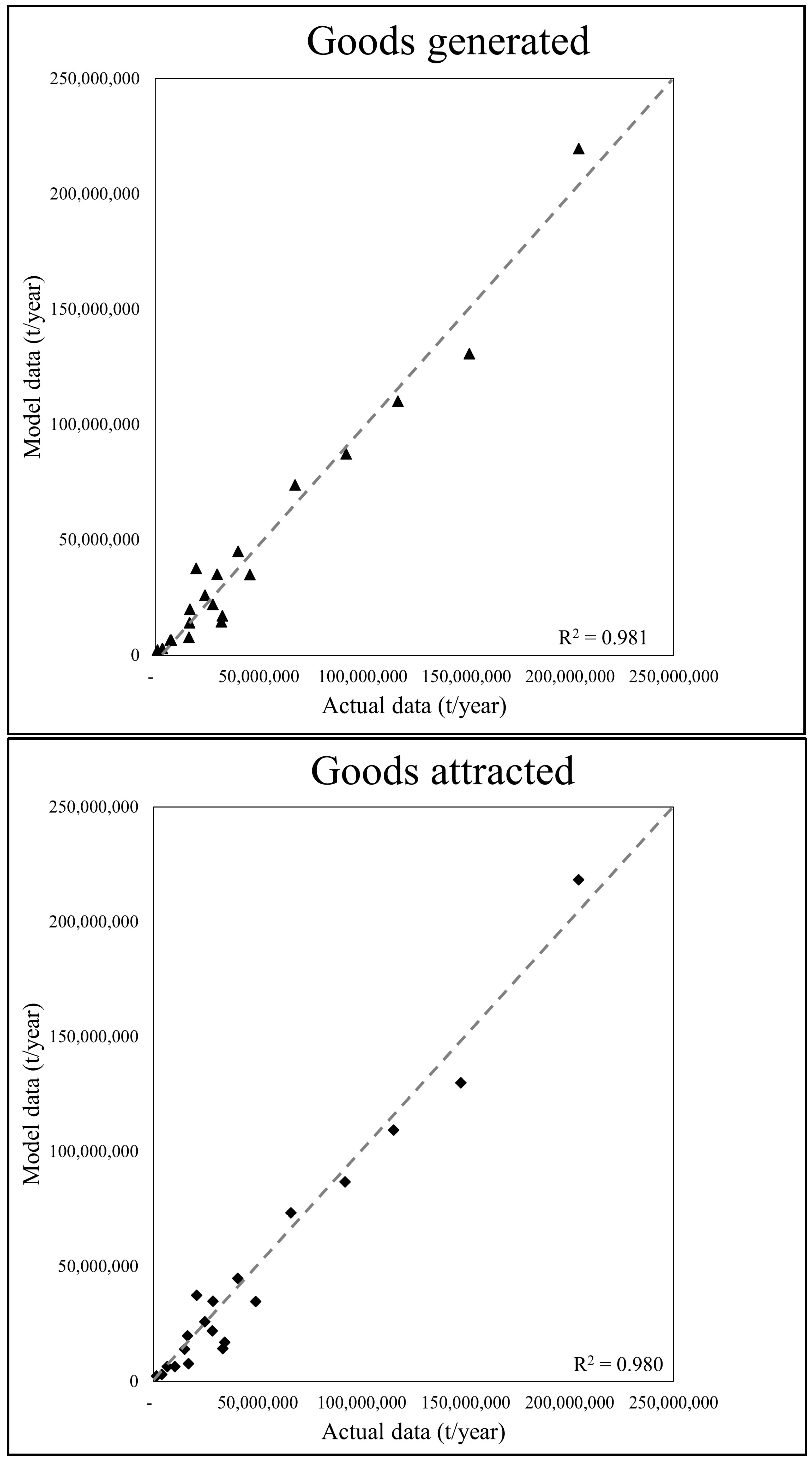
2.1. Regression Models and Estimation of the Matrices

The OD matrices can be estimated starting from the ISTAT road freight transport matrix [30]. This matrix, which refers to the year 2019, provides, in terms of tonnes/year, the goods exchanged by road between the different Italian regions. Similar matrices are not available for smaller territorial aggregations.

OD matrices between smaller areas can be estimated using a model which relates data from the regional ISTAT matrix to other available data [31], such as total employees, employees in the trade sector, employees in the manufacturing sector, resident population, and so on. Different linear regression models were tested, simple and multiple, using one or more variables and correlating them with the total road freight emitted and the total freight attracted by each region. The best results were obtained by correlating both goods generated and attracted with the average number of employees in manufacturing activities. These data are available from ISTAT with a spatial detail down to a single municipality, and therefore, can be used to refine the OD matrix down to the municipal level.

Table 1. Regional data elaborated from the ISTAT database [27,28].

Region	Generated Goods [t/year]	Attracted Goods [t/year]	Employees in Manufacturing Activities
Abruzzo	16,733,577	16,237,471	3439.0
Basilicata	7,294,685	6,552,522	81,727.1
Calabria	7,736,544	10,085,013	9329.9
Campania	39,982,681	40,426,876	24,539.9
Emilia-Romagna	117,100,836	115,411,530	452,620.9
Friuli-Venezia Giulia	24,120,398	24,578,484	106,807.7
Lazio	45,733,494	49,006,578	9182.2
Liguria	31,968,665	33,122,971	59,139.2
Lombardia	204,170,787	204,251,818	903,826.0
Marche	19,834,810	20,630,934	154,771.1
Molise	3,550,801	3,815,597	77,508.7
Piemonte	92,171,837	91,943,760	359,056.0
Puglia	29,949,807	28,541,964	28,952.4
Sardegna	16,348,194	16,737,452	26,000.9
Sicilia	27,832,117	28,222,311	2829.4
Toscana	67,444,868	66,024,129	303,266.1
Trentino Alto Adige	32,391,364	34,206,166	69,942.6
Umbria	16,718,504	14,908,460	57,677.6
Valle d’Aosta	1,117,068	1,374,407	9316.1
Veneto	151,512,857	147,635,451	537,796.5

shows the data used for calibrating the two best linear models, one for estimating ‘generated’ goods (generation index) and the other for estimating ‘attracted’ goods (attraction index).

Table 2. Results and statistical tests.

Results	Generated Goods	Attracted Goods
Coefficient	243.09	241.52
Statistical tests
R2	0.981	0.980
F	≅ 0	≅ 0
t-student	31.04	30.61

reports the resulting statistical tests. The data in this table should be interpreted as follows: the coefficient of determination measures the model’s ability to reproduce the real data and is better closer to 1; the significance test F is valid if it is close to zero; the Student’s t-test verifies whether the variable used is really significant for the reproduction of the phenomenon and, in the case of a single variable, the test is verified if its value is greater than 6.314. All these indicators are valid for calibrated models that are based on the assumption that the linear regression line passes through the origin of the axes. The scatter plots with data concerning actual values and estimated values are reported in Figure 5. The same approach was already tested by the authors in [5] but referred to province-based zoning of the entire Italian territory.

These models enable scaling the regional OD matrix to other matrices based on smaller zones. We assume that the parameter ‘distance between zones’ can be neglected, considering that only long distances, such as those between regions, already implicit in the starting matrix, can influence freight transport.

2.2. National Model

For the national-scale model, the study area was the entire Italian territory. This study area was partitioned into traffic zones (zoning) with the following criteria:

• Campania and its neighbouring regions were partitioned into provincial areas.
• For the other regions, the zones correspond to their territory.
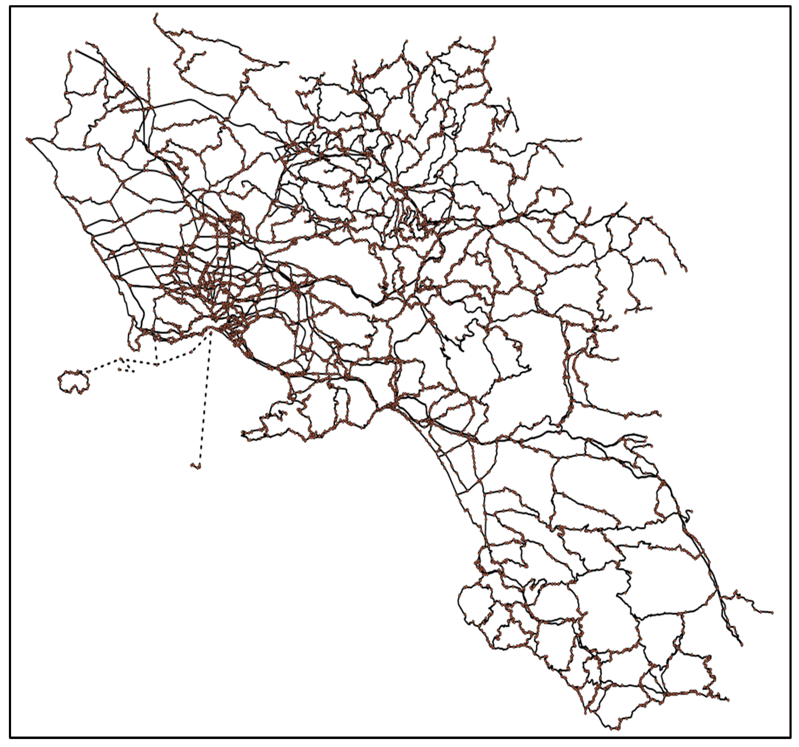
• Overall, the study area was partitioned into 35 zones, as shown in Figure 6.

The transport supply model on the national scale was implemented to be congruent with the corresponding zoning, densifying the road network in the Campania region. The corresponding graph (Figure 7) has 368 links and 256 nodes and represents over 22,000 km of roads; the free-flow speeds considered for heavy goods vehicles (HGVs) are reported in

Table 3. Free-flow speeds for HGVs (national model) [4].

Road Type	Free-Flow Speed (km/h)
Connector	15
Motorway (130)	90
Motorway (90)	70
Rural road (90)	65
Rural road (70)	50
Rural road (50)	35
Sea link	10

.

Once implemented, the supply model estimated the transport demand using generation and attraction indices, a deterministic assignment procedure was applied to calculate freight flows, again in terms of tonnes/year, on the national network; the results are reported in Figure 8 and allow us to estimate the flows of exchange and crossing goods with the Campania region, through the generation of a cordon (boundary of the study area) matrix based on the main roads entering the region. These data are necessary for building the whole regional matrix.

2.3. Regional Model

The regional study area was the territory of the Campania; it was partitioned into 551 zones, equal to the number of municipalities (Figure 9). The cordon sections were 10; therefore, the OD matrix had 314,721 cells (561 × 561). This matrix could be divided into four submatrices (Figure 10):

• Internal trips matrix, or I–I matrix, which reports the trips that have both the origin and destination within the study area;
• Matrix of internal-external exchange trips, or I–E matrix, which reports the trips that have their origin within the study area and their destination outside the study area;
• Matrix of external-internal exchange trips, or E–I matrix, which reports the trips that have their origin outside the study area and their destination within the study area;
• Crossing trips matrix, or E–E matrix, which reports the trips that have both origin and destination outside the study area.

The I–I matrix was estimated according to the number of manufacturing employees, with the same procedure used for the national model. The goods emitted were therefore estimated by distributing the total goods with origin and destination in the Campania region in proportion to the manufacturing employees of each municipality, obtaining the quantity of goods emitted by each municipality. The goods emitted by each municipality were distributed among the destination municipalities in proportion to the number of manufacturing employees in each municipality.

The E–E matrix was directly obtained from the cordon matrix estimated through the assignment procedure on the national model.

The E–I exchange matrix provides the flows of goods entering the study area from each cordon section and destined for the five provinces of the region. The flows destined to each municipality were estimated by dividing the flows destined to each province in proportion to the number of manufacturing employees at the destination. Similarly, the I–E matrix provides the flows of goods originating in the five provinces and exiting the different sections at the border of the study area. The estimated exiting flows from each municipality were obtained by distributing them in proportion to the manufacturing employees at the origin.

This matrix is expressed in terms of tonnes/year of goods; we assumed an average load per vehicle of 9 tonnes, based on data from the National Transport Account [32], and thus estimate the corresponding matrix in terms of vehicles/year. This matrix contains all trips between municipalities. Considering that FCEVs should only be used on long trips, the matrix has been modified by eliminating all trips that occur between municipalities belonging to the same province; all exchange and crossing trips and all trips between different provinces remain.

The regional road network model includes more than 22,000 arcs, representing over 7000 km of roads (Figure 11). The network includes all motorways, state and regional roads and the main provincial and municipal roads in the study area. Each road link has been associated with a free-flow speed (for heavy goods vehicles) summarised in

Table 4. Free-flow speed for HGVs (regional model) [4].

Road Type	Free-Flow Speed (km/h)
Connector	15
Motorway 3 lanes (130)	90
Motorway 2 lanes (130)	90
Motorway 2 lanes (115)	80
Motorway 2 lanes (100)	75
Urban motorway 3 lanes (80)	70
Motorway link 2 lanes (90)	70
Ramp 1 lane (40)	30
National road 2 lanes (90)	65
National road 2 lanes (80)	55
National road 1 lane (70)	50
National road 1 lane (60)	40
National road 1 lane (50)	35
National road 1 lane (40)	30
Provincial road 2 lanes (80)	55
Provincial road 2 lanes (70)	50
Provincial road 2 lanes (60)	40
Provincial road 1 lane (70)	45
Provincial road 1 lane (60)	35
Provincial road 1 lane (50)	30
Provincial road 1 lane (40)	25
Urban road 2 lanes (50)	30
Urban road 1 lane (50)	25
Urban road 1 lane (40)	20
Urban road 1 lane (30)	15

.

Once the regional OD matrix was estimated, in terms of freight vehicles/year, with the transport supply model, we estimated the traffic flows on the network through a deterministic assignment procedure, such as the one already used for the national-scale model. The results of the assignment are shown in Figure 12. The high values, compared to the others, were expected in the exchange and crossing flows. The results in terms of vehicle-km/year are summarised in

Table 5. Estimated vehicle-km/year [4].

Road Type	Vehicle-km/Year (Total)	Vehicle-km/Year (Long-Distance)
Motorway 3 lanes (130)	276,119,152	274,527,847
Motorway 2 lanes (130)	19,733,091	19,178,558
Motorway 2 lanes (115)	95,975,044	95,660,848
Motorway 2 lanes (100)	196,306,520	190,831,397
Urban motorway 3 lanes (80)	7,340,772	5,488,682
Motorway link 2 lanes (90)	38,178,898	37,903,014
Ramp 1 lane (40)	13,498,693	12,285,300
National road 2 lanes (90)	22,633,887	19,135,577
National road 2 lanes (80)	300,130	297,027
National road 1 lane (70)	36,819,806	33,881,080
National road 1 lane (60)	6,329,728	5,946,401
National road 1 lane (50)	13,220,155	12,408,607
National road 1 lane (40)	352,212	251,271
Provincial road 2 lanes (80)	915,896	540,722
Provincial road 2 lanes (70)	92,855	82,478
Provincial road 2 lanes (60)	1,316,643	828,484
Provincial road 1 lane (70)	9,919,839	8,039,685
Provincial road 1 lane (60)	3,453,499	3,032,760
Provincial road 1 lane (50)	5,194,020	4,692,878
Provincial road 1 lane (40)	305,588	288,786
Urban road 2 lanes (50)	4,027,299	3,055,757
Urban road 1 lane (50)	2,959,986	2,160,573
Urban road 1 lane (40)	3,029,699	2,479,922
Urban road 1 lane (30)	497,069	342,547
Total	758,520,481	733,340,201

.

The period on which the analysis of the effects of the introduction of FCEVs for freight transport was focused is between 2025 and 2040. The year 2025 was chosen as the initial year of application of the measure included in the NRRP; in 2030 it was assumed that what was expected in the plan would be realised (market penetration in long-distance freight transport of up to 5–7%) and the analysis was extended to the following 10 years, with different assumptions on the market penetration rate. It was therefore necessary to estimate the trend in freight transport demand for the years after 2019. Data from the Italian Institute for Environmental Protection and Research (ISPRA) [33] on the vehicle-km/year of diesel heavy goods vehicles from 2010 to 2019 were used. An average annual decrease of 1.02% (23.3 billion in 2010, 20.6 billion in 2019) can be noted, which contrasts the growth in overall freight demand, represents the transition already started towards low-emissions alternative fuels, and the trend to use more sustainable alternatives (rail and maritime transport) for long-distance freight transport. Using these data, it is possible to estimate the vehicle-km/year from 2025 to 2040 (

Table 6. Estimated vehicle-km/year on long distances between 2025 and 2040 [4].

Year	Coefficient	Vehicle-km/Year (Long-Distance)
2019	-	733,340,201
-----	------	------
2025	0.939	688,459,783
2026	0.929	680,979,713
2027	0.918	673,499,643
2028	0.908	666,019,572
2029	0.898	658,539,502
2030	0.888	651,059,432
2031	0.878	643,579,362
2032	0.867	636,099,292
2033	0.857	628,619,222
2034	0.847	621,139,152
2035	0.837	613,659,082
2036	0.827	606,179,012
2037	0.816	598,698,942
2038	0.806	591,218,872
2039	0.796	583,738,802
2040	0.786	576,258,732

).

3. Impacts on CO₂ Emissions and Fuel Consumption

The estimated impacts on CO₂ emissions and fuel consumption were obtained considering the following two main assumptions: (a) the hydrogen used is produced exclusively from renewable sources (green hydrogen); (b) the emissions and consumption associated with transporting hydrogen from the place of production to storage locations and refuelling stations are equal to those of conventional fuels. In this case, it can be assumed that the reductions in consumption and emissions are equal to those that would be produced by diesel vehicles being replaced by FCEVs.

Regarding CO₂ emissions, the average factor for heavy goods vehicles proposed by Corinair [34] can be used and is equal to 718.16 g/km. For fuel consumption, on the other hand, a value of 0.244 L/km can be assumed. This value was obtained based on the average consumption in g/km estimated in [34] for different heavy diesel vehicles, the percentage of these in the vehicle fleet and the specific weight of diesel fuel (830 g/L). The data taken from Corinair research are consolidated and updated, also considering changes in the vehicle fleet, and can be considered valid for this work, assuming that the models used are macroscopic and provide aggregated values of annual traffic flows.

We considered three scenarios. All scenarios assume a linear growth of the market penetration rate between 2025 and 2030, starting with a value of 1.2% and arriving at a value of 7.0%, thus with a growth rate of 1.16% per year. From 2030 to 2040, the three scenarios differ in terms of growth rates, as follows:

• A ‘pessimistic’ scenario, where the penetration rate remains equal to 7% (growth rate equal to zero);
• A ‘linear’ scenario, where the annual growth rate is 1.16% (maintaining the trend of the previous 5 years);
• An ‘optimistic’ scenario, where the annual growth rate is 1.5%.

Furthermore, we introduced, for comparison, a baseline scenario (no-FCEV) which projects the current figures to 2040, considering that no FCEV development occurs; this scenario also shows a reduction in emissions due to the trend shown in Table 6.

Table 7. Estimated CO₂ emission reduction, w.r.t. 2019 [4].

Year	No-FCEV Scenario [t/Year]	Pessimistic Scenario [t/Year]	Linear Scenario [t/Year]	Optimistic Scenario [t/Year]
2025	32,230	38,163	38,163	38,163
2026	37,602	49,143	49,143	49,143
2027	42,974	59,998	59,998	59,998
2028	48,345	70,729	70,729	70,729
2029	53,717	81,335	81,335	81,335
2030	59,089	91,817	91,817	91,817
2031	64,460	96,813	102,174	103,745
2032	69,832	101,808	112,406	115,512
2033	75,204	106,804	122,514	127,118
2034	80,575	111,800	132,497	138,563
2035	85,947	116,795	142,355	149,847
2036	91,319	121,791	152,089	160,970
2037	96,690	126,787	161,698	171,931
2038	102,062	131,782	171,183	182,731
2039	107,434	136,778	180,543	193,370
2040	112,805	141,774	189,778	203,848

reports the estimated reductions in CO₂ emissions, compared to 2019, for the four scenarios, while

Table 8. Total CO₂ emission reduction, w.r.t. no-FCEV scenario [4].

Year	Pessimistic Scenario [t/Year]	Linear Scenario [t/Year]	Optimistic Scenario [t/Year]
2025	5933	5933	5933
2026	11,541	11,541	11,541
2027	17,025	17,025	17,025
2028	22,384	22,384	22,384
2029	27,618	27,618	27,618
2030	32,728	32,728	32,728
2031	32,352	37,714	39,285
2032	31,976	42,574	45,680
2033	31,600	47,310	51,915
2034	31,224	51,921	57,988
2035	30,848	56,408	63,900
2036	30,472	60,770	69,651
2037	30,096	65,008	75,241
2038	29,720	69,121	80,669
2039	29,344	73,109	85,937
2040	28,968	76,973	91,043
Total	423,832	698,138	778,538

shows the differential reductions compared to the baseline scenario (no-FCEV). Overall, the emissions saved over the reference period vary between 423,832 and 778,538. Compared with the no-FCEV scenario the amount of the reductions in percentages varies from 5.83% to 10.71%.

The fuel savings in each year of the time horizon and for the assumed scenarios are summarised in

Table 9. Total fuel savings, w.r.t. no-FCEV scenario.

Year	Pessimistic Scenario [L/Year]	Linear Scenario [L/Year]	Optimistic Scenario [L/Year]
2025	2,016,190	2,016,190	2,016,190
2026	3,922,092	3,922,092	3,922,092
2027	5,785,643	5,785,643	5,785,643
2028	7,606,843	7,606,843	7,606,843
2029	9,385,692	9,385,692	9,385,692
2030	11,122,189	11,122,189	11,122,189
2031	10,994,406	12,816,336	13,350,350
2032	10,866,622	14,468,131	15,523,746
2033	10,738,838	16,077,575	17,642,377
2034	10,611,055	17,644,668	19,706,244
2035	10,483,271	19,169,410	21,715,347
2036	10,355,487	20,651,800	23,669,685
2037	10,227,704	22,091,840	25,569,259
2038	10,099,920	23,489,528	27,414,068
2039	9,972,136	24,844,865	29,204,113
2040	9,844,353	26,157,851	30,939,394
Total	144,032,440	237,250,653	264,573,232

, compared to the no-FCEV scenario. The total savings over the period range from 144 to 264 million litres of diesel.

4. Conclusions

The use of hydrogen for automotive purposes can significantly contribute to combating global warming. The use of electrically powered vehicles is one of the main strategies for promoting sustainable mobility [35], especially from the perspective of increasing shares of energy produced from renewable sources. The promotion of the use of fuel cell electric vehicles for the freight transport sector has been identified in Italy, within the framework of the NRRP, as a valid strategy for encouraging the ecological transition.

This study has proposed a methodology and applied it to a regional context to estimate the impacts on consumption and greenhouse gas emissions of the development of FCEVs for long-distance freight transport. The savings in both consumption and emissions are significant in percentage terms, compared to the status quo scenario and vary, depending on different assumptions of growth in the use of these vehicles, between 5.83% and 10.71%. Specifically, CO₂ emissions are reduced by between 423,832 and 778,538 tonnes, and diesel consumption is reduced by between 144 and 264 million litres, within the reference time horizon (2025–2040).

The analysis only covered freight transport; however, a positive effect can also be expected on passenger transport due to the spread of refuelling stations. It is believed, however, that the spread of FCEV cars is only possible with a capillary diffusion of refuelling stations, also in urban areas.

Another important point concerns the production of hydrogen. Ji and Wang [36] studied and compared hydrogen production methods and pointed out that a considerable portion is still obtained from fossil sources (mainly, steam methane reforming, oil reforming and coal gasification); therefore, to date, most hydrogen is produced from non-renewable sources and with CO₂ emissions. Even the production of green hydrogen [37] is not entirely emissions-free. Given that the calculations are based on replacing diesel-powered vehicles with hydrogen-powered vehicles, the CO₂ emission savings are ‘at the tailpipe’. Although it can be assumed that there is an offset, even favourable to our hypothesis, between the CO₂ used to produce the diesel fuel and that to produce the green hydrogen, just as the emissions associated with the distribution of the two fuel types can be considered more or less equivalent, if the green hydrogen hypothesis were to be removed, the estimated CO₂ savings would be significantly overestimated, although the positive effects on other pollutant emissions and fuel savings would remain. Therefore, without investment policies aimed at producing green hydrogen in Italy, any action to promote FCEVs may have positive effects on air pollution and consumption, but not on climate-changing emissions.

Research prospects may be directed toward assessing the impacts related to the diffusion of this technology to private cars, at analysing other territorial contexts, e.g., of other European countries, and at optimising the location of refuelling stations, which are certainly a critical aspect to enable the widespread use of this technology.

Regarding this last point, the simulation model developed in this paper could be very useful for identifying the optimal locations, which are the those which can intercept as many vehicles as possible.

References

1. European Commission, Next Generation EU: Next Steps for RRF. 2020. Available online: https://ec.europa.eu/commission/presscorner/detail/en/IP_20_1658 (accessed on 18 February 2022).
2. Italia Domani, Piano Nazionale di Ripresa e Resilienza. 2021. Available online: https://www.governo.it/sites/governo.it/files/PNRR.pdf (accessed on 18 February 2022).
3. European Commission. The Role of Hydrogen in Meeting Our 2030 Climate and Energy Targets. Available online: https://ec.europa.eu/commission/presscorner/detail/en/fs_21_3676 (accessed on 13 October 2022).
4. Gallo, M.; Marinelli, M. The Impact of Fuel Cell Electric Vehicles for Freight Transport on CO2 Emissions: A Case Study. In Proceedings of the 2022 IEEE International Conference on Environment and Electrical Engineering and 2022 IEEE Industrial and Commercial Power Systems Europe (EEEIC/I&CPS Europe), Prague, Czech Republic, 28 June 2022–1 July 2022; pp. 1–6. [Google Scholar] [CrossRef]
5. Gallo, M.; Marinelli, M. The impact of fuel cell electric freight vehicles on fuel consumption and CO2 emissions: The case study of Italy. Sustainability 2022, 14, 13455. [Google Scholar] [CrossRef]
6. Cunanan, C.; Tran, M.-K.; Lee, Y.; Kwok, S.; Leung, V.; Fowler, M. A Review of Heavy-Duty Vehicle Powertrain Technologies: Diesel Engine Vehicles, Battery Electric Vehicles, and Hydrogen Fuel Cell Electric Vehicles. Clean Technol. 2021, 3, 474–489. [Google Scholar] [CrossRef]
7. European Automobile Manufacturers Association. ACEA Report Vehicles in Use Europe 2019. Available online: https://www.acea.auto/uploads/publications/ACEA_Report_Vehicles_in_use-Europe_2019.pdf (accessed on 15 December 2021).
8. International Energy Association. The Future of Trucks Implications for Energy and the Environment. 2017. Available online: https://www.oecd.org/publications/the-future-of-trucks-9789264279452-en.htm (accessed on 15 December 2021).
9. European Environment Agency. Carbon Dioxide Emissions from Europe’s Heavy-Duty Vehicles. 2020. Available online: https://www.eea.europa.eu/themes/transport/heavy-duty-vehicles (accessed on 15 December 2021).
10. Elgowainy, A.; Rousseau, A.; Wang, M.; Ruth, M.; Andress, D.; Ward, J.; Joseck, F.; Nguyen, T.; Das, S. Cost of ownership and well-to-wheels carbon emissions/oil use of alternative fuels and advanced light-duty vehicle technologies. Energy Sustain. Dev. 2013, 17, 626–641. [Google Scholar] [CrossRef]
11. Selmi, T.; Khadhraoui, A.; Cherif, A. Fuel cell–based electric vehicles technologies and challenges. Environ. Sci. Pollut. Res. 2022, 29, 78121–78131. [Google Scholar] [CrossRef] [PubMed]
12. Dash, S.K.; Chakraborty, S.; Roccotelli, M.; Sahu, U.K. Hydrogen Fuel for Future Mobility: Challenges and Future Aspects. Sustainability 2022, 14, 8285. [Google Scholar] [CrossRef]
13. Wanniarachchi, S.; Hewage, K.; Wirasinghe, C.; Chhipi-Shrestha, G.; Karunathilake, H.; Sadiq, R. Transforming road freight transportation from fossils to hydrogen: Opportunities and challenges. Int. J. Sustain. Transp. 2022, 1–21. [Google Scholar] [CrossRef]
14. Alvarez-Meaza, I.; Zarrabeitia-Bilbao, E.; Rio-Belver, R.M.; Garechana-Anacabe, G. Fuel-Cell Electric Vehicles: Plotting a Scientific and Technological Knowledge Map. Sustainability 2020, 12, 2334. [Google Scholar] [CrossRef] [Green Version]
15. International Energy Agency. Advanced Fuel Cells Technology Collaboration Programme. Report on Mobile Fuel Cell Application: Tracking Market Trends. Available online: https://www.ieafuelcell.com/fileadmin/publications/2020_AFCTCP_Mobile_FC_Application_Tracking_Market_Trends_2020.pdf (accessed on 13 December 2022).
16. Rinawati, D.I.; Keeley, A.R.; Takeda, S.; Managi, S. A systematic review of life cycle assessment of hydrogen for road transport use. Prog. Energy 2022, 4, 012001. [Google Scholar] [CrossRef]
17. Breuer, J.L.; Samsun, R.C.; Stolten, D.; Peters, R. How to reduce the greenhouse gas emissions and air pollution caused by light and heavy duty vehicles with battery-electric, fuel cell-electric and catenary trucks. Environ. Int. 2021, 152, 106474. [Google Scholar] [CrossRef]
18. Carrara, S.; Longden, T. Freight futures: The potential impact of road freight on climate policy. Transp. Res. D 2017, 55, 359–372. [Google Scholar] [CrossRef] [Green Version]
19. Gonzalez Palencia, J.C.; Araki, M.; Shiga, S. Energy consumption and CO2 emissions reduction potential of electric-drive vehicle diffusion in a road freight vehicle fleet. Energy Procedia 2017, 142, 2936–2941. [Google Scholar] [CrossRef]
20. Moriarty, P.; Honnery, D. Prospects for hydrogen as a transport fuel. Int. J. Hydrog. Energy 2019, 44, 16029–16037. [Google Scholar] [CrossRef]
21. Forrest, K.; Kinnon, M.M.; Tarroja, B.; Samuelsen, S. Estimating the technical feasibility of fuel cell and battery electric vehicles for the medium and heavy duty sectors in California. Appl. Energy 2020, 276, 115439. [Google Scholar] [CrossRef]
22. Nugroho, R.; Rose, P.K.; Gnann, T.; Wei, M. Cost of a potential hydrogen-refueling network for heavy-duty vehicles with long-haul application in Germany 2050. Int. J. Hydrog. Energy 2021, 46, 35459–35478. [Google Scholar] [CrossRef]
23. Noll, B.; del Val, S.; Schmidt, T.S.; Steffen, B. Analyzing the competitiveness of low-carbon drive-technologies in road-freight: A total cost of ownership analysis in Europe. Appl. Energy 2022, 306, 118079. [Google Scholar] [CrossRef]
24. Yan, J.; Zhao, J. Willingness to pay for heavy-duty hydrogen fuel cell trucks and factors affecting the purchase choices in China. Int. J. Hydrog. Energy 2022, 47, 24619–24634. [Google Scholar]
25. Yan, J.; Wang, G.; Chen, S.; Zhang, H.; Qian, J.; Mao, Y. Harnessing freight platforms to promote the penetration of long-haul heavy-duty hydrogen fuel-cell trucks. Energy 2022, 254, 124225. [Google Scholar] [CrossRef]
26. de las Nieves Camacho, M.; Jurburg, D.; Tanco, M. Hydrogen fuel cell heavy-duty trucks: Review of main research topics. Int. J. Hydrog. Energy 2022, 47, 29505–29525. [Google Scholar] [CrossRef]
27. Liu, F.; Maurezall, D.L.; Zhao, F.; Hao, H. Deployment of fuel cell vehicles in China: Greenhouse gas emission reductions from converting the heavy-duty truck fleet from diesel and natural gas to hydrogen. Int. J. Hydrog. Energy 2021, 46, 17982–17997. [Google Scholar] [CrossRef]
28. Çabukoglu, E.; Georges, G.; Küng, L.; Pareschi, G.; Boulouchos, K. Fuel cell electric vehicles: An option to decarbonize heavy-duty transport? Results from a Swiss case-study. Transp. Res. D 2019, 70, 35–48. [Google Scholar] [CrossRef]
29. Vijayakumar, V.; Jenn, A.; Fulton, L. Low carbon scenario analysis of a hydrogen-based energy transition for on-road transportation in California. Energies 2021, 14, 7163. [Google Scholar] [CrossRef]
30. ISTAT, Matrice Trasporto Merci su Strada 2019. Available online: http://dati.istat.it/ (accessed on 18 December 2021).
31. ISTAT, Imprese e Addetti. Available online: http://dati.istat.it/Index.aspx?DataSetCode=DICA_ASIAUE1P (accessed on 18 December 2021).
32. Conto Nazionale Delle Infrastrutture e dei Trasporti. Anni 2018–2019; Istituto Poligrafico Zecca dello Stato: Rome, Italy, 2021.
33. ISPRA, Serie Storiche Delle Emissioni Nazionali di Inquinanti Atmosferici 1990–2019. Available online: http://emissioni.sina.isprambiente.it/serie-storiche-emissioni/ (accessed on 18 February 2022).
34. EMEP/EEA. Air Pollutant Emission Inventory Guidebook 2019—Part B—1.A.3.b.i–iv Road Transport 2019. Available online: https://www.eea.europa.eu/publications/emep-eea-guidebook-2019/part-b-sectoral-guidance-chapters/1-energy/1-a-combustion/1-a-3-b-i/view (accessed on 7 September 2022).
35. Gallo, M.; Marinelli, M. Sustainable Mobility: A Review of Possible Actions and Policies. Sustainability 2020, 12, 7499. [Google Scholar] [CrossRef]
36. Ji, M.; Wang, J. Review and comparison of various hydrogen production methods based on costs and life cycle impact assessment indicators. Int. J. Hydrog. Energy 2021, 46, 38612–38635. [Google Scholar] [CrossRef]
37. Xu, X.; Zhou, Q.; Yu, D. The future of hydrogen energy: Bio-hydrogen production technology. Int. J. Hydrog. Energy 2022, 79, 33677–33698. [Google Scholar] [CrossRef]
Figure 1. A configuration scheme of the main FCEV powertrain components.
Energies 16 00508 g001
Figure 2. Procedure—Phase 1: national OD matrix and regional OD internal matrix.
Energies 16 00508 g002
Figure 3. Procedure—Phase 2: regional OD total matrix.
Energies 16 00508 g003
Figure 4. Procedure—Phase 3: vehicle-km/year and savings estimation.
Energies 16 00508 g004
Figure 5. Comparison between model data and actual data.
Energies 16 00508 g005
Figure 6. Study area and zoning (national model).
Energies 16 00508 g006
Figure 7. Road network (national model).
Energies 16 00508 g007
Figure 8. Freight road flows (national model).
Energies 16 00508 g008
Figure 9. Study area and zoning (regional model).
Energies 16 00508 g009
Figure 10. OD matrix scheme.
Energies 16 00508 g010
Figure 11. Road network (regional model).
Energies 16 00508 g011
Figure 12. Estimated traffic flows (regional model).
Energies 16 00508 g012