Article

Analysis of the Behavior Pattern of Energy Consumption through Online Clustering Techniques

by
Juan Viera
1,
Jose Aguilar
1,2,3,4,*,
Maria Rodríguez-Moreno
1,5 and
Carlos Quintero-Gull
6
1
Escuela Politécnica Superior, ISG—Intelligent Systems Group, Universidad de Alcalá, 28805 Alcalá de Henares, Spain
2
CEMISID—Centro de Estudios en Microprocesadores y Sistemas Digitales, Universidad de Los Andes, Mérida 5101, Venezuela
3
GIDITIC—Grupo de Investigación, Desarrollo e Innovación en Tecnologías de la Información y las Comunicaciones, Universidad EAFIT, Medellín 50022, Colombia
4
IMDEA Networks Institute, Leganés, 28918 Madrid, Spain
5
TNO, Intelligent Autonomous Systems Group (IAS), 2597 AK The Hague, The Netherlands
6
Departamento de Ciencias Aplicadas y Humanísticas, Universidad de Los Andes, Mérida 5101, Venezuela
*
Author to whom correspondence should be addressed.
Energies 2023, 16(4), 1649; https://doi.org/10.3390/en16041649
Submission received: 29 December 2022 / Revised: 1 February 2023 / Accepted: 3 February 2023 / Published: 7 February 2023

Abstract

:
Analyzing energy consumption is currently of great interest to define efficient energy management strategies. In particular, studying the evolution of the behavior of the consumption pattern can allow energy policies to be defined according to the time of the year. In this sense, this work proposes to study the evolution of energy behavior patterns using online clustering techniques. In particular, the centroids of the groups constructed by the techniques will represent their consumption patterns. Specifically, two unsupervised online machine learning techniques ideal for the stated objective will be analyzed, X-Means and LAMDA, since they are capable of varying and adapting the number of clusters at runtime. These techniques are applied to energy consumption data in commercial buildings, making groupings on previous groups, in our case, monthly and quarterly. We compared their performance by analyzing the evolution of the patterns over time. The results are very promising since the quality of the consumption patterns obtained is very good according to the performance metrics. Thus, the three main contributions of this article are to propose an approach to determine energy consumption patterns using online non-supervised learning approaches, a methodology to analyze and explain the evolution of energy consumption using centroids of clusters, and a comparison strategy of online learning techniques. The online clustering techniques have qualities of the order of 0.59 and 0.41 for Silhouette and Davies-Boulding, respectively, for X-Means and of the order of 0.71 and 0.24 for Silhouette and Davies-Boulding, respectively, for LAMDA in different datasets of energy. The results are motivating since very good results are obtained in terms of the quality of the clusters, particularly with LAMDA; therefore, analyzing its centroids as the patterns of user behaviors makes a lot of sense.

1. Introduction

Currently, there is an immense global demand for energy, which is necessary for the functional consumption of most tasks of life, such as lighting, the use of computer equipment, household appliances, and other electronic devices. The aforementioned devices are currently vital in our society. On the other hand, currently, different types of buildings (residential, commercial, and industrial, among others) are being equipped with intelligent devices, such as cameras, sensors, and different actuators [1]. These devices, together with the communication infrastructure, characterize the Internet of Things (IoT) paradigm [2].
Due to the increase in energy required by this paradigm, consumption in homes has increased between 1232 and 1460 kWh per year [3]. It is estimated that the energy consumption derived from this increase in devices will increase much more in the coming years. For example, in Europe, it will go from 4 TWh in 2015 to 104 TWh in 2025 [3]. Due to this increase in energy demand, there is a great concern to achieve greater efficiency and optimization of consumption [1,4,5]. To do this, among other things, it is necessary to identify the consumption pattern of users and, based on that information, propose strategies and mechanisms to save energy resources as much as possible. In the next two sections, we compare other related works and describe the contributions of this paper. Particularly, being able to know how the customer’s energy consumption pattern evolves can be useful in different energy management tasks [6], for example, in the case of providers, to determine when there are more or fewer demands to adjust their offer and, in the case of the client, to know their peaks and from there look for an energy optimization mechanism.

1.1. Related Work

Based on the interest of this article, which is to develop methods that allow the identification of how the pattern of energy consumption of a client evolves, in this section, we will describe those recent works close to this topic. Particularly, since we have not found any work on this specific aspect, we present recent works linked to related topics, specifically on the prediction and optimization of energy consumption.
In general, the current applications of artificial intelligence, and specifically machine learning algorithms, in the field of energy are enormous [6,7,8]. However, there are no recent works on the study of behavioral patterns of energy consumption. Most of the research works on the study of energy consumption and its characteristics focus on reducing consumption and optimizing the use of energy resources using, for example, optimization and predictive models. For example, in [8], Yoon et al. focus on the efficient use of energy and its infrastructure in smart cities using machine learning techniques. The authors use machine learning to create a deep learning network in a smart city to analyze and predict the energy consumption of IoT sensor devices. Wu et al. [9] use ML models to predict the consumption of an intelligent building with the aim of energy conservation and environmental protection.
Xiao et al. [10] carried out a comparison of different configuration parameters for energy models. They propose 2 scenarios, one with only data to predict energy efficiency and another that considers information from spindle motor aging and tool wear. For both cases, they used support vector regression models [11], artificial neural networks [12], and Gaussian process regression [13]. In the article [14], the authors proposed a predictive model based on the energy consumption of the users, which allows the monitoring and estimating of the energy consumption. In this case, they make use of the K-means algorithm and support vector machines.
Other articles that analyze energy consumption, study strategies, and make predictions about energy consumption, among other things, are presented in [15] (based on support vector regression, [16] (based on artificial neural networks), and [17] (based on random forests). In addition, for an analysis of user trends, there are currently various algorithms and methods, as well as techniques, to reduce the complexity of the problem [9,10,18,19,20]. As we can see in this section and to our knowledge, there are no previous works in the literature dedicated to studying the evolution of energy consumption patterns. Most of the works are dedicated to predicting energetic behavior and to diagnosing what may happen in an energetic infrastructure, but none of them have focused on defining energy consumption patterns and monitoring their evolution, and from there, proposing strategies of analysis and the explainability of these patterns.

1.2. Contributions of the Paper

The objective of this work is to identify and analyze the behavior pattern of customers according to their energy consumption profiles. In particular, it is necessary to identify how the pattern of customer behavior changes over time. We propose to use online unsupervised machine learning algorithms to follow/analyze the evolution of energy consumption patterns. For this, we assume that the centroids of the groups obtained by the clustering techniques represent the energy consumption patterns of the group. The main contributions of the work are as follows:
  • We propose a framework to analyze the evolution of energy consumption patterns;
  • We adjust two clustering techniques to carry out an online clustering process of energy consumption data.
The work is organized as follows. Section 2 presents the unsupervised machine learning used in this work. Section 3 describes the experiments and carries out an analysis of the clusters obtained. Section 4 presents an analysis of the evolution of the patterns and a general comparison in different datasets. Finally, the last section presents the conclusions and future work.

2. Online Unsupervised Machine Learning Used

Unsupervised learning algorithms assume that the data is not labeled, and they analyze datasets to identify similarities between the data (similar data make up a cluster) [21]. This paradigm is useful when the categories of the data are not defined and one of the techniques used in this area is clustering algorithms [22]. The main purpose of a clustering algorithm is to separate the data into smaller subsets, called groups (clusters), such that the content of the data is similar in each cluster but different from the content of the other groups. The centroid of a cluster can be understood as its pattern. Particularly, we will use unsupervised online learning to adapt the cluster to changes in user consumption patterns, enabling real-time updates [23]. In this work, we will use X-means and the LAMDA algorithms.

2.1. X-Means

The X-means algorithm is based on K-Means. The K-means algorithm is one of the simplest and most common algorithms used in clustering, dividing the dataset into K clusters. K-means tries to find the center of each cluster, which is representative of a data region [21]. This point is called the centroid. Thus, K-means is a clustering technique based on centroids [22]. K-means alternates between two steps:
  • Assignment of points/individuals to the nearest centroid;
  • Calculation of centroids.
These steps are repeated in a loop until the centroids stabilize.
Particularly, in this work, we will use X-Means, which is an extension of K-Means that allows for varying the value of K (it does not have to be predefined at the beginning, as it happens with K-Means) [24]. Thus, X-means is an incremental sequential K-means that determines the value of K (clusters) based on a function f(K), which is defined by the following Equation [25]:
f K = 1 i f K = 1 S K α K S K 1 i f S k 1 0 , K > 1 1 i f S k 1 = 0 , K > 1
where
α K = 1 3 4 N d i f K = 2 N d > 1 α K 1 + 1 α K 1 6 i f K > 2 N d > 1
where S k is the sum of the cluster distortions when the number of clusters is K (see below), and N d is the number of attributes in the dataset. The term α k S k 1 in the Equation above is an estimate of S k based on S k 1 , made under the assumption that the data have a uniform distribution. The value of f(K) is the ratio of the actual distortion to the estimated distortion and is close to 1 when the data distribution is uniform. When there are areas of concentration in the data distribution, then S k will be less than the estimated value, so f(K) decreases. The smaller f(K), the more concentrated the data distribution. Therefore, values of K that produce a small value of f(K) can be considered to provide well-defined groups.
On the other hand, the distortion of a cluster is the distance between the objects/individuals of a cluster and its centroid, according to the following Equation [25]:
I j = t = 1 N j d x j t , w j 2
where I j is the distortion of the cluster j, w j is the centroid of the cluster j, N j is the number of objects belonging to the cluster j, x j t is the object t belonging to the cluster j, and d( x j t , w j ) is the distance between the object x j t and the centroid w j of the cluster j. Each cluster is represented by its distortion, and the overall impact of all clusters on the entire data set is evaluated by the sum of all distortions, S K , given by the following Equation [25]:
S K = j = 1 K I j
where K is the number of clusters. The number of clusters K is assumed to be much smaller than the number of objects N. In particular, if for any immediate K f(K) shows special behavior, in particular a minimum point, then the value of K should be taken as the number desired of the clusters. Thus, X-Means converges when it obtains a minimum value of f(K).
In this way, X-means determines if new centroids should appear within a current model (Mj). The appearance of new centroids is carried out by dividing some clusters into two, which have been classified as optimizable according to the Schwarz criterion (it is a criterion for the selection of models among a finite set of models) based on the BIC value, defined by the following equation [24]:
B I C M j = l ^ j D p j 2 . l o g R
where l ^ j D is the logarithmic probability of the data in the model Mj; p j is the number of free parameters present in the model Mj; and R represents the number of samples present in D (R = |D|).
In essence, X-means starts with a given K, goes on to add centroids (changes the K) according to the value of f(K), and calculates the BIC score for each cluster to determine, if any, which cluster to split. When X-Means converges (determines the ideal value of K for that data set), then the final clustering is obtained.

2.2. LAMDA (Learning Algorithm for Multivariate Data Analysis)

LAMDA is a non-iterative fuzzy algorithm based on the degree of adequacy of an individual (data) to a group. It provides great versatility since it allows users to not specify the number of clusters during the execution, and furthermore, it can work online [26,27]. LAMDA works by performing an evaluation of the similarity between the descriptors of an element X of the form X = { x 1 , x 2 , . . . , x j , . . . x m } , which is its vector with m descriptors, with the descriptors of the centroids of the existing clusters, to define in which cluster this data X should be entered. In addition, once X has been assigned to a cluster, it becomes X = { x 1 , x 2 , . . . , x j , . . . x m , c i } , i = 1, 2, … k, where c i is the label associated with X [26]. The base definitions of LAMDA are summarized below [7,26].
Normalization. Each descriptor of X must be normalized based on its maximum and minimum values:
x j = x j x j m i n x j m a x x j m i n
where ( x j ) is the normalized value of descriptor j, x j m i n is the minimum value of descriptor j, and x j m a x is the maximum descriptor of descriptor j. The element resulting from normalization X will be used to compute the degree of adequacy of the element to each existing cluster.
The Degree of Marginal Adequacy (MAD) determines the degree of similarity of a descriptor with respect to another descriptor in a given class. For the calculation of the MAD, density functions are used; the most common is the fuzzy binomial function:
M A D ( x j / ρ k j ) = ρ k j x j ( 1 ρ k j ) ( 1 x j )
where ρ k j is the mean value of descriptor j in the cluster k, calculated by:
ρ k j = 1 n k j t = 1 n k j x j ( t )
where ρ k j is progressively updated each time a new element is added to the cluster.
The function for M A D ( x j / ρ k j ) is the density function of the binomial distribution, which can be interpreted as the probability that the analyzed normalized descriptor belongs to a cluster j, given its mean ρ k j .
The Degree of Global Adequacy (GAD) determines the degree of adequacy of a sample to each existing cluster; it is calculated by mixing the MAD with aggregation functions. These functions are interpolations between the t-norm (T) and the t-conorm (S) like the Dombi operator [28]:
T ( a , b ) = 1 1 + ( 1 a a ) p + ( 1 b b ) p p
S ( a , b ) = 1 1 1 + ( 1 a a ) p + ( 1 b b ) p p
In most cases, p = 1 is used to obtain an approximation close to a linear behavior of the t-norm and the t-conorm [28].
There is also a requirement parameter, 0 < α < 1, used to calibrate fuzzy partitioning data [29]. If α = 1, then GAD is calculated as the t-norm, obtaining a stricter clustering. If α = 0, then GAD is computed as a t-conorm, leading to a more permissive grouping. Thus, α produces a linear interpolation between the t-norm and the t-conorm to calculate the GAD [30].
G A D X , k M A D k , 1 , . . . , M A D k , 1 = α T ( M A D k , 1 , . . . , M A D k , 1 ) + ( 1 α ) S ( M A D k , 1 , . . . , M A D k , 1 )
On the other hand, when an individual (data) does not belong to any class, then a non-informative class (NIC) is created, which will be a new cluster. The GAD of the data entering the NIC is computed considering that M A D N I C j = 0.5 , independent of the value of x j :
G A D X , N I C = α T ( 0.5 , . . . , 0.5 ) + ( 1 α ) S ( 0.5 , . . . , 0.5 )
That element that enters the NIC becomes the first element of the new cluster.
Finally, the assignment of elements to a cluster is done by calculating the maximum GAD of all classes. The index (in) corresponds to the number of the class where the element will be assigned:
in = max   ( G A D 1 X , G A D k X , . . . , G A D m X , G A D N I C X )

3. Experiments

In this section, we will explain how we performed the instantiation and execution of the two techniques presented in the previous section.

3.1. Data Preparation

For this experiment, we used a real dataset from [31]. The first task was to divide the dataset into several files by time periods. In our case, they were divided by months or quarters. From the original data, more data was generated using the distribution of each variable in the dataset in order to increase the amount of data for our execution.
This first dataset corresponded to data taken from a commercial building in 2018. The building had a maximum hourly consumption of 48 W/m2, and the annual consumption was 183.2 kWh/m2 [31]. Each variable in the dataset was taken every half hour throughout the year, breaking down the total consumption in kW as follows: total consumption, light, heat pump, air treatment units, circulation pumps, heating and hot water, cooling, air coolers, and elevators.

3.2. Metrics

To evaluate the quality of the online clustering algorithms, we used two metrics: an ideal metric for distance-based algorithms like X Means (Silhouette coefficient [32]) and another metric for density-based algorithms (Davies-Bouldin index [33]).

3.2.1. Silhouette

The silhouette coefficient is a measure of the cohesion of the clusters. It determines the degree of similarity between the objects of the same cluster [32]. To get this measurement, the average of the proximities between its elements is calculated. This metric is therefore effective in situations where the clusters have a circular shape [23,32] or are grouped around a point. The silhouette coefficient for a data sample is determined with the mean of the silhouette coefficient for each sample data, calculated as [32]:
S S = i = 1 n b i a ( i ) max { a i , b i }
where a(i) and b(i) are computed for each sample i of the cluster C i ( i C i ) for a i = ( C i 1 ) 1 j C i , i j d ( i , j ) and b i = m i n k i | C k | 1 j C k d ( i , j ) , where d(i, j) is the distance between the points i and j.
The coefficient gives a result between −1 and 1. Values close to 1 are the most optimal, those close to 0 indicate that there are overlapping clusters, and negative values generally indicate that there are samples erroneously assigned to clusters. As a general rule, the higher the silhouette coefficient, the better defined the clusters will be [23].

3.2.2. Davies-Bouldin

The Davies-Bouldin index is defined as the mean similarity of each cluster with its most similar cluster. This measure compares the distance between both clusters with the size of the clusters themselves [33]. The measure can be used to infer the adequacy of a data partition. The Davies-Bouldin index is calculated as [33]:
S D B = 1 k i = 1 k max i j R i j
where R i j is the similarity between the clusters i and j. There are different ways to calculate R i j , one of them is R i j = s i + s j d i j , where s i is the average distance between each point of cluster i and the center of cluster i, and d(i, j) is the distance between the centroids of the clusters i and j.
The minimum value that can be obtained using this index is 0, which is the case when there are as many clusters as there are individuals. Therefore, it is understood that the best values of this metric are those closest to 0 since they indicate a better partition and a model with better separation between clusters [23,33].

3.3. Modeling

Next, we proceed to describe how the clustering models are obtained with each algorithm, using a time period (iteration) of a month.

3.3.1. X-Means

In the first iteration, k is initialized to 3 (number of initial clusters), a value that X-Means then optimizes in that first iteration (month). In the following iterations (months), the algorithm readjusts that value of K. In the specific case of the dataset used, the X-Means determined that 20 clusters were necessary on its second iteration. This number of clusters was maintained throughout the 12 months; the X-Means determined that it is the ideal value of K in each iteration (month).
We started by evaluating the centroids of the 20 clusters from January to December in Figure 1 and Figure 2. The centroids for the analysis were normalized between 0 and 1 to graph them (it is the X-axis of Figure 1, Figure 2, Figure 3, Figure 4 and Figure 5), and then the energy consumption represented by them was what we analyzed next. Looking at both figures, it can be seen that in a range of approximately 0.14 and 0.06 in the centroids (equivalent to a range between 200 kW and 400 kW over the total of kW), there were 10 clusters. We also saw 2 clusters in the upper range of Figure 2, which stood out for being separated from those in the middle zone. Clusters 19 and 20 were isolated from the rest throughout the run, slightly converging and stabilizing at the end of the run. Particularly, in Figure 2, we saw that in the summer months, clusters 19 and 20 behaved erratically; perhaps with a greater number of clusters, this behavior would be softened.
In this particular case, clusters 19 and 20 represented a high consumption; in one case, the consumption was higher due to the circulation pumps, and in the other case, it was due to the heat pump and heating and hot water. Finally, cluster 5 represented the pattern with the lowest consumption (around 250 kW), which was generated by several variables (lights, refrigeration, and elevators).
Limiting the upper range of clusters to 15 (this value was when X-Means had the best performance), we obtained a more detailed view of the clusters in Figure 3. We found 10 clusters that never exceeded 0.15 (500 kW of the total) regardless of the time of the year. On the other hand, we saw in Figure 3 how, in the last quarter, the variations were minimal. It can be deduced from this that a suitable and stable grouping was reached with well-defined groups. Some clusters represented the consumption of more than 600 kW, such as clusters 14 and 15. According to their centroids, in one case it was for heat and circulation pumps, and in the other, it was for air treatment units, cooling, and air coolers.

3.3.2. LAMDA

For the execution of LAMDA, an implementation of this algorithm was used following what was indicated in the article [7]. In the same way as in the execution of the X-means, the data was evaluated month-by-month. In the first iteration, the algorithm started with a single empty cluster, and new clusters were created each time an element entered the NIC. We remembered that the values that enter the NIC were those that had not managed to be located in existing clusters. All values were normalized before starting their evaluation. Particularly, the centroids were normalized between 0 and 1. LAMDA eliminated, merged, and created clusters depending on the GAD and the defined neighborhood threshold.
In Figure 4, it can be seen how at the beginning of the execution, in January, 16 clusters were created, although 3 of them (10, 11, and 13) were merged after the first month. These remaining 13 clusters were maintained throughout the rest of the run. All the clusters arrived at a different point except for the sets {7, 8} and {4, 5}, whose centroids ended up being quite similar, although their trajectory over the months was very different. In this case, the value of the centroids of clusters 10, 11, and 13 differed mainly in the variables light, air coolers, and elevators. Similarly, the difference among clusters 7 and 8 was mainly in the values of heat and circulation pumps, and in the case of clusters 4 and 5, it was mainly in the values of air treatment units, cooling, and air coolers.
In Figure 5, we see the rest of the clusters created throughout the execution. Starting in February, new groups were being created, and it can be seen that there were stable clusters and others that vary over time. For example, cluster 33 completely changed its trend, going from being in a range of 0.2–0.25 in July to dropping to 0.09 in October, establishing itself as the only cluster in that low value. Here, we can also see the last cluster that was created in August; this number was 40. Particularly, cluster 33 represented a decrease in energy consumption to less than 400 kW, derived mainly from the values of heat pump, heating and hot water, and cooling.

3.4. Comparison of Both Algorithms

Finally, Table 1 presents a comparison of the results of both algorithms. Table 1 describes the values of the performance metrics obtained with each technique through the months.
Based on the metrics, LAMDA consistently performed better on both metrics. On the other hand, the silhouette coefficient was an excellent metric in data with circular spatial behavior while Davies-Bouldin was better in other cases. According to the results obtained, it could be intuited that the spatial distribution of the data was circular, so silhouette would be the best metric to compare them. Now, X-Means did not change the clusters while LAMDA adjusted the number of clusters over time. Thus, the advantage of LAMDA was that it automatically checked the need to merge and create new clusters. We are interested in studying this evolution in the next section.

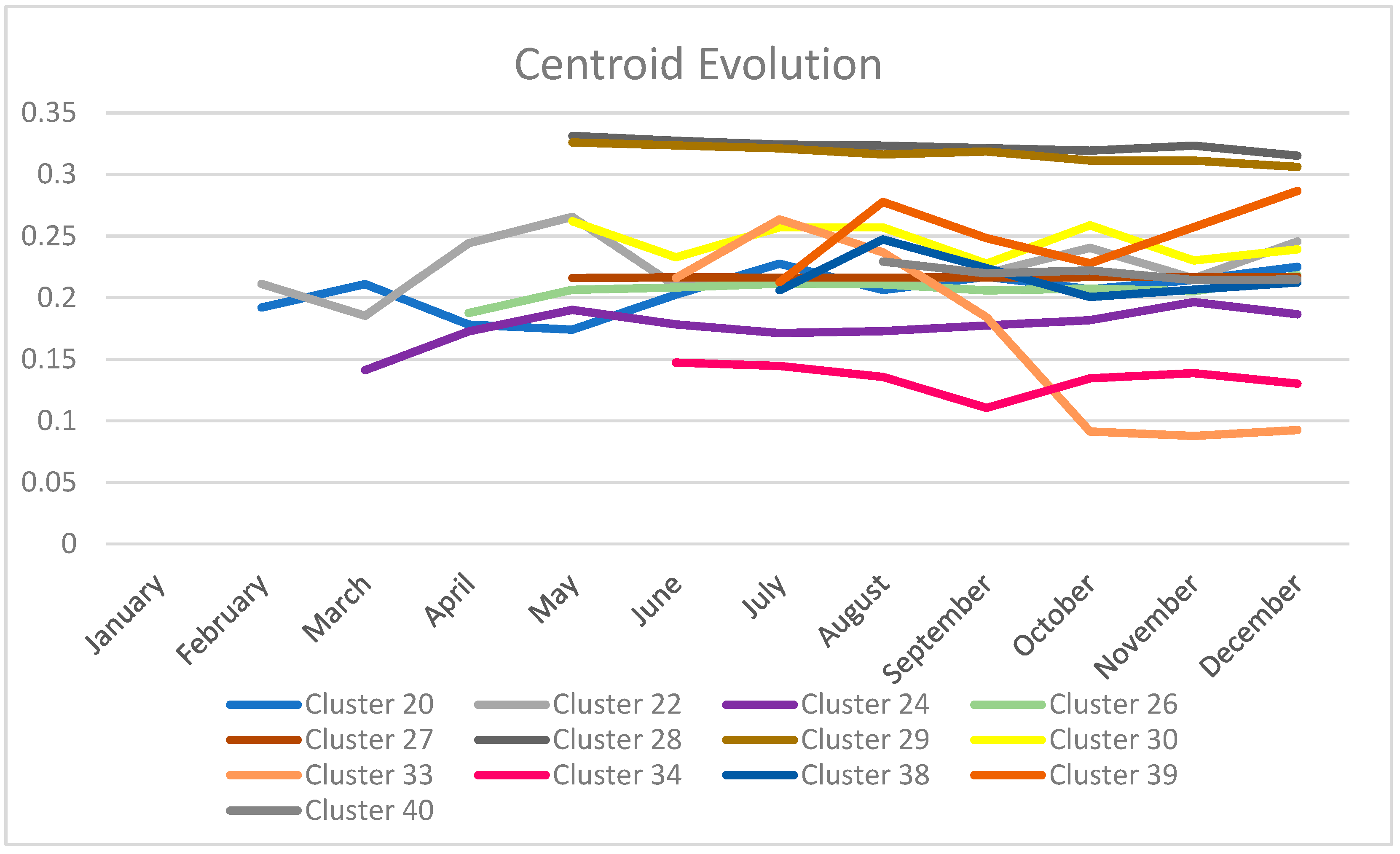
4. Analysis of the Evolution of Clusters

In this section, we analyse the evolution of LAMDA clusters by month and quarterly. Subsection one studies in detail how LAMDA is creating and merging the clusters over time, and Section 2 extends the periods to quarters to evaluate the capacity of LAMDA for larger periods. In addition, at the end, we discussed the size of the clusters.

4.1. Initial Experiment

Comparing the evolution of both algorithms, at the end of the execution, there are 20 and 26 clusters for X-means and LAMDA, respectively. In this section, we will analyze the evolution of LAMDA clusters since it presents the best results and has a more dynamic behavior, creating and merging clusters throughout the execution.
We will start by analyzing the creation and merger of clusters shown in Table 2. Table 2 describes the clusters defined each month by LAMDA, indicating which have been merged, generated, etc. Let us remember that the online clustering process is cumulative; that is, the behavior of the previous month is taken into account. Thus Table 2 shows the reference month, the identifier of the clusters formed, the total number of clusters formed at the moment, and also comments where it is mentioned if there is a merger of some clusters, as well as the number of clusters that are added in the month.
Initially, 16 clusters are formed, of which the clusters identified with the numbers 10, 11, and 13 merge with other clusters, leaving a total of 13 in the first month. For the second month, it is observed that, apart from the 13 clusters created the previous month, 6 new clusters are added initially, of which the clusters with id 8, 17, 19, and 21 are merged, leaving a total of 15 clusters. The value of the centroids of clusters 10, 11, and 13 differ only in the variables of light, air coolers, and elevators. Similarly, the value of the centroids of clusters 8, 17, 19, and 21 differ only in the variables of air treatment units and air coolers.
Continuing with the analysis, the first 9 clusters generated in January are maintained throughout the study period. This behavior of creating and merging clusters is maintained until September, generating up to 40 clusters, of which 26 remain. As of September, no new clusters are created nor are there new mergers, such that all new observations/individuals are added to one of the 26 clusters formed so far.

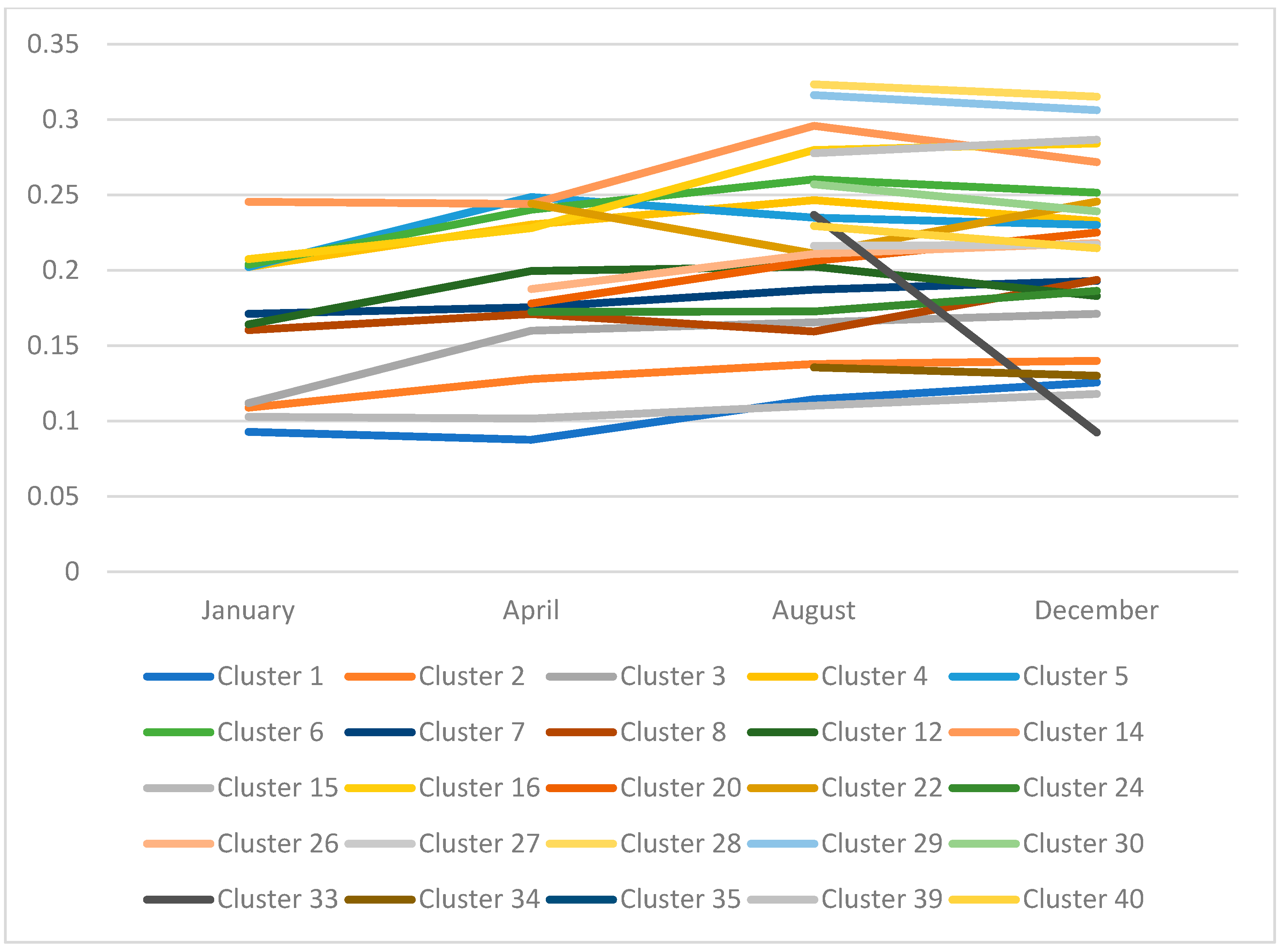
4.2. Quarterly Evolution Analysis

We decide to analyze the evolution of the clusters by quarter. We can see in Figure 6 how the general tendency is to remain stable and follow a predictable trend. The especially erratic behavior that appeared in clusters 19 and 20 in Figure 2 is no longer visible. These clusters have few individuals compared to the rest of the groups, which makes them more volatile to small changes or new inclusions in the cluster. These are clusters that represent patterns with high consumption (more than 700 kW). Cluster 39 has a behavior pattern similar to that of 16, so, over time, if they maintain this trend, it is possible that they will unify because the difference is due to the values of the light and elevators. In the same way, we can study the behavior of 3 clusters that are approaching in December; these are clusters 26, 27, and 40, which are grouped below the 0.22 value. However, this case is different from the previous one since they only approach the end of the analysis, as we can see in Figure 6 (the difference is due to the values of air treatment units and air coolers). In this case, we should be aware of their evolution since the 3 come with different trajectories.
Finally, Figure 7 shows the number of average individuals per cluster through the evolution of the clusters for this period of time. The most populated clusters are 15, 33, and 34. Groups 15 and 34 are quite populated throughout their existence, and 33 goes from being a cluster with few individuals to one with a lot of weight. This change occurs when, in the range of 0.24 in August, it falls to 0.09, where it stabilizes. In these clusters, it can be seen that their trajectory (once they have a high number of elements) is more stable, and only small corrections are made to their centroids as individuals are added to the groups. We see then that the majority of individuals are in these 3 groups. Particularly, in December, its centroids are 15 = 0.170, 33 = 0.092, and 34 = 0.119 (see Figure 6). Cluster 15 represents a pattern with medium consumption (more than 500 kW) due to mainly heat and circulation pumps and heating and hot water. Similarly, cluster 34 represents a pattern with medium consumption (less than 400 kW) due to mainly cooling, air coolers, and air treatment units. Finally, cluster 33 is a pattern of low consumption (less than 300 kW).
In Figure 7, we see how most of the elements/individuals have been assigned in these 3 clusters. Between them, they occupy almost 90% of the data occupation; the rest of the data is found in the remaining 23 clusters. With this, we can see that most of the elements are in the medium and low threshold of consumption; the centroid with the highest value of this trio of clusters is that of cluster 15 with 0.17 (less than 600 kW).
Let us analyze cluster 33, which has more individuals. This cluster’s trend (evolution) reflects a fall in the last quarter of the year, which may be due to the fact that the use of these office/laboratory spaces is reduced at that time of the year. We can see the next values in the centroid variables, the average consumption of light of 3.5 kW, the average consumption of the heat pump of 24.2 kW, the average consumption of air treatment units of 2.8 kW, and the average consumption of circulation pumps of 0.42 kW. They reflect a space with a moderate consumption of energy, mainly derived from the consumption of the heat pump. As this is the device with the highest consumption, its use in heating and cooling tasks could be analyzed to optimize it.
As can be seen, the detailed analysis, both at the temporal level and at the level of the values of a pattern, allows two things: i) the determination of the energy behavior over time to establish temporary improvement measures (for example, in the months of greatest consumption search for less expensive energy sources) and ii) the determination of the devices that consume the most and the reason they do, in order to establish strategies that optimize them.

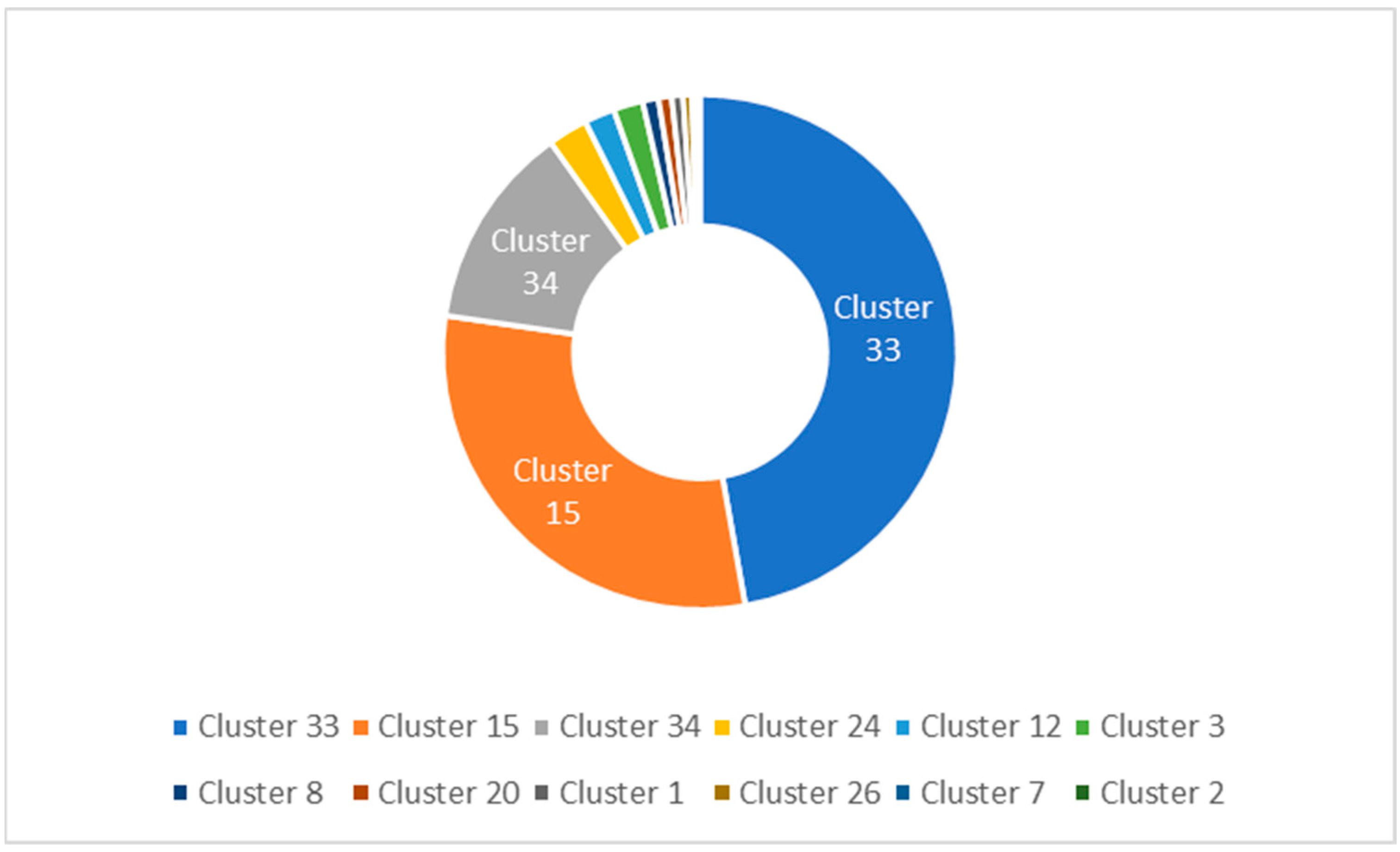
5. Comparison in Different Datasets

To show the feasibility of the energy consumption evolution analysis process based on our online clustering algorithms, several energy consumption datasets are used in this section. Table 3 shows in the first column where the datasets were drawn from and, in the following columns, the quality of the techniques in each of the performance measures analyzed in the work. Thus, Table 3 describes the performance metrics of each technique on different datasets. This allows us to determine if the clusters obtained in each case are of high quality.
According to the results, we see that LAMDA is a very robust method. In particular, in the different datasets, it obtains the best result. It is a very robust algorithm regardless of the energy consumption dataset (time series type). In addition, we see in the previous results (see Section 5) the ability of LAMDA to create or merge clusters over time to adapt to the context.

6. Conclusions

In this work, we have performed online clustering algorithms to analyze the evolutionary behavior of energy consumption patterns, understood as the centroids of the groups they propose. By using X-means and LAMDA, we are able to delegate decision-making about the number of clusters to the algorithms. This was particularly shown in LAMDA since it was able to increase and/or decrease the number of groups. In X-Means, we could not see this behavior since it created the maximum number of clusters from the first iteration. On the other hand, an analysis without a cluster limit is more appropriate in a real scenario (for example, in the case of X-means, the values of K were bounded in one case), regardless of the time it takes. In addition, with X-Means the abnormal behavior of some clusters was observed (affected by outliers).
The analysis of the centroids with LAMDA has made clear the great difference in consumption between users. In addition, according to its evolution, the consumption trends can be studied. In short, the analysis of the evolution of the centroids of the groups allows us to make more precise decisions in the energy world (months of higher consumption, abnormal behavior, etc.). Thus, something relevant is how the variables that generate more energy consumption can be analyzed, particularly the evolution of this consumption through the months (for example, cluster 33 in Figure 6). In general, in the patterns that represent high energy consumption, the variables responsible for this high energy consumption are clearly identified. Normally, these variables, in some cases were heat and circulation pumps and heating and hot water, and in others, the variables were air treatment units, cooling, and air coolers. These combinations of variables are closely linked to high consumption. Likewise, there is a relationship between these variables with respect to the time of year, due to the environmental impact of the time of year on these variables. On the other hand, it can also be identified in the centroids that the variables that have very little impact on energy consumption are light and elevators.
Thus, we have shown in this work the feasibility of using online unsupervised learning approaches to monitor energy consumption patterns. In addition, with our approach, it is possible to analyze and explain in detail the evolution of energy consumption using the cluster centroids, with which it is possible to study their behavior over time and determine the specific energy behavior of the devices. With both, optimization strategies can be defined, both at a global level (according to the customer’s consumption trend) and at a specific level (in the devices).
In general, the pattern of energy consumption behavior of a customer/user can be used by both suppliers and consumers. In the case of consumers, know their energy consumption and, based on this, optimize it and carry out the optimal management of it, among other things, in the case of suppliers trying to adapt their offer to the needs of users, among other things. One of the limitations of this work is that it has been carried out with datasets, but in a real context, a robust platform will be required that captures the different energy consumption values of the different devices to be monitored in real time. Another limitation is the dependence on the quality of the data from the clustering process, which may affect the quality of the results when there are many atypical values, missing data, among other aspects.
Some aspects to take into account for future work are: (i) having data on energy consumption (applied in our case) together with a user profile to favor a more complete and specific analysis (for example, profiling the energy behavior of an individual) and (ii) having an automatic construction of the analysis of the evolution of the clusters would be ideal (give more explainability to the centroids that are obtained) to help decision-makers. Therefore, a future work should define hybrid models that combine online clustering algorithms with techniques that allow predicting some of the energy variables. In addition, this work will be extended to analyze these patterns using explainability techniques to establish an interpretability of the patterns from the behavior of the attributes that make up the centroids. Finally, future works will use these results in an intelligent energy management system in order to personalize their behavior in the function of the consumer’s energy pattern.

Author Contributions

Conceptualization, J.A.; Methodology, J.A., M.R.-M. and C.Q.-G.; Software, J.V. and C.Q.-G.; Validation, J.V.; Formal analysis, J.A.; Investigation, J.A.; Resources, M.R.-M.; Writing—original draft, J.A.; Writing—review & editing, M.R.-M. All authors have read and agreed to the published version of the manuscript.

Funding

J.A. is supported by the European Union’s Horizon 2020 research and innovation programme under the Marie Skłodowska-Curie grant agreement No 754382 GOT ENERGY TALENT. M.D. R-Moreno is supported by the JCLM project SBPLY/19/180501/000024 and the Spanish Ministry of Science and Innovation project PID2019-109891RB-I00, both under the European Regional Development Fund (FEDER).

Data Availability Statement

The data sets used in this work have been retrieved from the article repositories [31,34,35,36,37,38,39].

Conflicts of Interest

The authors declare no conflict of interest.

Disclaimer

The content of this publication does not reflect the official opinion of the European Union. Responsibility for the information and views expressed herein lies entirely with the author(s).

References

  1. Akkaya, K.; Guvenc, I.; Aygun, R.; Pala, N.; Kadri, A. IoT-based occupancy monitoring techniques for energy-efficient smart buildings. In Proceedings of the IEEE Wireless Communications and Networking Conference Workshops (WCNCW), New Orleans, LA, USA, 9–12 March 2015. [Google Scholar] [CrossRef]
  2. Patel, K.; Patel, S. Internet of Things-IOT: Definition, Characteristics, Architecture, Enabling Technologies, Application & Future Challenges. Int. J. Eng. Sci. Comput. 2016, 6, 6122–6131. [Google Scholar]
  3. Gray, C.; Ayre, R.; Hinton, K.; Campbell, L. ‘Smart’ Is Not Free: Energy Consumption of Consumer Home Automation Systems. IEEE Trans. Consum. Electron. 2020, 66, 87–95. [Google Scholar] [CrossRef]
  4. Yang, R.; Wang, L. Development of multi-agent system for building energy and comfort management based on occupant behaviors. Energy Build. 2013, 56, 1–7. [Google Scholar] [CrossRef]
  5. Fotopoulou, E.; Zafeiropoulos, A.; Terroso-Sáenz, F.; Şimşek, U.; González-Vidal, A.; Tsiolis, G.; Gouvas, P.; Liapis, P.; Fensel, A.; Skarmeta, A. Providing Personalized Energy Management and Awareness Services for Energy Efficiency in Smart Buildings. Sensors 2017, 17, 2054. [Google Scholar] [CrossRef]
  6. Aguilar, J.; Garces-Jimenez, A.; R-Moreno, M.; García, R. A systematic literature review on the use of artificial intelligence in energy self-management in smart buildings. Renew. Sustain. Energy Rev. 2021, 151, 111530. [Google Scholar] [CrossRef]
  7. Escobar, L.M.; Aguilar, J.; Garcés-Jiménez, A.; De Mesa, J.A.G.; Gomez-Pulido, J.M. Advanced Fuzzy-Logic-Based Context-Driven Control for HVAC Management Systems in Buildings. IEEE Access 2020, 8, 16111–16126. [Google Scholar] [CrossRef]
  8. Yoon, G.; Park, S.; Park, S.; Lee, T.; Kim, S.; Jang, H.; Lee, S.; Park, S. Prediction of machine learning base for efficient use of energy infrastructure in smart city. In Proceedings of the International Conference on Computing, Electronics & Communications Engineering (iCCECE), London, UK, 22–23 August 2019; pp. 32–35. [Google Scholar]
  9. Wu, Z.; Chu, W. Sampling strategy analysis of machine learning models for energy consumption prediction. In Proceedings of the IEEE 9th International Conference on Smart Energy Grid Engineering, Oshawa, ON, Canada, 11–13 August 2021; pp. 77–81. [Google Scholar] [CrossRef]
  10. Xiao, Q.; Li, C.; Tang, Y.; Chen, X. Energy Efficiency Modeling for Configuration-Dependent Machining via Machine Learning: A Comparative Study. Tase 2021, 18, 717–730. [Google Scholar] [CrossRef]
  11. Zhang, N.; Shetty, D. An effective LS-SVM-based approach for surface roughness prediction in machined surfaces. Neurocomputing 2016, 198, 35–39. [Google Scholar] [CrossRef]
  12. Abdulshahed, A.M.; Longstaff, A.; Fletcher, S.; Potdar, A. Thermal error modelling of a gantry-type 5-axis machine tool using a Grey Neural Network Model. J. Manuf. Syst. 2016, 41, 130–142. [Google Scholar] [CrossRef] [Green Version]
  13. Kong, D.; Chen, Y.; Li, N. Gaussian process regression for tool wear prediction. Mech. Syst. Signal Process. 2018, 104, 556–574. [Google Scholar] [CrossRef]
  14. Bashawyah, D.A.; Qaisar, S.M. Machine learning based short-term load forecasting for smart meter energy consumption data in london households. In Proceedings of the IEEE 12th International Conference on Electronics and Information Technologies, Lviv, Ukraine, 19–21 May 2021; pp. 99–102. [Google Scholar] [CrossRef]
  15. Olanrewaju, O.A. Predicting industrial sector’s energy consumption: Application of support vector machine. In Proceedings of the IEEE International Conference on Industrial Engineering and Engineering Management, Macao, China, 15–18 December 2019; pp. 1597–1600. [Google Scholar] [CrossRef]
  16. Chu, W.; Spinella, L.; Shirley, D.; Ho, P. Effects of wiring density and pillar structure on chip package interaction for advanced cu low-k chips. In Proceedings of the IEEE International Reliability Physics Symposium, Dallas, TX, USA, 28 April–30 May 2020. [Google Scholar] [CrossRef]
  17. Darlis, D.N.; Latip, M.A.; Zaini, N.; Norhazman, H. Random forest approach for energy consumption behavior analysis. In Proceedings of the IEEE Symposium on Industrial Electronics & Applications, Kuala Lumpur, Malaysia, 17–18 July 2020. [Google Scholar] [CrossRef]
  18. Aguilar, J.; Cerrada, M.; Hidrobo, F. A Methodology to Specify Multiagent Systems; Lecture Notes in Computer Science 4496; Springer: Berlin/Heidelberg, Germany, 2007; pp. 92–101. [Google Scholar] [CrossRef]
  19. Aguilar, J.; Salazar, C.; Velasco, H.; Monsalve-Pulido, J.; Montoya, E. Comparison and Evaluation of Different Methods for the Feature Extraction from Educational Contents. Computation 2020, 8, 30. [Google Scholar] [CrossRef]
  20. Aguilar, J. Definition of an energy function for the random neural to solve optimization problems. Neural Netw. 1998, 11, 731–737. [Google Scholar] [CrossRef]
  21. Müller, A.C.; Guido, S. Introduction to Machine Learning with Python, 1st ed.; O’Reilly Media, Inc.: Sebastopol, CA, USA, 2016. [Google Scholar]
  22. Bagirov, A.M.; Karmitsa, N.; Taheri, S. Partitional Clustering via Nonsmooth Optimization, 1st ed.; Springer: Berlin/Heidelberg, Germany, 2020. [Google Scholar]
  23. Camargo, E.; Aguilar, J.; Quintero, Y.; Rivas, F.; Ardila, D. An incremental learning approach to prediction models of SEIRD variables in the context of the COVID-19 pandemic. Health Technol. 2022, 12, 867–877. [Google Scholar] [CrossRef] [PubMed]
  24. Pelleg, D.; Moore, A. X-means: Extending K-means with Efficient Estimation of the Number of Clusters. Mach. Learn. 2002, 1, 727–734. [Google Scholar]
  25. Pham, D.; Dimov, S.; Nguyen, C. Selection of K in K -means clustering. Inst. Mech. Eng. Part C-J. Mech. Eng. Sci. 2005, 219, 103–119. [Google Scholar] [CrossRef] [Green Version]
  26. Morales, L.; Aguilar, J. An Automatic Merge Technique to Improve the Clustering Quality Performed by LAMDA. IEEE Access 2020, 8, 162917–162944. [Google Scholar] [CrossRef]
  27. Morales, L.; Ouedraogo, C.; Aguilar; Chassot, C.; Medjiah, S.; Drira, K. Experimental comparison of the diagnostic capabilities of classification and clustering algorithms for the QoS management in an autonomic IoT platform. Serv. Oriented Comput. Appl. 2019, 13, 199–219. [Google Scholar] [CrossRef]
  28. Mizumoto, M. Pictorial representations of fuzzy connectives, Part I: Cases of t-norms, t-conorms and averaging operators. Fuzzy Sets Syst. 1989, 31, 217–242. [Google Scholar] [CrossRef]
  29. Ruiz, F.A.; Isaza, C.V.; Agudelo, A.F.; Agudelo, J.R. A new criterion to validate and improve the classification process of LAMDA algorithm applied to diesel engines. Eng. Appl. Artif. Intell. 2017, 60, 117–127. [Google Scholar] [CrossRef]
  30. Bedoya, C.; Uribe, C.; Isaza, C. Unsupervised feature selection based on fuzzy clustering for fault detection of the Tennessee Eastman process. In Advances in Artificial Intelligence; Springer: Berlin/Heidelberg, Germany, 2012; pp. 350–360. [Google Scholar]
  31. Royapoor, M.; Pazhoohesh, M.; Davison, P.; Patsios, C.; Walker, S. Building as a virtual power plant, magnitude and persistence of deferrable loads and human comfort implications. Energy Build. 2020, 213, 109794. [Google Scholar] [CrossRef]
  32. Rousseeuw, P.J. Silhouettes: A graphical aid to the interpretation and validation of cluster analysis. J. Comput. Appl. Math. 1987, 20, 53–65. [Google Scholar] [CrossRef]
  33. Davies, D.L.; Bouldin, D.W. A Cluster Separation Measure. IEEE Trans. Pattern Anal. Mach. Intell. 1979, 1, 224–227. [Google Scholar] [CrossRef] [PubMed]
  34. Papaioannou, T.; Stamoulis, G. Teaming and competition for demand-side management in office buildings. In Proceedings of the IEEE International Conference on Smart Grid Communications (SmartGridComm), Dresden, Germany, 23–27 October 2017; pp. 332–337. [Google Scholar]
  35. Power Consumption Data of a Hotel Building. Available online: https://ieee-dataport.org/documents/power-consumption-data-hotel-building (accessed on 1 July 2022).
  36. Zhang, L.; Wen, J. Data for: A Systematic Feature Selection Procedure for Short-Term Data-Driven Building Energy Forecasting Model Development. Mendeley Data. Available online: https://data.mendeley.com/datasets/r532stprhv/1 (accessed on 1 July 2022).
  37. Zhang, L.; Wen, J. A systematic feature selection procedure for short-term data-driven building energy forecasting model development. Energy Build. 2019, 183, 428–442. [Google Scholar] [CrossRef]
  38. Pipattanasomporn, M.; Chitalia, G.; Songsiri, J.; Aswakul, C.; Pora, W.; Suwankawin, S.; Audomvongseree, K.; Hoonchareon, N. CU-BEMS, smart building electricity consumption and indoor environmental sensor datasets. Sci. Data 2020, 7, 241. [Google Scholar] [CrossRef]
  39. Long-Term Energy Consumption & Outdoor Air Temperature for 11 Commercial Buildings. Available online: https://trynthink.github.io/buildingsdatasets/show.html?title_id=long-term-energy-consumption-outdoor-air-temperature-for-11-commercial-buildings (accessed on 1 July 2022).
Figure 1. Evolution of the centroids of the first 10 groups with X-means.
Energies 16 01649 g001
Figure 2. Evolution of the centroids of the last 10 with X-means.
Energies 16 01649 g002
Figure 3. Bounded clustering with X-Means (Kmax = 15).
Energies 16 01649 g003
Figure 4. Evolution of the centroid of the first groups with LAMDA.
Energies 16 01649 g004
Figure 5. Evolution of the centroid of the last groups with LAMDA.
Energies 16 01649 g005
Figure 6. Evolution of the clusters by quarter with LAMDA.
Energies 16 01649 g006
Figure 7. Partial view of the distribution of elements by cluster.
Energies 16 01649 g007
Table 1. Results of the clustering algorithms.
X-MeansLAMDA
SilhouetteDavies-BouldingSilhouetteDavies-Boulding
January0.4460.6200.6940.305
February0.3880.6450.5210.396
March0.3890.6040.5140.278
April0.3840.6140.5410.238
May0.3460.5890.5630.217
June0.3900.5980.5130.233
July0.3870.6260.5610.321
August0.3820.6140.5910.348
September0.3770.5970.5150.423
October0.3860.6030.5280.248
November0.3840.6380.5190.321
December0.3810.5990.5160.294
Table 2. Creating and merging clusters with LAMDA.
MonthId of Clusters CreatedTotal of ClustersComments
11, 2, 3, 4, 5, 6, 7, 8, 9, 12, 14, 15, 161316 clusters formed and the next clusters are merged: 10, 11 and 13
21, 2, 3, 4, 5, 6, 7, 8, 9, 12, 14, 15, 16, 20, 22156 additional clusters are formed and the next clusters are merged: 17, 18, 19 and 21
31, 2, 3, 4, 5, 6, 7, 8, 9, 12, 14, 15, 16, 20, 22, 24162 additional clusters are formed and the next cluster is generated: 23
41, 2, 3, 4, 5, 6, 7, 8, 9, 12, 14, 15, 16, 20, 22, 24, 26172 additional clusters are formed and the next cluster is generated: 25
51, 2, 3, 4, 5, 6, 7, 8, 9, 12, 14, 15, 16, 20, 22, 24, 26, 27, 28, 29, 30214 additional clusters are formed and there is no fusion
61, 2, 3, 4, 5, 6, 7, 8, 9, 12, 14, 15, 16, 20, 22, 24, 26, 27,28, 29, 30, 33, 3423Form 4 additional clusters and merge 31 and 32
71, 2, 3, 4, 5, 6, 7, 8, 9, 12, 14, 15, 16, 20, 22, 24, 26, 27, 28, 29, 30, 33, 34, 38, 3925Form 5 additional clusters and merge: 35 36 and 37
81, 2, 3, 4, 5, 6, 7, 8, 9, 12, 14, 15, 16, 20, 22, 24, 26, 27, 28, 29, 30, 33, 34, 38, 39, 40261 additional cluster is formed and there is no fusion
91, 2, 3, 4, 5, 6, 7, 8, 9, 12, 14, 15, 16, 20, 22, 24, 26, 27, 28, 29, 30, 33, 34, 38, 39, 4026No additional cluster formation
101, 2, 3, 4, 5, 6, 7, 8, 9, 12, 14, 15, 16, 20, 22, 24, 26, 27, 28, 29, 30, 33, 34, 38, 39, 4026No additional cluster formation
111, 2, 3, 4, 5, 6, 7, 8, 9, 12, 14, 15, 16, 20, 22, 24, 26, 27, 28, 29, 30, 33, 34, 38, 39, 4026No additional cluster formation
121, 2, 3, 4, 5, 6, 7, 8, 9, 12, 14, 15, 16, 20, 22, 24, 26, 27, 28, 29, 30, 33, 34, 38, 39, 4026No additional cluster formation
Table 3. Results of the clustering models in different datasets.
DatasetAlgorithmDavies-BouldingSilhouette
[34]X-Means0.3490.893
LAMDA0.1440.892
[35]X-Means0.3310.575
LAMDA0.2510.660
[36,37]X-Means0.3950.530
LAMDA0.2570.633
[38]X-Means0.6450.635
LAMDA0.2910.690
[39]X-Means0.4150.625
LAMDA0.1770.669
Disclaimer/Publisher’s Note: The statements, opinions and data contained in all publications are solely those of the individual author(s) and contributor(s) and not of MDPI and/or the editor(s). MDPI and/or the editor(s) disclaim responsibility for any injury to people or property resulting from any ideas, methods, instructions or products referred to in the content.

