1. Introduction
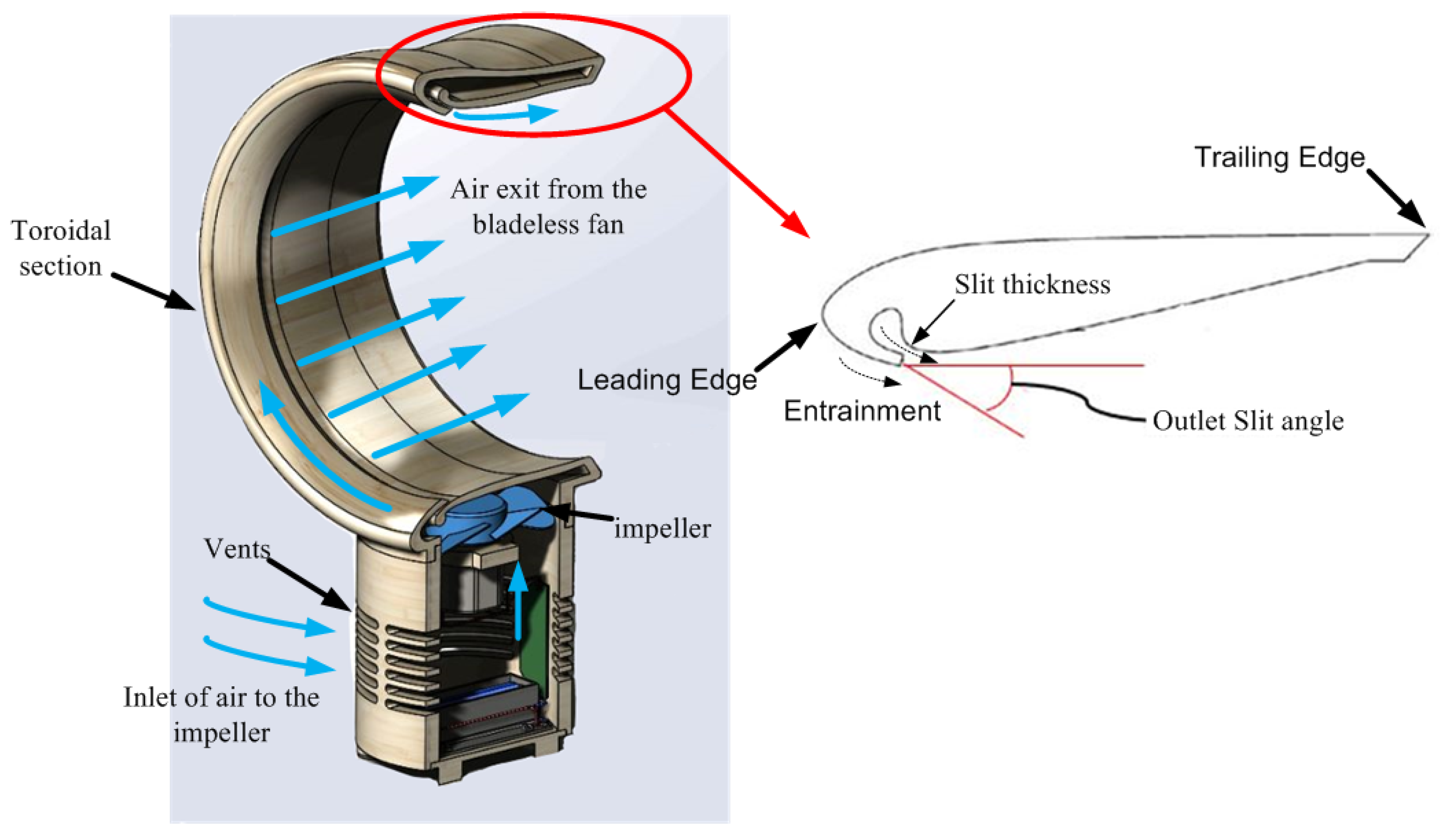
Fans (axial and radial) are used for various applications, such as cooling systems, air conditioning, and ventilation in tunnels and underground spaces. The performance of fans has been enhanced by increasing developments in Computational Fluid Dynamics (CFD) and commercial growth, offering different types of fans with various applications and higher efficacy. The main differences between bladeless and traditional fans are the increasing airflow intake and the lack of a visible impeller. Toshiba devised the bladeless fan (or Air Multiplier) concept in 1981. Researchers such as James Dyson and Jafari et al. further developed it. A bladeless fan is a type of air circulation device that uses no blades or any other moving parts, making the bladeless fan more reliable and energy efficient. From a performance point of view, bladeless fans are better because they multiply mass flow rate, eliminate buffeting, consume less power, and are quieter. However, to function properly, the bladeless fan requires a diffuser on the outlet, which acts as a nozzle to direct the flow of air and create a smooth flow of air out of the outlet. A bladeless fan consists of two main sections: the first is the base that houses the impeller that has vents to suck in air from the surroundings, and passes it through the toroidal section with an airfoil profile, as shown in
Figure 1. Gammack [
1] demonstrated the working of the bladeless fan. Two phenomena responsible for airflow rate multiplication are the Coanda effect and entrainment.
The Coanda effect at the airfoil creates a pressure difference between the two sides of the fan. Air near the leading edge has a lower pressure, while air near the trailing edge has higher pressure. Due to the pressure difference, more air is blown from the leading edge to the trailing edge. Entrainment occurs at the inlet (near the toroidal section) and outlet of the fan. It then passes by the toroidal section, exits from the outlet slit, and multiplies mass flow rates across their ends, improving the outlet velocity. Entrainment sucks in air at the fan’s base and from the back of the fan. The entrainment and multiplication of airflow increase the efficiency of the fan.
Theoretically, discharge ratio is the ratio of the fan’s outlet velocity to the inlet velocity, which is influenced by several factors, such as the outlet slit thickness of the airfoil, the the angle of outlet flow relative to the fan’s axis, the height of the fan cross-section, the aspect ratio of fan’s cross-section and the hydraulic diameter of the fan according to studies conducted by Jafari M. [
2]. The major parameters, such as outlet slit thickness and outlet slit angle, are directly concerned with the flow passage, and thus the author presumes that these parameters have a major influence on the performance of a bladeless fan. In the current work, a preliminary study on a two-dimensional bladeless fan is conducted to understand the flow behaviour when the slit thickness is varied. A three-dimensional analysis assesses the effect of slit thickness and outlet angle.
2. Literature Survey
Very few studies were conducted on Bladeless fans using CFD [
2,
3]. One paper an experimental and numerical analysis of bladeless fans by changing parameters such as the fan cross-section height, flow outlet angle relative to the fan axis, hydraulic diameter, and aspect ratio. CFD analysis identified that the discharge ratio is maximum for a cross-sectional height of 3 cm and an outlet angle of 16
. For aspect ratios greater than 1, the discharge ratio decreases considerably. All profiles used in the present study has an aspect ratio equal to 1. A parabolic velocity profile is ideal for cooling since the maximum velocity is at the centre. The axial fan blast profile, where the velocity is maximum near the edges and reduces at the axis. Jet equations cannot determine the target distance for axial cooling fans. Still, they can be used for bladeless fans since the velocity profile of the output of bladeless fans is parabolic [
2]. The acoustic and aerodynamic performances of fans are the two major advantages of bladeless fans. Bladeless fans are generally quieter than conventional fans owing to their elimination of buffeting. The bladeless fan output is uniform and has the maximum velocity at the centre of its velocity profile, optimal for cooling purposes. Jafari M. [
2] investigated noise levels of a bladeless fan in steady and unsteady flow conditions, using Broadband Noise Source (BNS) and Ffowcs Williams and Hawkings (FW-H) equations [
4] investigated the influence of enlarged impellers, with increments in the impeller diameter and the internal characteristics are studied. The numerical investigation indicated that the outlet slit of air is the primary noise source.
Previous researchers conducted CFD investigations on centrifugal and axial-bladed fans to optimize the mass flow rate and enhance performance. Recently, [
5] performed a behavioral study on maximizing the number of blades on a radial fan. They reported that the mass flow rate at the outlet increases with the number of blades. Furthermore, they performed a transient three-dimensional analysis of standard ceiling fans. Results showed that the ceiling fan could replace the airflow characteristics generated by the fan’s meandering plume and local fine shear layers [
6] performed several simulations to optimize an airfoil profile to enhance mine ventilation fans’ efficiency. Out of six distinct fan profiles, the NACA 747A315 showed the lowest energy consumption and maximum efficiency.
3. Major Parameters Influencing Bladeless Fan
The major parameters influencing the performance of the bladeless fan, such as airfoil profile, outlet thickness, outlet angle and maximum inlet velocity from the impeller, are discussed below.
3.1. Airfoil Profile
The airfoil is the primary working surface for energy transfer, and therefore proper airfoil selection is significant. Eppler 473 has higher curvature offering a good Coanda surface, thus providing better suction of air from the back of the fan. The outlet volume flow rate increased linearly with an increase in the inlet volume flow rate. According to [
7], noise emissions increase with an increased inlet volume flow rate [
8]. Postulated that with increasing curvature of the Coanda surface, several low-pressure regions along the airfoil are gradually enlarged, begin to merge slowly, and finally form a large area of low pressure, thus improving the Coanda effect.
The results of the study by [
9] indicate that the overall performances were substantially equivalent. With a drop of 8% of pressure rise at a conception flow rate for the thick blades fan and maximum efficiency that is 3% lower than the efficiency of the thin blades fan and that is shifted toward lower flow rates. The efficiency of thick airfoils is 3% less than that of thin airfoils with low flow rates. The Eppler’s discharge ratio of 473 airfoils is highest when the thickness of the cross-section is 3 cm [
10]. Declared that thicker blades demand higher power consumption since they add weight to the fan and lead to excess vibration and failure.
3.2. Outlet Slit Thickness
The outlet slit is the gap through which air exits the airfoil profile, as depicted in
Figure 1. The slit thickness is the most influential factor in the discharge ratio. Theoretically, the smaller the slit thickness, the higher the output velocity and the higher the pressure drop, enhancing the Coanda effect [
11] studied the Eppler 473 airfoil profile with a slit thickness of 1 mm and varied slit angle, which produced a maximum discharge ratio for an inlet mass flow rate of 80 LPS.
3.3. Outlet Angle and Velocity
The angle between the horizontal and the normal outlet slit is the outlet angle, as referred to in
Figure 1. The outlet slit angle affects the amount of pressure drop across the airfoil and the convergence distance of the velocity profile.
Figure 1 shows the outlet angle of an airfoil profile. The constraint of the environment binds the outlet velocity. Cooling fans usually have outlet velocities between 2 m/s and 7 m/s. Velocities that are too high will be uncomfortable for occupants.
3.4. Maximum Inlet Velocity
Mohaideen M.M. [
12] analyzed the exit velocity measurements related to inlet velocity and the wake velocity profile. The inlet velocity increased when the blade passage separation decreased. The wake velocity profile showed uniform velocity distribution when the inlet velocity was higher. This concept from fans with blades can be extrapolated to bladeless fans, increasing velocity by reducing slit thickness.
4. CFD Simulation
In the preliminary study, a two-dimensional analysis was carried out to understand the flow pattern and velocity profile at the exit of the bladeless fan. Two-dimensional analysis has shown that the outlet of the bladeless fan is able to provide uniform velocity, and thus, further, the study was extended to a three-dimensional analysis to investigate the influence of outlet slit thickness and angle on the performance of the bladeless fan.
4.1. Geometrical Modeling
Based on Euler’s equations, Raj D. [
13] stated that the energy obtained by the air particles from the fan is directly proportional to the fan’s diameter. The fan’s diameter was 300 mm in the computational setup, and the airfoil chord length was 60 mm. In this study, the outlet slit and outlet angles are varied, and flow behaviour is analyzed. The outlet slit thickness was varied from 1.2 mm to 2 mm with an interval of 0.2 mm. The outlet angles are varied from 16
to 26
with an interval of 2
.
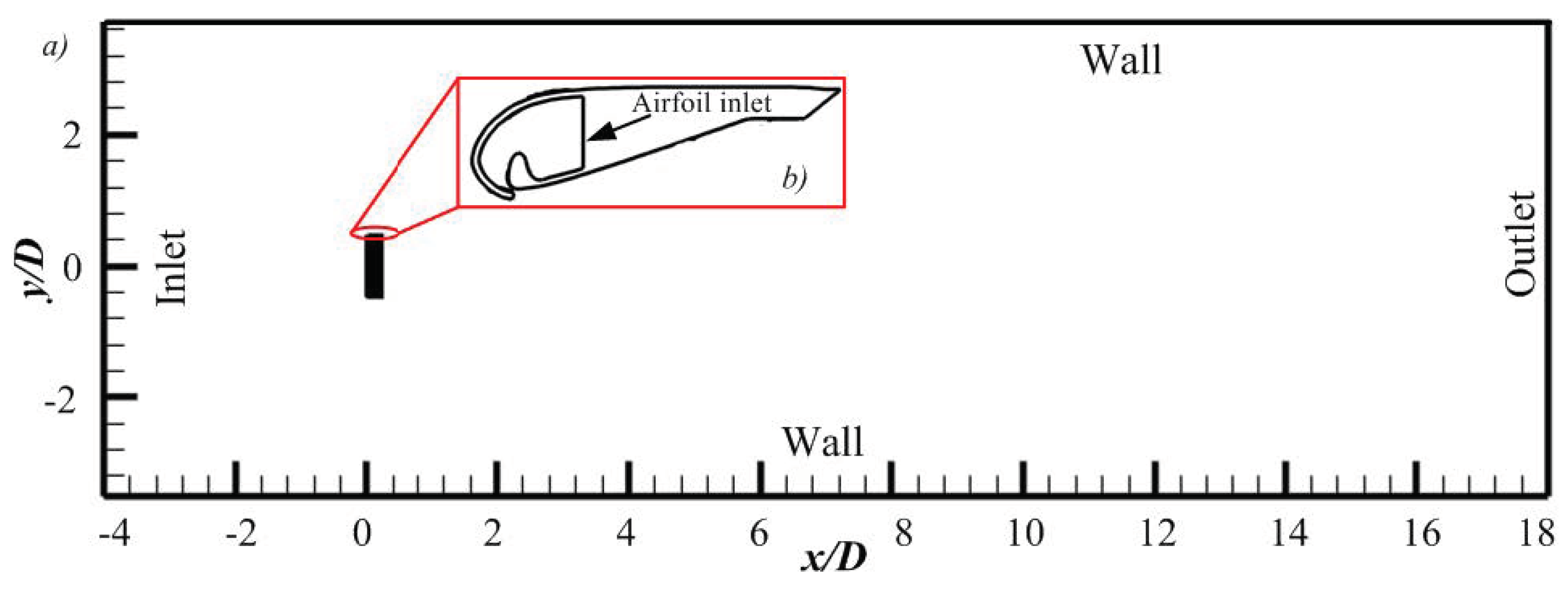
4.2. Computational Domain and Mesh Generation
The computational domain for the two-dimensional analysis is shown in
Figure 2a; the sidewalls of the domain are 2.5D apart and are more than twice the fan diameter. The downstream length is 18D, and the total height is 5D. The boundary conditions are the slow inlet (Inlet) that allows environmental airflow and the inlet through which air from the impeller enters the airfoil (Airfoil inlet). The airfoil profile is set as “walls” and “stationary walls”, representing the room’s ceiling and floor. The bladeless fan is 1 m from the slow inlet.
Figure 2b is a magnified illustration of the inlet within the airfoil.
The first wall distance was calculated using the following equations: Initially, the Reynolds number is calculated to determine whether the flow is laminar or turbulent using Equation (
1).
An empirical coefficient for fully developed turbulent flow is then used to estimate the skin friction coefficient. The skin friction coefficient is calculated using Equation (
2), where
Re is Reynold’s number.
Wall shear stress is calculated using Equation (
3), the free stream the velocity (U), density (
) and skin friction coefficient (
).
Now, the Wall shear stress is calculated as shown in Equation (
4).
Equation (
5)
denotes the distance of the boundary from the centroid of the adjacent cell. The
is calculated using the desired y
value and friction velocity.
Finally, using the value of
, the first layer thickness is given by Equation (
6), where
is the thickness of the first mesh cell from the boundary for inflation layers.
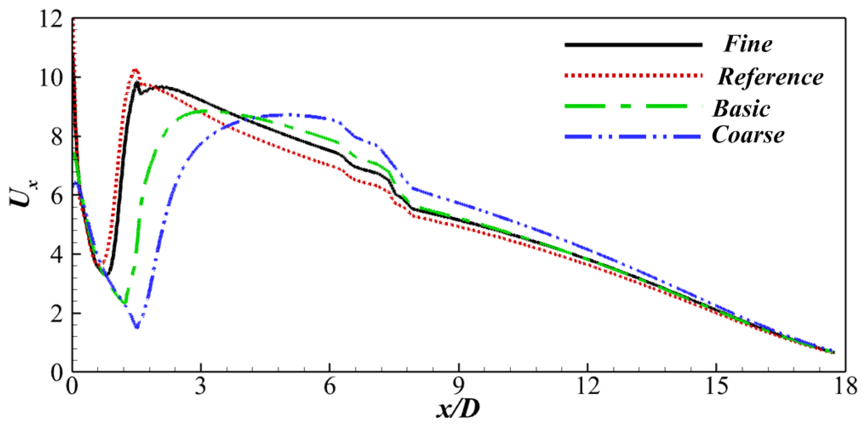
A common problem in numerical simulations is the dependence of results on the grid size. Since grids vary in size due to machine limitations and computational efficiency requirements, it is necessary to determine how the grid size affects the accuracy of the simulation. This is done through the mesh sensitivity test. The sensitivity test was performed on coarse, basic, reference, and fine grids constructed using the above formulas; the details are shown in
Table 1. The downstream velocity is used as a benchmark for grid independence for the sensitivity test.
Figure 3 shows that the fine grid results are close to the reference grid; thus, further simulations are fixed with the fine grid for 3D simulation. For 2D simulations, the poly-hex core mesh was used, and the total mesh count was nearly 7.1 million.
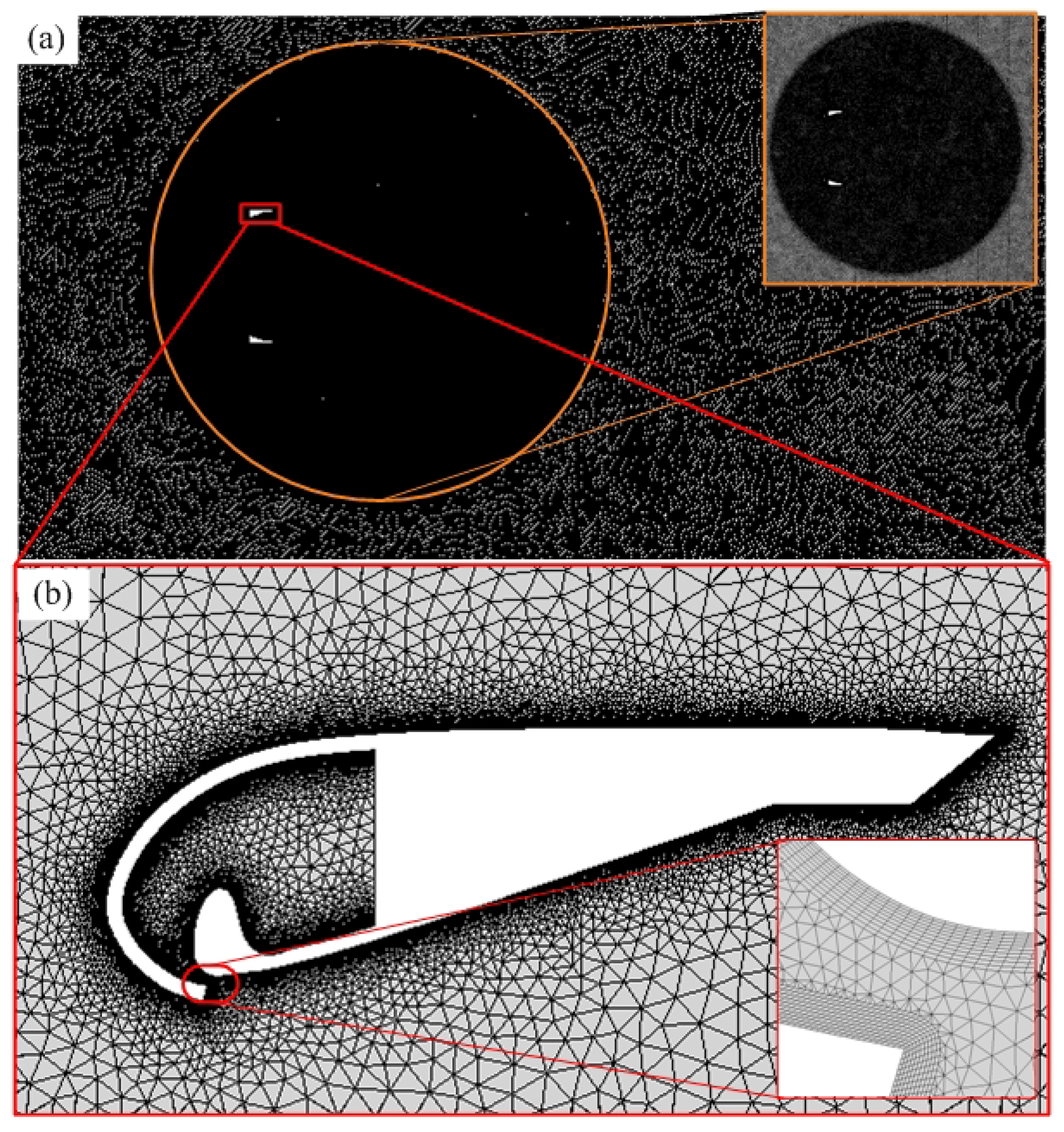
Figure 4a shows the fine mesh around the airfoil as a sphere of influence. The y
value was set to 1 to capture flow features such as pressure, velocity and turbulent kinetic energy near the walls.
Figure 4b is a zoomed-in view of the inflation layer (12 with a growth rate of 1.05) near the outlet slit region of the airfoil. With the use of the above equations, the 3D mesh first wall distance is modelled.
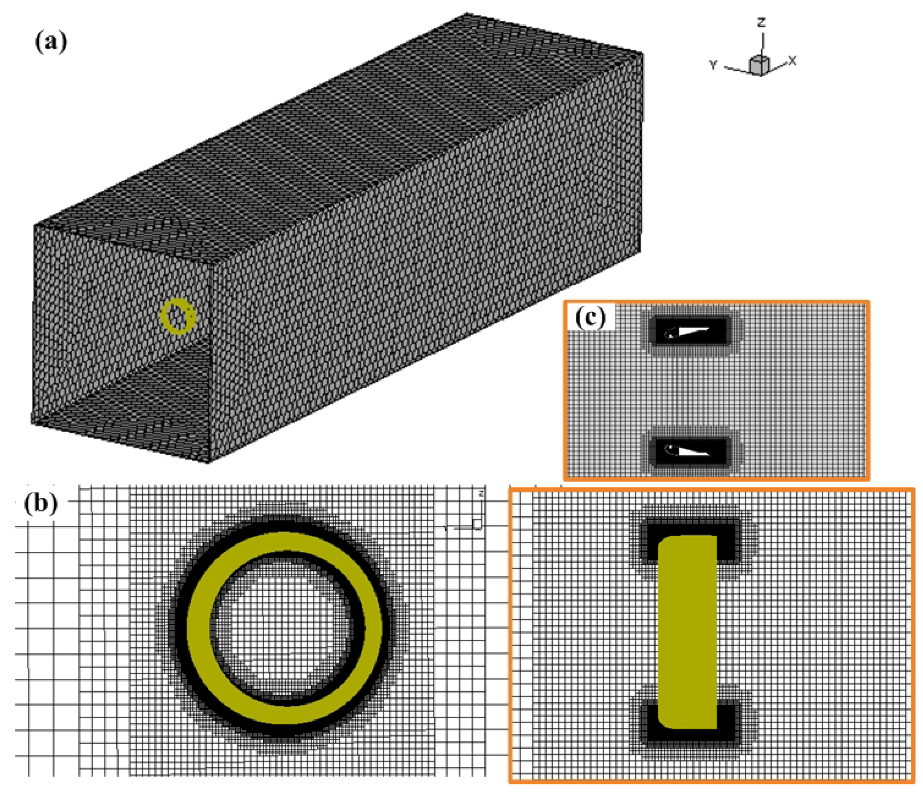
Figure 5a–c shows the detailed view of aerofoil and volume mesh inside the domain. The total number of elements was around 15.4 million cells.
4.3. Turbulence Model and Simulation Set-Up
The 2D and 3D simulations were performed with the commercial CFD code ANSYS Fluent 2021. Both simulations are accomplished using a k-omega SST turbulence model with a pressure-based solver. Both the convection and the viscous terms of the governing equations were discretized at the second order, the pressure interpolation is second order, and the SIMPLE method is utilised for pressure velocity-coupling. Convergence is thought to be accomplished when all the scaled residuals levelled off and reached a minimum of 10 for the continuity, x,y,z velocity, momentum, K, and Omega equations are 10. The k-omega SST turbulence model captures flow features near walls more accurately than other RANS models. A first-layer thickness approach was used to model the inflation layers, which would cover the boundary layers. The equations and formulas required to successfully determine the first layer height based on specific properties such as free stream velocity, density, dynamic viscosity, reference length, and adhered y value are mentioned in detail. In this simulation, the ambient air velocity is kept at 0.005 m/s. The fan inlet velocity varied from 1 m/s to 6 m/s with an interval of 1 m/s. The outlet was set to standard pressure outlet. The solution is initialized using hybrid initialization.
5. Verification and Validation
Results derived from CFD simulation are always affected by various factors. Therefore, it is important to verify that the CFD simulation results are accurate and reliable. The boundary conditions and solver settings must be verified and validated to determine the accuracy and reliability of the simulation [
14]. To validate this simulation’s effectiveness and accuracy, this simulation is validated with previous literature (experiment by Quinn [
5], and CFD by Jafari [
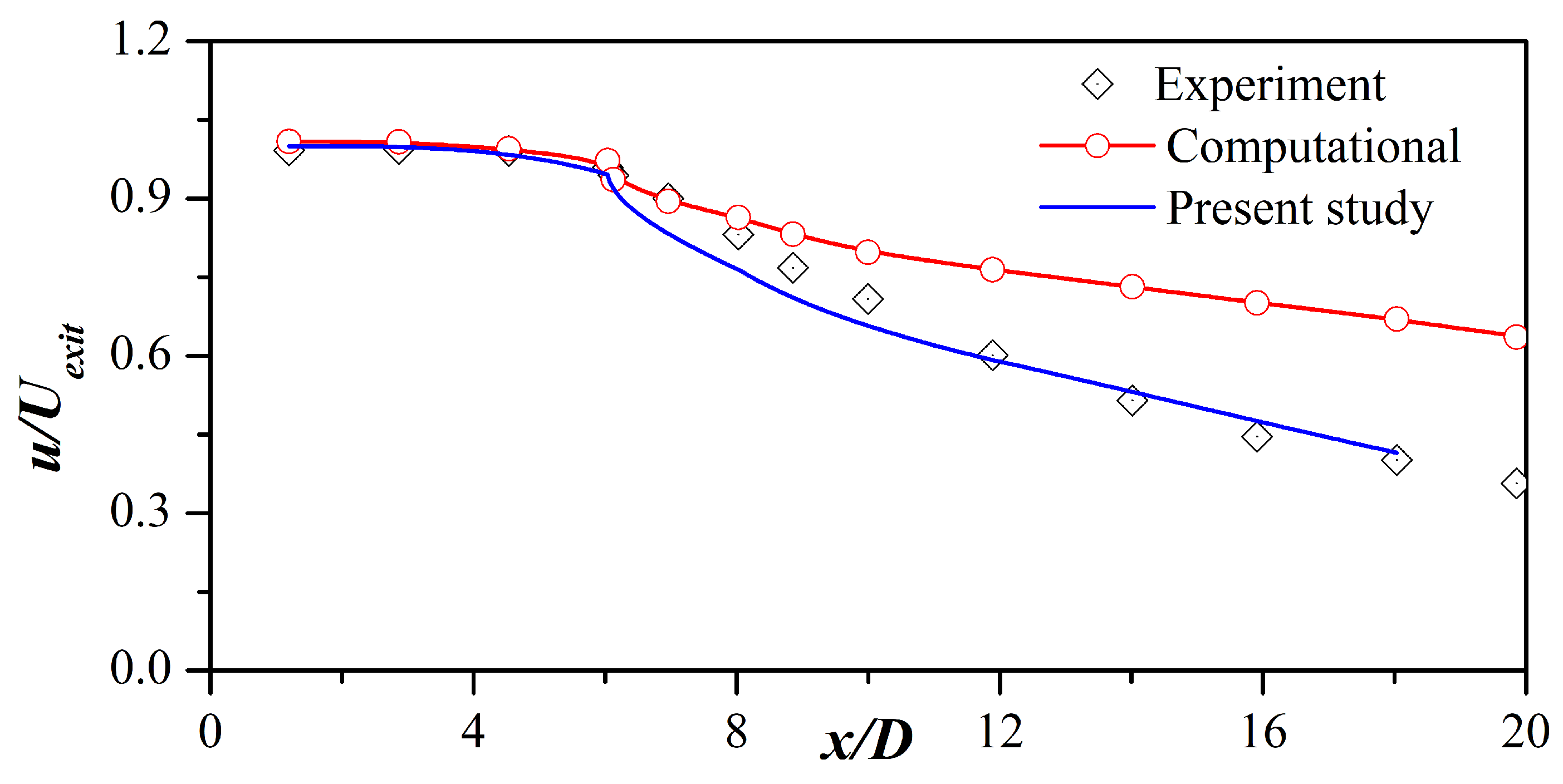
4]). The computed results of the downstream mean velocity are presented in
Figure 6. U is the mean velocity at the centerline, and
is the downstream velocity at the center of the bladeless fan exit (at plane P1, refer to
Figure 7). It was indicated that the downstream velocity profiles shared consistent patterns with previous works. The experimental work of Quinn [
5] results are very close to the present work, which shows the reliability and accuracy of the CFD simulation. In reference to this simulation, the remaining simulations followed the same procedure for different slit angles.
6. Results and Discussion
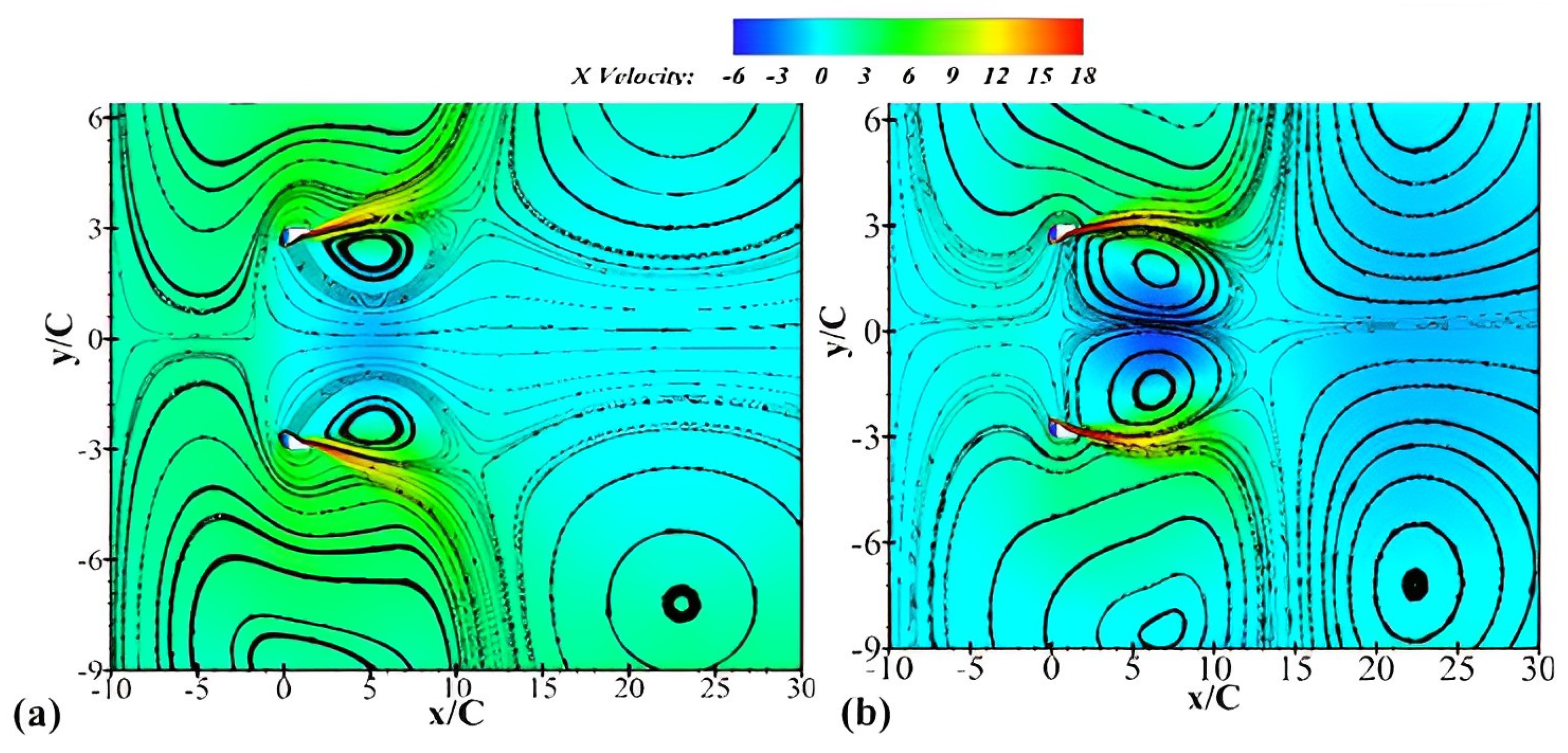
6.1. 2D Flow Analysis of a Bladeless Fan
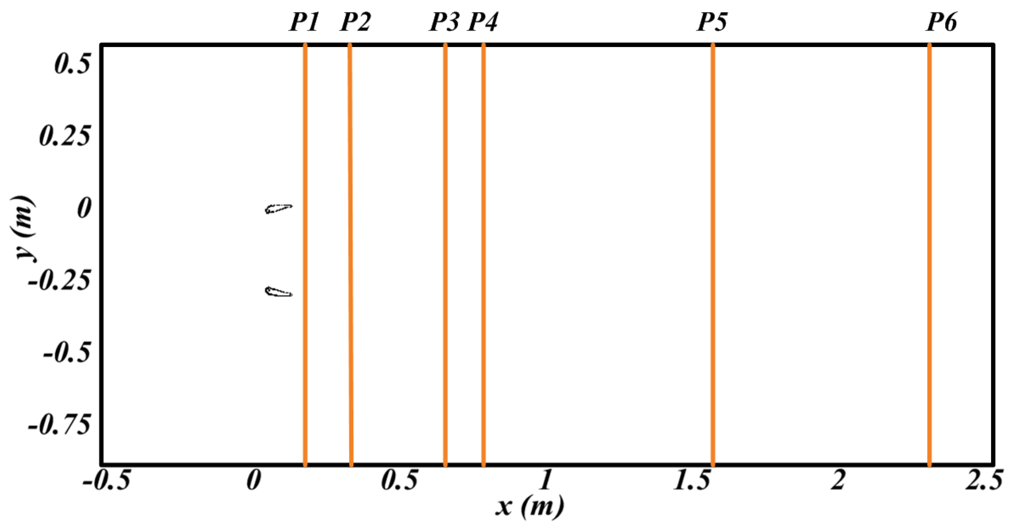
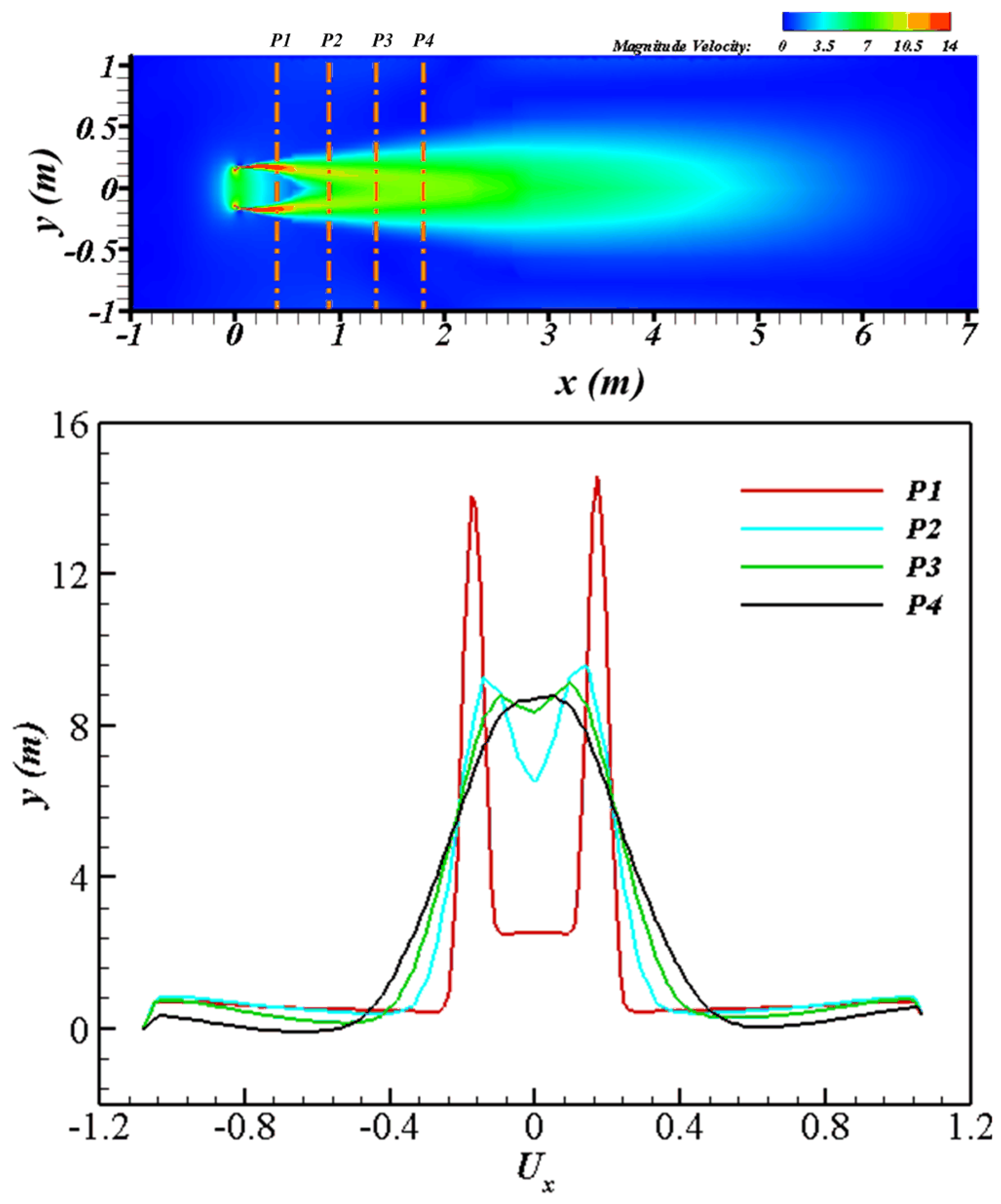
To understand the flow behaviour near the bladeless fan, the results were extracted on various planes (P1, P2, P3, P4, and P5) along with the flow at different distances, as shown in
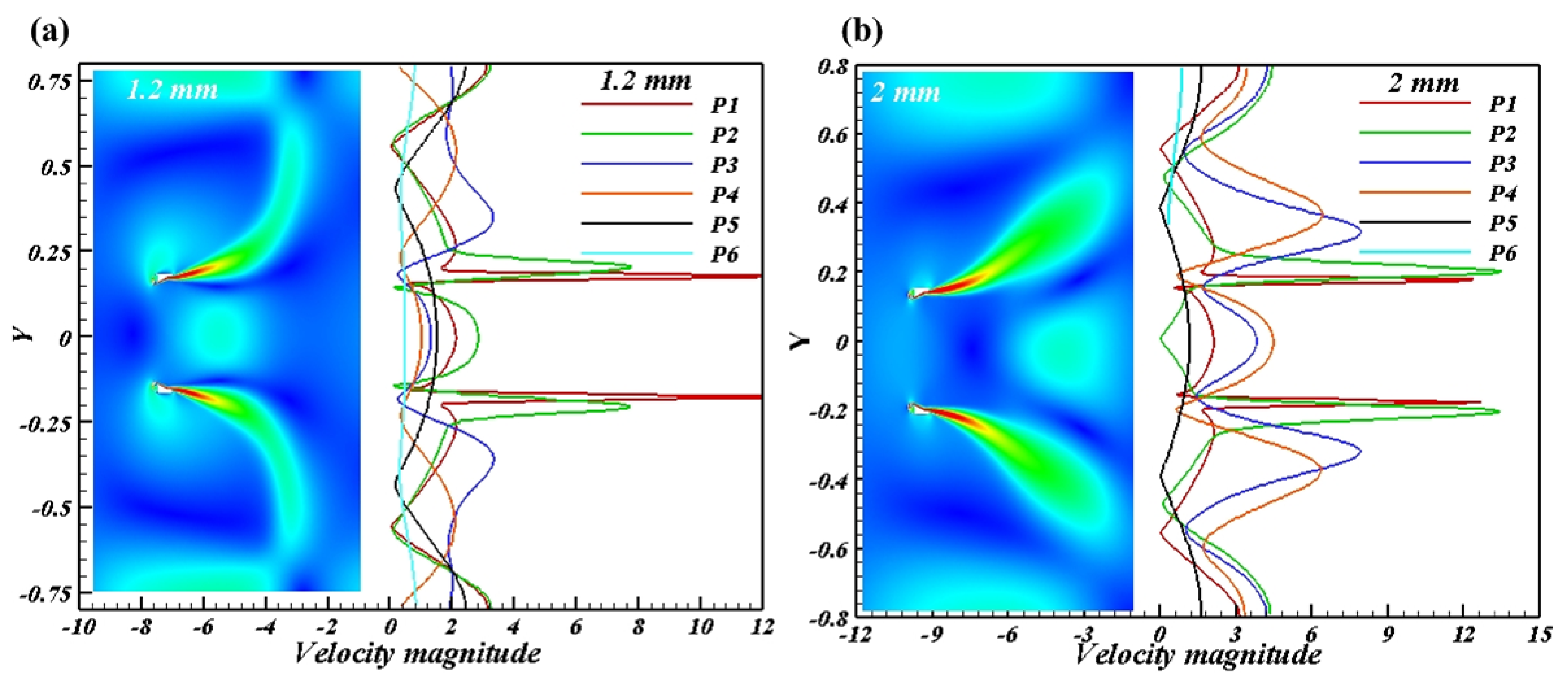
Figure 7. In the defined planes, the flow’s velocity profiles were extracted and plotted in
Figure 8. In
Figure 8, the maximum velocity of 12 m/s at P1 decreases slowly due to circulation. It is clear from
Figure 8a,b that velocity is maximum near the center and decreases with vertical distance. A significant observation is that the velocity profile becomes constant as the distance from the outlet slit increases. P3 values from both slits (
Figure 8) show a substantial peak velocity drop compared with planes 1 and 2. Furthermore, at a distance greater than 0.75 m, the vertical axis velocity profile gradually becomes uniform.
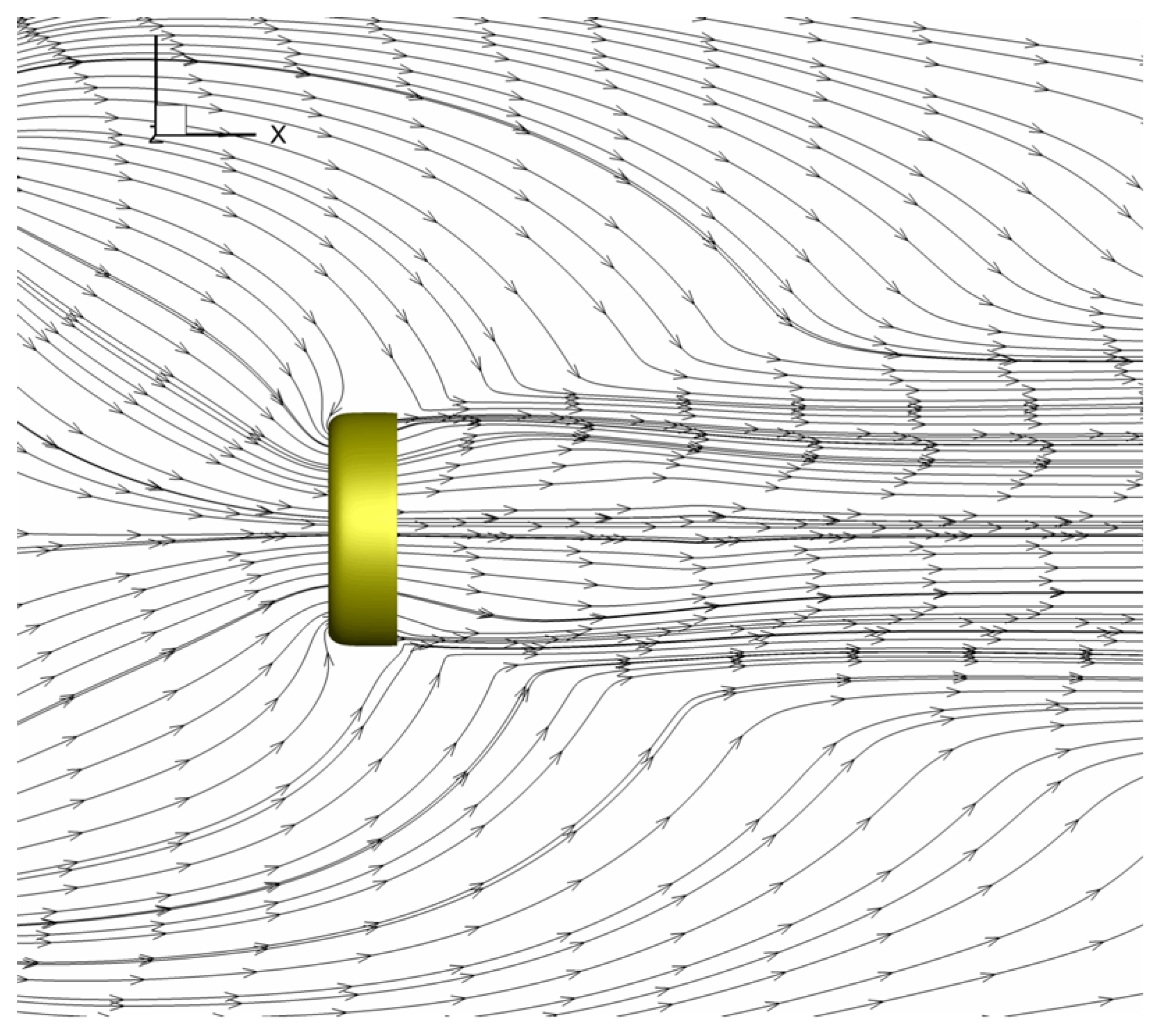
Figure 9a,b represents the streamlined flow in the fan’s immediate environment.
6.2. Flow Analysis of a Bladeless Fan
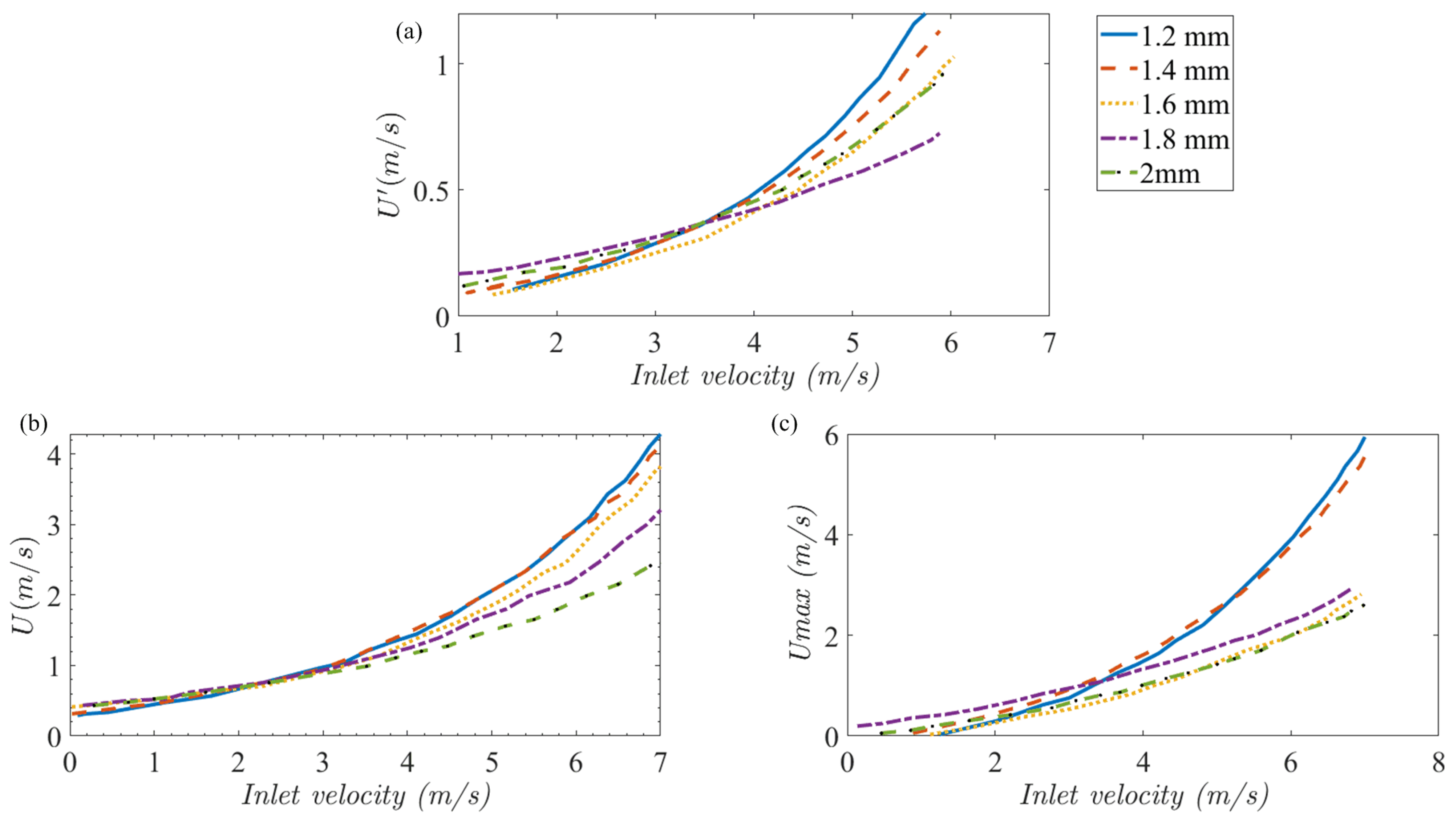
The 3D simulations were carried out similar to the 2D by varying slit thickness from 1.2 mm to 2 mm and with inlet velocities going from 1 m/s through 6 m/s. The main parameters observed in the three-dimensional studies were the velocity profile at 0.9 m from the outlet slit, the standard deviation of outlet velocity, turbulent kinetic energy, symmetry of velocity contours, and optimal distance for occupant location. The graphs presented below compare the above-mentioned parameters from the iterations. In
Figure 10a, the standard deviation of all slits remains almost the same for inlet velocities under 3.3 m/s, and 1.6 mm slit thickness shows the lowest standard deviation up to 5.4 m/s inlet velocity.
Figure 10b plots the average velocity in the occupant area versus the inlet velocity. The outlet velocity is similar for all slits when the inlet velocity is below 2.4 m/s; however, beyond 2.4 m/s, the 1.2 mm slit has the highest average outlet velocity. This velocity also falls in the range for occupant comfort.
Figure 10c shows that optimal maximum velocity is attained for 1.2 mm iteration at lower inlet velocities, reducing input power demand.
The inference from the graphs above is that 1.2 mm slit thickness with 3 m/s inlet velocity yields the best results since its outlet velocity is appropriate for usage and its standard deviation is low. Other iterations have comparable velocities, but their inlet velocity is higher, which demands higher power consumption. The iteration with the lowest slit thickness is more energy efficient to use a change in design rather than increase inlet velocity. The vs. = 1 m/s iteration showed the least standard deviation, while the v = 6 m/s showed the most significant performance. As the inlet velocity increased, the standard deviation of the velocity outlet also increased. The average of the maximum and minimum of the graph is calculated for the final value of standard deviation. The flow moving away from the trailing edge of the bladeless fan has lower turbulence and a more linear airflow profile than other fans. Airflow with low turbulence travels more efficiently from the emission point and loses less energy and velocity to turbulence than conventional fans.
6.3. 3D Flow Features
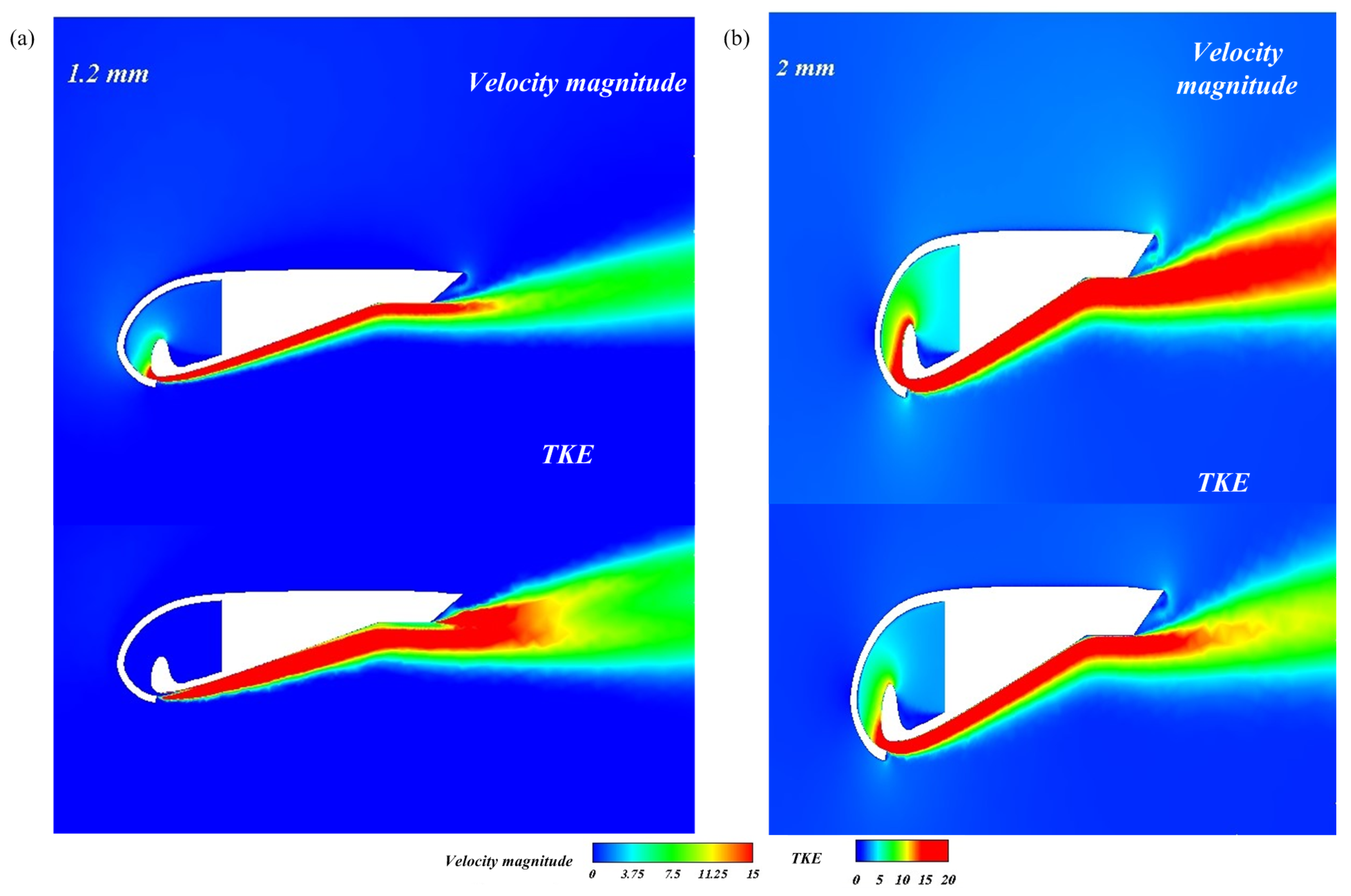
The velocity contour of the 1.2 mm had to be axis-symmetric to be accepted; if the output flow is not symmetric, it will cause discomfort to the occupants.
Figure 11 shows the velocity contour and turbulent kinetic energy of the 1.2 mm slit thickness iteration. The contour is symmetrical about the fan’s horizontal axis.
Figure 11a,b depict bladeless fans’ turbulence kinetic energy and velocity magnitude flow with 1.2 mm and 2 mm slit thicknesses, respectively.
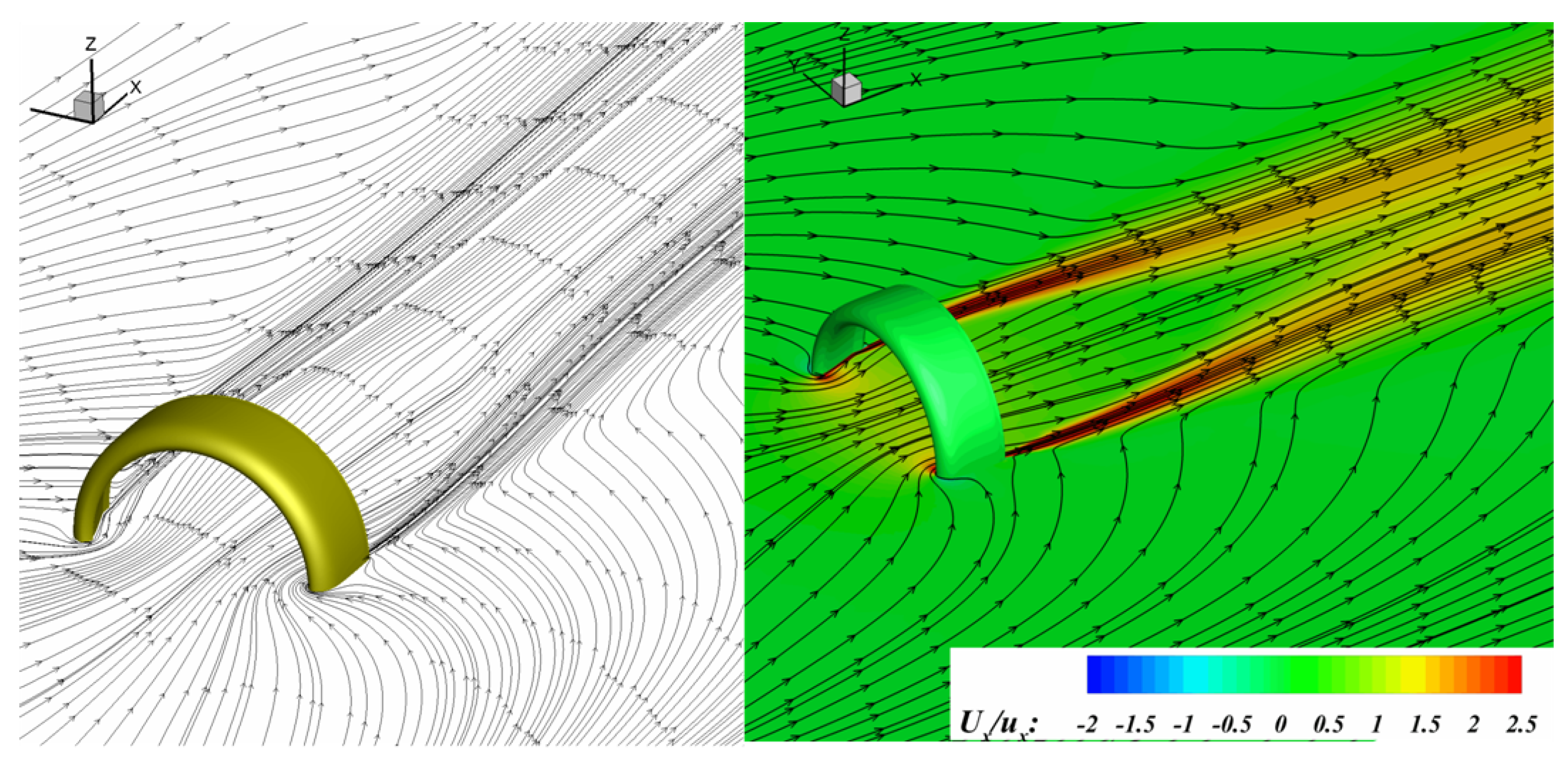
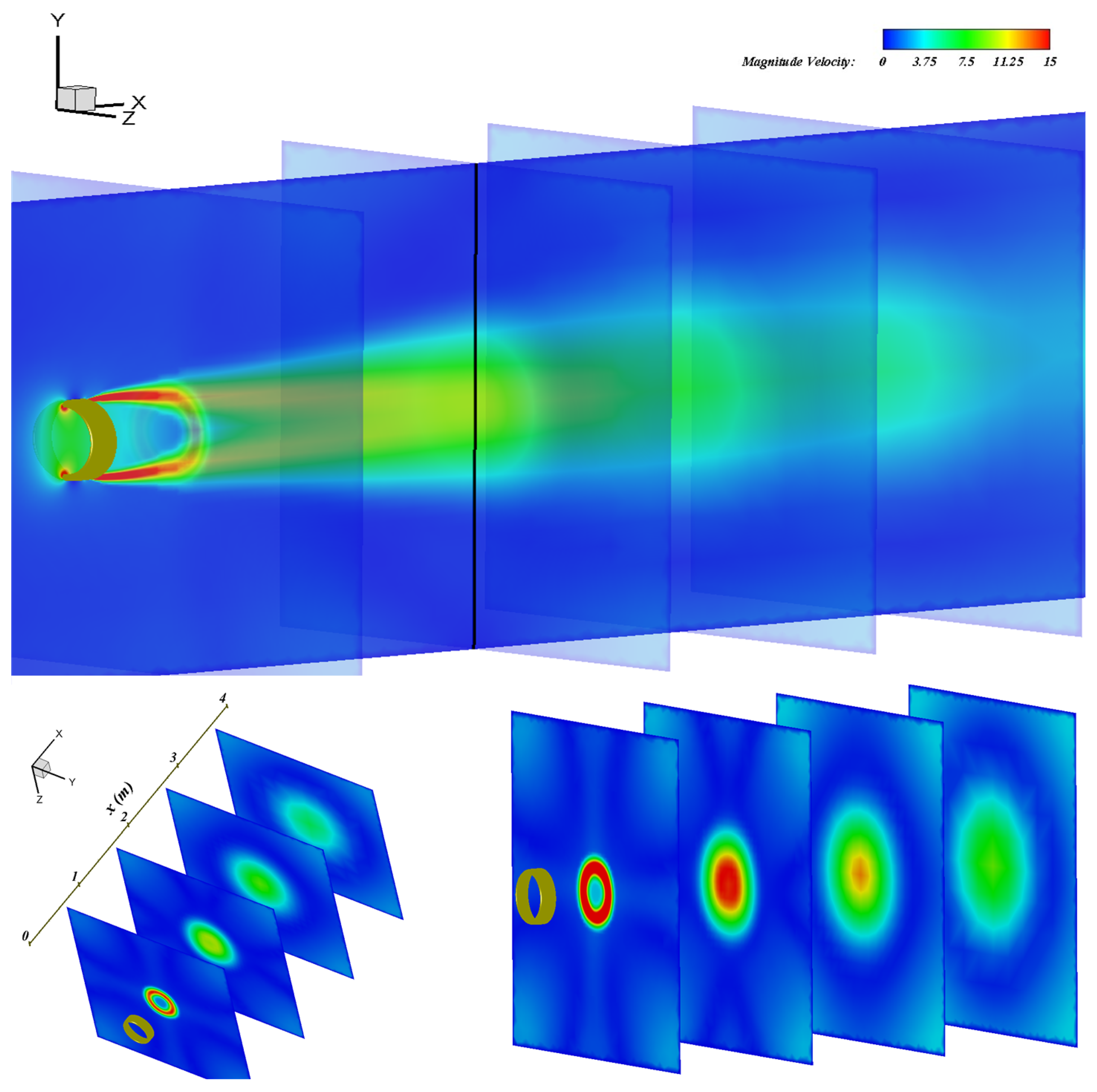
Figure 12 represents the velocity contour and streamlines to depict flow amplification.
Figure 12 illustrates that at planes at distances less than 0.4 m concentrated velocity profiles are formed along the circumference of the fan. This indicates that the velocity is not spread equally along the planar region, which is not ideal. At a distance of 0.4 m, the velocity distribution started to develop. From 0.9 m to 1.8 m, the velocity profile continues to develop. Finally, it attains a uniform distribution at 1.8 m, as seen in
Figure 13. This observation inferred that the optimal occupant distance from the fan is 1.8 m away from the trailing edge.
Figure 14 depicts the velocity distribution of air at a certain distance from the axis. Four lines on the velocity contour plot to analyze the velocity distributions as a function of the y distance on the lines. The four curves on the graph represent each of the planes on the velocity contour diagram. The velocity at the first line (x/D = 0.4 m distance from slit) shows a maximum velocity of 7.5 m/s near the center. The second line from the left (0.9 m distance from slit) has a maximum velocity of around 4.5 m/s, and the third (1.35 m distance from slit) and fourth (1.8 m distance from slit) have velocities of 4.1 m/s and 3.7 m/s, respectively. Thus, the graph plots conclude that at a distance between 0.9 m and 1.8 m, the graph shows a lower and uniform gradient of velocity.
The velocity profile follows a parabolic curve in bladeless fans, with the peak located at the center. The flow develops when the velocity profile contours straighten out after converging at the parabola’s vertex. The flow does not fully develop at a distance of 0.4 m from the fan, which proves that velocity remains higher closer to the circumferential area of the fan. As
Figure 13 suggests, the flow becomes fully developed at a distance of around 0.9–1.35 m from the slit. While it is essential to analyze the velocity distribution of air through contours and graphs, it is also imperative to understand the direction of flow.
Figure 15 represents the direction of airflow using velocity vector plots of the 2 mm slit thickness iterations.
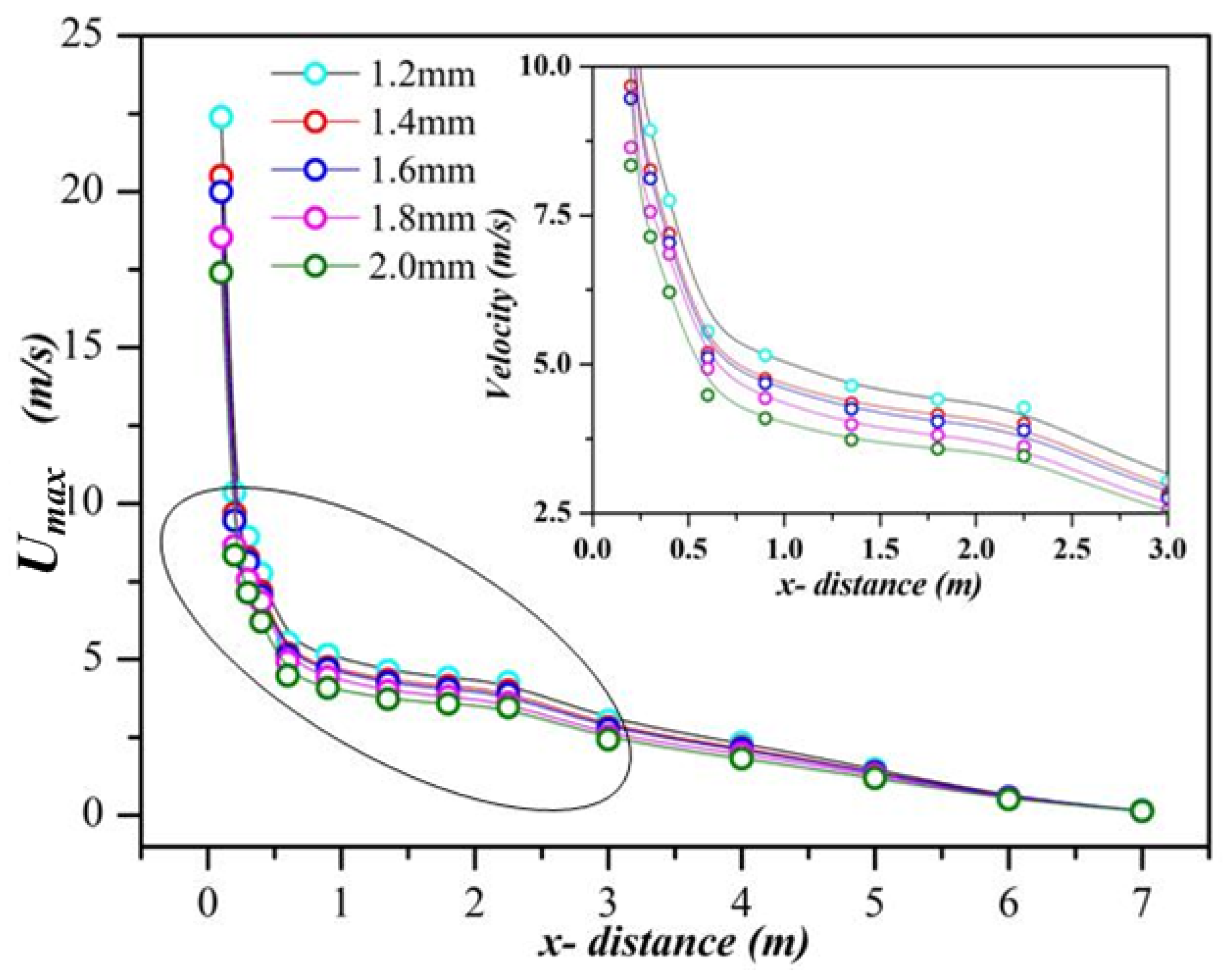
Maximum velocity (U
) at different distances from the slit was observed for various slit thicknesses. The results are in the form of a plot in
Figure 16. At a very close distance from the slit, the velocity is around 20 m/s. As we move from 0.1 m to 0.2 m away from the slit, the maximum velocity drops significantly from 20 m/s to 10 m/s. Furthermore, from 0.2 m to 0.9 m, the velocity drops from 10 m/s to nearly 5 m/s. Finally, the maximum velocity decreases at a stable rate from 5 m/s to 0.143 m/s at distances greater than 1 m from the slit.
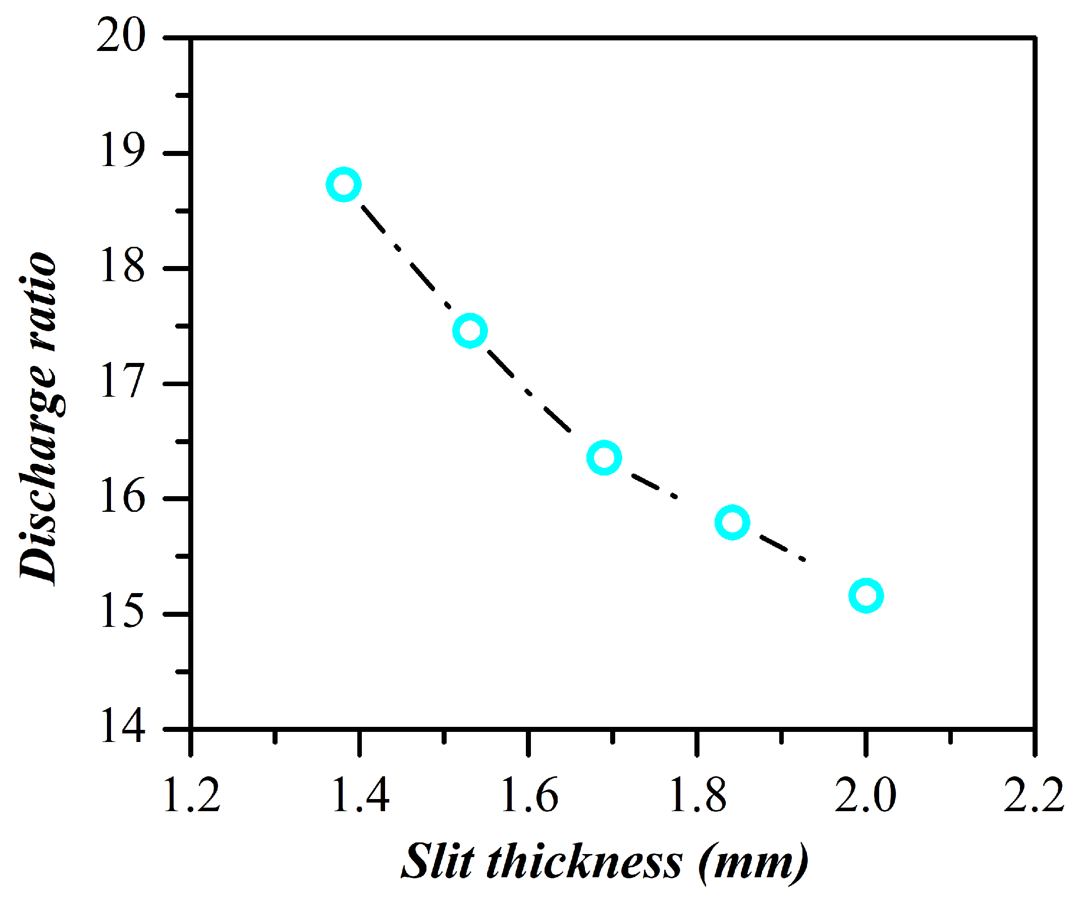
The following graph shows the trend of discharge ratio to slit thickness. Since the inlet velocity is constant for the samples, the outlet velocity increases with a decrease in slit thickness. This increment of velocity due to smaller slit thicknesses increased the discharge ratio substantially. Therefore, the case with a slit thickness of 1.2 mm showed a maximum discharge ratio of 18.784, shown in
Figure 17. Another important observation is that the variation of discharge ratio for the outlet slit thickness is linearly decreasing.
6.4. Variation of Outlet Angle
The outlet slit angle significantly affects the direction of the flow of air. Variation of outlet slit angles changes the distance at which the flow fully develops. In this study, the outlet slit thickness is varied between 16
and 26
with an increment of 2
as shown in
Figure 18a.
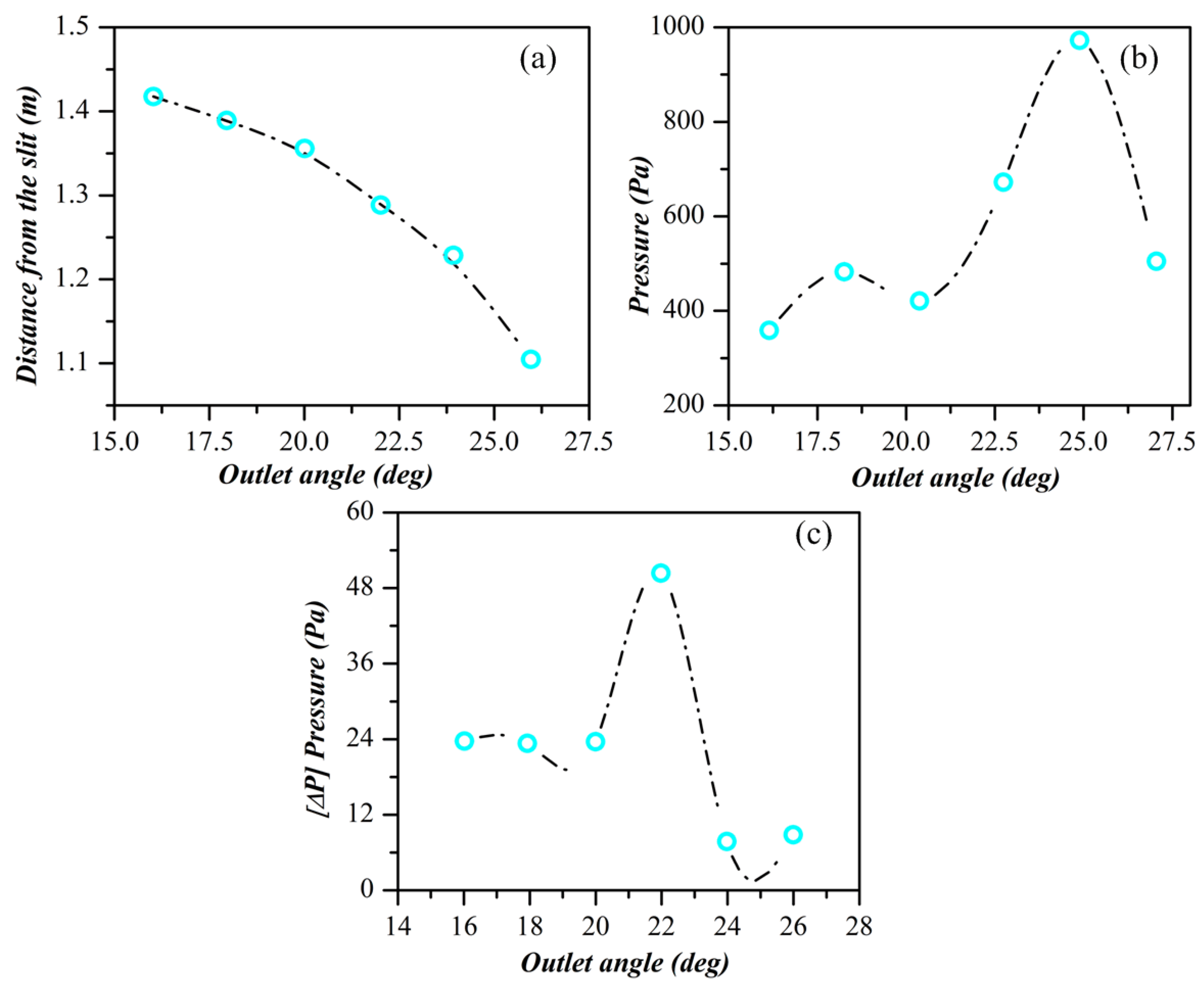
The outlet slit thickness and inlet velocity were 1.2 mm and 3 m/s, respectively. These values were finalized based on previous iterations conducted on outlet slit thickness and inlet velocity variation. Increasing the outlet slit angle reduces the resultant velocity of the air coming out of the fan since a higher outlet slit angle reduces the horizontal component of air velocity. A smaller outlet slit angle increases the converging distance of the fan’s velocity profile, which is undesirable. The velocity profile converging distances of the bladeless fans are plotted against various outlet angles. The graph above shows that an outlet angle of 26
gives a convergence distance of just 1.13 m. Although 26
outlet angle creates a low convergence distance, the steep outlet angle can reduce the Coanda effect along the airfoil. To investigate this, the pressure is measured at the slit, leading edge, and trailing edge. The graph in
Figure 18b below depicts the pressure difference between the slit, and
Figure 18b shows the difference between the leading edge and the trailing edge and leading edge pressures. Theoretically, a greater pressure difference is preferable for increasing the Coanda effect.
Figure 18c infers that the 24
outlet angle shows the greatest pressure drop across the airfoil. The other iterations show a pressure drop of around 300 to 500 Pa. Since the 24
outlet angle shows the highest pressure drop, the Coanda effect will facilitate the most.
Figure 18c shows a slight pressure difference between the trailing edge and the atmosphere for the 24
outlet angle, which means there will be lesser turbulence at the front of the fan, which is suitable for its performance.
7. Conclusions
This study aimed to understand the influence of outlet slit thickness and outlet angle on the performance of the bladeless fan. The two-dimensional analysis fortified the theoretical understanding that outlet velocity increases with a decrease in slit thickness. It was also observed that the velocity profile flattens with distance from the fan. The three-dimensional analysis results shows that the standard deviation of all slits remains almost the same for inlet velocities under 3.3 m/s, and 1.6 mm slit thickness shows the lowest standard deviation of up to 5.4 m/s inlet velocity. For inlet velocities above 2.4 m/s, the 1.2 mm slit has the highest average outlet velocity. This velocity also falls in the range of occupant comfort.
The 1.2 mm slit thickness with 3 m/s inlet velocity was considered the best for the following reasons:
- (i)
The standard deviation is 0.25, which is small and will not cause any discomfort under operational conditions.
- (ii)
At the velocity profile convergence distance, the outlet air velocity will be 4.85 m/s, which is comfortable.
- (iii)
Although other iterations have higher and comparable output velocities at the target distance, the 1.2 mm slit thickness is most favorable because it consumed less energy owing to its lower input velocity.
Velocity contour plots indicated that the flow has a curved profile. The flow begins to develop at 0.9 m from the trailing edge, approximately three times the fan diameter, and fully develops at 1.8 m. The maximum velocity to distance ratio from slit plots suggests that smaller slits show higher maximum velocity throughout the upstream flow. Finally, a comparison of the discharge ratio for different slit thicknesses demonstrated that the discharge ratio decreases linearly with an increase in slit thickness. The decrement of slit thickness from 2 mm to 1.2 mm showed a 24.2% increment in the discharge ratio. The outlet angle affects the pressure difference across the airfoil. A higher pressure difference between the slit and the trailing edge facilitates the Coanda effect. The 24-degree outlet angle shows the highest pressure drop of 965 Pa, while the 16-outlet angle shows just a 355 Pa pressure drop, which is approximately 63% lesser. The 24 outlet does create a huge pressure difference between the leading and trailing edge, thereby reducing the chances of losses due to turbulence. In addition, the velocity profile develops 1.13 m from the trailing edge for the 26 outlet while the 16 outlet flow develops at a distance of 1.4 m.
Author Contributions
V.J.: Modeling and simulation, data visualization, writing of the manuscript. W.N.: Modeling and simulation, data visualization, writing of the manuscript. V.G.: Conceptualization, supervised the findings of the work, results interpretation, and writing of the manuscript. S.R.: Supervised the findings of this work, results interpretation. R.K.B.: Experiment, CFD conceptualization, illustration of results and writing of the manuscript. All authors have read and agreed to the published version of the manuscript.
Funding
This research received no external funding.
Acknowledgments
The authors of this article would like to express gratitude to the School of Mechanical Engineering (SMEC), VIT, for granting access to computational laboratories to carry out this study.
Conflicts of Interest
The authors declare that they have no competing financial interests or personal relationships that could have appeared to influence the work reported in this paper.
Abbreviations
The following abbreviations are used in this manuscript:
| Skin Friction Coefficient |
| L | Characteristic length |
| NACA | National Advisory Committee for Aeronautics |
| Reynolds Number |
| TKE | Turbulence Kinetic Energy |
| Friction velocity |
| U | Freestream Velocity |
| Overall height of the cell adjacent to the boundary layer |
| Wall height adjacent cell to the centroid |
| Non-dimensional wall distance (value-based on turbulence model) |
| Dynamic Viscosity |
| density |
| wall shear stress |
References
- Gammack, P.D.; Nicolas, F.; Simmonds, K.J. Bladeless Fan. U.S. Patent 2009/0060710Al, 13 November 2012. [Google Scholar]
- Jafari, M.; Afshin, H.; Farhanieh, B.; Bozorgasareh, H. Numerical aerodynamic evaluation and noise investigation of a bladeless fan. J. Appl. Fluid Mech. 2014, 8, 133–142. [Google Scholar]
- Jafari, M.; Afshin, H.; Farhanieh, B.; Bozorgasareh, H. Experimental and numerical investigation of a 60 cm diameter bladeless fan. J. Appl. Fluid Mech. 2016, 9, 935–944. [Google Scholar]
- Chunxi, L.; Ling, W.S.; Yakui, J. The performance of a centrifugal fan with enlarged impeller. Energy Convers. Manag. 2011, 52, 2902–2910. [Google Scholar] [CrossRef]
- Quinn, W.R. Upstream nozzle shaping effects on near field flow in round turbulent jets. Eur. J. Mach. B/Fluids 2006, 55, 279–301. [Google Scholar] [CrossRef]
- Aureliano, F.D.; Guedes, L.C. Computational fluid dynamics (CFD): Behavioral study and optimization of the blades number of a radial fan. Procedia Manuf. 2019, 38, 1324–1329. [Google Scholar] [CrossRef]
- Panigrahi, D.C.; Mishra, D.P. CFD simulations for the selection of an appropriate blade profile for improving energy efficiency in axial flow mine ventilation fans. J. Sustain. Min. 2014, 13, 15–21. [Google Scholar] [CrossRef]
- Jeong, S.; Lee, J.; Yoon, J. Optimal nozzle design of bladeless fan using design of experiments. Trans. Korean Soc. Mech. Eng. A 2017, 41, 711–719. [Google Scholar]
- Li, G.; Hu, Y.; Jin, Y.; Setoguchi, T.; Kim, H.D. Influence of Coanda surface curvature on performance of bladeless fan. J. Therm. Sci. 2014, 23, 422–431. [Google Scholar] [CrossRef]
- Sarraf, C.; Nouri, H.; Ravelet, F.; Bakir, F. Experimental study of blade thickness effects on the overall and local performances of a controlled vortex designed axial-flow fan. Exp. Therm. Fluid Sci. 2011, 35, 684–693. [Google Scholar] [CrossRef]
- Ravi, D.; Rajagopal, T.K.R. Numerical Investigation on the Effect of Geometric Shape and Outlet Angle of a Bladeless Fan for Flow Optimization using CFD Techniques. Int. J. Thermofluids 2022, 15, 100174. [Google Scholar] [CrossRef]
- Mohaideen, M.M. Optimization of backward curved aerofoil radial fan impeller using finite element modelling. Procedia Eng. 2012, 38, 1592–1598. [Google Scholar] [CrossRef]
- Raj, D.; Swim, W.B. Measurements of the mean flow velocity and velocity fluctuations at the exit of an FC centrifugal fan rotor. J. Eng. Power 1981, 103, 393–399. [Google Scholar] [CrossRef]
- Krishnaraj, A.; Ganesan, V. Influence of slot profiles on the characteristics of jets. Aircr. Eng. Aerosp. Technol. 2022, 95, 120–131. [Google Scholar] [CrossRef]
Figure 1.
Eppler 473 Airfoil Profile with the depiction of outlet slit and height of cross-section.
Figure 1.
Eppler 473 Airfoil Profile with the depiction of outlet slit and height of cross-section.
Figure 2.
(a) Fluid Domain Boundary Conditions. (b) Airfoil Boundary condition.
Figure 2.
(a) Fluid Domain Boundary Conditions. (b) Airfoil Boundary condition.
Figure 3.
Velocity profile at the downstream of the fan with different values.
Figure 3.
Velocity profile at the downstream of the fan with different values.
Figure 4.
(a) 2D computational domain. (b) Inflation layers near airfoil and outlet slit.
Figure 4.
(a) 2D computational domain. (b) Inflation layers near airfoil and outlet slit.
Figure 5.
(a) 3D Computational domain. (b) Bladeless fan mesh zoomed-view. (c) Inflation layers around the model.
Figure 5.
(a) 3D Computational domain. (b) Bladeless fan mesh zoomed-view. (c) Inflation layers around the model.
Figure 6.
Comparison of downstream velocity validated with Computational by Jafari et al. [
4], and experiment by Quinn [
5].
Figure 6.
Comparison of downstream velocity validated with Computational by Jafari et al. [
4], and experiment by Quinn [
5].
Figure 7.
Reference lines in the 2D domain for measuring properties of fluid flow.
Figure 7.
Reference lines in the 2D domain for measuring properties of fluid flow.
Figure 8.
Velocity Profile and contours (a) 1.2 mm slit thickness at 3 m/s inlet velocity. (b) 2 mm slit thickness at 6 m/s inlet velocity.
Figure 8.
Velocity Profile and contours (a) 1.2 mm slit thickness at 3 m/s inlet velocity. (b) 2 mm slit thickness at 6 m/s inlet velocity.
Figure 9.
Streamline flow distribution 2D (a) 1.2 mm slit thickness at 3 m/s inlet velocity. (b) 2 mm slit thickness at 6 m/s inlet velocity.
Figure 9.
Streamline flow distribution 2D (a) 1.2 mm slit thickness at 3 m/s inlet velocity. (b) 2 mm slit thickness at 6 m/s inlet velocity.
Figure 10.
(a) Average velocity at a distance of 0.9 m from the outlet slit (b) Standard deviation of velocity (U’) at a distance of 0.9 m from the outlet slit (c) Maximum velocity at a distance of 0.9 m from the outlet slit.
Figure 10.
(a) Average velocity at a distance of 0.9 m from the outlet slit (b) Standard deviation of velocity (U’) at a distance of 0.9 m from the outlet slit (c) Maximum velocity at a distance of 0.9 m from the outlet slit.
Figure 11.
Velocity magnitude (m/s) and Turbulent Kinetic Energy (m · s) from the slit (a) 1.2 mm (b) 2 mm thickness.
Figure 11.
Velocity magnitude (m/s) and Turbulent Kinetic Energy (m · s) from the slit (a) 1.2 mm (b) 2 mm thickness.
Figure 12.
Streamline and Velocity contours of 1.2 mm slit thickness (V = 3 m/s).
Figure 12.
Streamline and Velocity contours of 1.2 mm slit thickness (V = 3 m/s).
Figure 13.
Perspective view of airflow at downstream of 1.2 mm slit thickness with 3 m/s inlet velocity.
Figure 13.
Perspective view of airflow at downstream of 1.2 mm slit thickness with 3 m/s inlet velocity.
Figure 14.
Perspective view of airflow downstream of 1.2 mm slit thickness with 3 m/s inlet velocity.
Figure 14.
Perspective view of airflow downstream of 1.2 mm slit thickness with 3 m/s inlet velocity.
Figure 15.
Velocity Vectors displaying the direction of output air in the 3D domain at a distance of 0.9 m from the fan.
Figure 15.
Velocity Vectors displaying the direction of output air in the 3D domain at a distance of 0.9 m from the fan.
Figure 16.
U vs. distance from the slit.
Figure 16.
U vs. distance from the slit.
Figure 17.
Slit thickness vs. Discharge ratio.
Figure 17.
Slit thickness vs. Discharge ratio.
Figure 18.
(a) Converging distance for different outlet angles, (b) Pressure difference between the slit and leading edge for different outlet angles and (c) Pressure difference between the trailing and leading edge for different outlet angle.
Figure 18.
(a) Converging distance for different outlet angles, (b) Pressure difference between the slit and leading edge for different outlet angles and (c) Pressure difference between the trailing and leading edge for different outlet angle.
Table 1.
Details of rid resolution.
Table 1.
Details of rid resolution.
| Grid Name | | No. of Elements (Millions) |
|---|
| Coarse | 15 | 10.2 |
| Basic | 12 | 13.45 |
| Reference | 8 | 14.65 |
| Fine | 6 | 15.4 |
| Disclaimer/Publisher’s Note: The statements, opinions and data contained in all publications are solely those of the individual author(s) and contributor(s) and not of MDPI and/or the editor(s). MDPI and/or the editor(s) disclaim responsibility for any injury to people or property resulting from any ideas, methods, instructions or products referred to in the content. |
© 2023 by the authors. Licensee MDPI, Basel, Switzerland. This article is an open access article distributed under the terms and conditions of the Creative Commons Attribution (CC BY) license (https://creativecommons.org/licenses/by/4.0/).


 ,
, 


