A New Two-Foci V-Trough Concentrator for Small-Scale Linear Fresnel Reflectors

Abstract

We present the design of an original secondary cavity for use in Small-Scale Fresnel Reflectors in photovoltaic applications. The cavity is similar to the classical V-trough, but the primary reflector system is configured so that there are two focal points on the aperture. The rays coming from each side of the primary system reach the opposite side of the cavity, producing a non-symmetrical distribution of the irradiance. This modifies the acceptance half-angle and allows us to break the maximum limit for the concentration ratio of ideal symmetric concentrators. Our study is analytic, and we provide formulas for any number of reflections. Numerical simulations with a ray-tracing program based on MATLAB are included. We provide a comparison of optical concentration ratio, height and cost parameter between our system and two classical designs with a single focal point: the V-trough and the Compound Parabolic concentrators. This way, we verify that our design yields better concentration ratios while keeping the ray acceptance rate at one. Our solution proves to be better than both the classical one-focus V-trough and the Compound Parabolic concentrator. Specifically, the proposed solution is significantly better than the classical one-focus V-trough in optical concentration ratio, with an increase between $15.02$ and $35.95$%. As regards the compound parabolic concentrator, the optical concentration ratio is always slightly better (around $4\%$). The height of the cavity, however, is notably less in this design (around $54.33\%$).

1. Introduction

Human activity is the greatest source of greenhouse gas (GHG) emissions, as fossil fuels are the main energy source for these activities: hence, the emergence of the term Anthropocene to describe the human modification of the Earth’s climate [1]. This has led to the organization of international meetings between representatives of most countries, the so-called Conferences of Parties (COP). At the last meeting (COP27), in Egypt in 2022, attended by 196 countries plus the European Union as a whole, stringent decisions to reduce global greenhouse gas emissions were supported [2].

Renewable energies are possibly the main solution to GHC emissions. In particular, decentralised energy systems with storage systems [3] give hope to meet the challenge [4].

Photovoltaic systems are one of the main solar energy technologies used to avoid climate change. A typical application of this technology is concentrator photovoltaic (CPV) systems. They can be grouped in three classes, according to what is called their geometric concentration ratio: the ratio between the area of the lens or primary mirror and the area of the PV cells. The classes are: low, medium and high concentration [5] systems. This work will focus on low concentration photovoltaic (LCPV) systems with a geometric concentration coefficient between 2 and 10 suns.

Among the types of concentrators used in the design of LCPVs [6], this work will focus on the small-scale linear Fresnel reflector (SSLFR). In addition to having a lower manufacturing cost than other solar concentrators, they showcase a well-proven technology that has been the subject of multiple studies (see [7,8,9,10], for instance). These reflectors concentrate the sunlight onto a secondary system by means of a row of longitudinal mirrors.

The geometric concentration ratio [11,12] of an SSLFR is a critical measure of its efficiency, especially when solar cells are used. Systems with a higher concentration ratio allow for less (or smaller) cells and prevent complications in the design of the primary field: the lower the concentration ratio, the thinner the mirrors must be, which makes the system either costlier or more difficult to maintain, or both (more mirrors are needed, hence more movable parts, etc.). Another important effect to avoid is a heterogeneous distribution of the flux of light [13], which causes inefficiencies and may lead to the appearance of hotspots, which can even lead to the total failure of the system as long as they persist.

Many concentration methods [14] have been proposed to improve the yield of solar systems. They can be divided in two large categories: nonimaging concentrators (which do not produce clearly defined images of the Sun on the absorber) and imaging ones (which form clear images). The former reflect all of the incident radiation towards the receiver as long as the incidence angle remains in a specific range (acceptance angle). The most important example of these systems is the compound parabolic concentrator (CPC). Nonimaging concentrators are usually the most appropriate for use in solar concentration (v.gr. concentrated photovoltaic systems). Imaging concentrators (such as parabolic reflectors or Fresnel lenses), for their part, provide wider acceptance angles, higher tolerances for imperfections and errors, higher solar concentrations, more uniform illumination of the receiver and greater design flexibility.

Madala and Boehm [15] provide a thorough review of solar concentrators, including the large family of CPCs (with different reflector and absorber geometries), Fresnel mirrors, V-trough concentrators, etc. Some conventional imaging type concentrators (such as parabolic troughs) are also covered in their study. More recent designs can be found in [16] (v.gr. concentrators with multi-surface and multielement combinations). As we propose a modification of the classical V-trough concentrator, we are only going to review this one.

Duffie [17] is one of the main references in this area: the acceptance angle (the angle such that any incident ray forming a lesser angle with the cavity gets to the absorber) is introduced in that work. He approximates the system using the tangents to a reference circle passing through one of the end points of the aperture. That reference [17] also contains the study of linear, two-dimensional, V-trough concentrators. He studies a system with two flat plate reflectors, an ideal concentrator perfectly aligned with the Sun and with a single reflection. V-trough concentrators have been considered the best in terms of uniformity of flux distribution [18]; their reduced complexity and lower manufacturing costs [19] also make them very convenient.

There is a good amount of literature on V-trough concentrators for different applications. Shaltout et al. [20] evaluated a V-trough concentrator on a photovoltaic system with two-axis solar tracing in a hot desert climate. Their system, which has a concetration ratio of $1.6$, generates $40\%$ more PV power than the same system without a concentrator. Different concentrator geometries, depending on the incidence angle of the solar irradiation as well as the effect of the wall angle of the trough, are considered by Solanki et al. [21], Maiti et al. [22], Chong et al. [23], Tina and Scandura [24], Singh et al. [19] and Al-Shohani et al. [25]. Recently, Al-Najideen et al. [26] proposed a new design by adding two additional elements to the Hollands concentrator, resulting in four symmetrical reflectors surrounding the PV cell. They call their design “Double V-trough Solar Concentrator”. Our proposal follows their spirit, as we provide a new modification, specifically designed for SSLFR systems: a V-trough with two foci.

The optical behaviour of the cavity can be described using the method of images applied to V-trough linear concentrators by Duffie [17]. Other papers also present optimal designs of concentrators using analytical solutions of the equations describing the number of reflections of rays through the trough [27]. Fraidenraich [18,28,29] used the method of images, with an additional condition on the design (the illumination of the module’s surface has to be uniform) to describe the optical behaviour of the class of V-trough cavities. More recently, Tang [30] presented a detailed mathematical procedure for the design of a V-trough concentrator with attached solar cells. The solution is found using the method of images and determining the fraction of solar rays arriving at the cells after any number of reflections.

Another widely used approach uses ray-tracing techniques in order to design, simulate and optimize different types of V-trough concentrators. For instance, Chong et al. [23] use this technique implemented in Microsoft Visual C++. Maiti et al. [22] use Monte Carlo ray-tracing, as does Paul [31]. Narasimman and Selvarasan [32] use the software Trace-Pro to simulate. Finally, Hadavinia y Singh [33] use Comsol.

The concentration ratio of V-trough concentrators depends on the acceptance half-angle ${\theta }_c$: the largest incidence angle for which no radiation is rejected. When the design of the system is symmetric and the distribution of irradiance going into the concentrator is uniform for any $\theta$ with $\left|\theta \right|\le \left|{\theta }_c\right|$, it is well-known [17] that a two-dimensional (linear) concentrator (such as the V-trough) has a concentration ratio bounded by $C_{ideal}^{2D}={sin}^{-1}{\theta }_c$. In our design, we take advantage of the nature of an SSLFR in order to develop a configuration of the primary reflector system which gives rise to a non-uniform distribution of the irradiance on the cavity with two different focal points, so that each side of the SSLFR is focused on one of them.

As explained above, many authors have tried to determine the acceptance rate ${\eta }_{ray}$ using both analytical and statistical methods. We have a different objective: to maximize the concentration ratio under the condition ${\eta }_{ray}=1$ for all the incidence angles less than the acceptance half-angle ${\theta }_c$. We do not use the method of images, only planar mirror geometry, and we compute the optimal design using closed-form analytic methods. In our study, we can analyze any number of reflections. The advantage over ray-tracing is obvious: we provide a universal method for computing the optimal design, regardless of simulations.

The inspiration for this new design comes from a previous study by some of the authors [34]. In that paper, dedicated to the application of SSLFRs to illumination by means of optic fiber, two non-symmetrical trapezes were joined along their vertical side, in order to construct what can be called a “half-trough concentrator”. From the design and the specific functioning of the SSLFR, the reflected rays reach each of the two cavities from the corresponding side of the primary field. That way, light from a wider inlet aperture was concentrated into a narrower area (the absorber). What we have realized is that this design can be improved, removing the vertical wall but keeping the two different foci of the (previous) cavities. This reduces the number of reflections required for a ray to reach the absorber area (by a little less than one-half), and the amount of material required to build the concentrator. Thus, we both improve the efficiency and reduce costs. Furthermore, we carry out the whole theoretical study with analytical solutions in this paper, whereas in [34] only simulations with Maltab were performed.

Each focus of the receiver cavity is reached by rays satisfying the requirement $\theta \le {\theta }_c$ on each side. These conditions are weaker than the global condition $\left|\theta \right|\le |{\theta }_c|$, the one governing the usual one-focus half-trough design. The breakthrough is that this change of condition for the acceptance angle provides a concentration ratio greater than the one for symmetric concentrators with uniform irradiance distribution (one focal point)namely $C_{ideal}^{2D}$, and this happens for any acceptance half-angle. As far as we know, there is no such result in the literature.

All the previous literature covers the single-focus V-trough concentrator and the compound parabolic concentrator. We have not found any reference dealing with a double-foci V-trough concentrator.

Thus, the aim of this work is very specific. Starting from a two-focus configuration that causes a non-symmetric distribution of irradiance at the secondary reflector aperture, the cavity will be designed with the following property: it must maximise the geometrical concentration ratio under the condition that the ray acceptance rate is equal to one for all angles of incidence less than the half-angle of acceptance.We do not impose any restriction on the height of the cavity.

The specific contributions of this study can be summarized in the following proposals:

(i)

We propose a secondary cavity prepared for low-concentration photovoltaic systems based onSSLFRswith a large concentration ratio and non-uniform solar irradiance distribution.

(ii)

The design obtains a concentration ratio greater than the maximum possible for systems with uniform irradiance distribution [17].

The paper is organized as follows: Section 2 contains the basic notions about concentrators. A brief description of the SSLFR for concentration PV applications with the two-foci design and the geometric design of the two-foci V-trough concentrator is given in Section 3. Section 4 includes numerical results and validations of the proposed design, which is compared with other classical concentrators (CPC and V-trough) in Section 5. Finally, Section 6 contains a summary of the main conclusions.

2. Main Parameters of a Concentrator

Duffie [17] states the fundamental problem in the design of concentrators as follows: “How can radiation which is uniformly distributed over a range of angles $\left|\theta \right|\le \left|{\theta }_c\right|$ and incident on an aperture of area $A_a$, be concentrated on a smaller absorber area $A_{abs}$, and what is the highest possible concentration”. He is using the most common definition of concentration ratio, the area or geometric concentration ratio:

$$C_a=\frac{\mathrm{aperture} \mathrm{area}}{\mathrm{absorber} \mathrm{area}}=\frac{A_a}{A_{abs}}$$

(1)

Notice that in his statement, he assumes that the radiation is uniformly distributed (and uniformly reflected). From this hypothesis, it follows that this ratio has an upper limit which depends on whether the concentrator is three-dimensional (spherical) or a two-dimensional (linear) concentrator, such as our V-trough design. From the Second Law of Thermodynamics, Rabl concludes that the maximum possible concentration ratio for a given acceptance half angle ${\theta }_c$ is:

$$C_{ideal}^{2D}={sin}^{-1}{\theta }_c$$

(2)

For two-dimensional (trough-like) concentrators, as he remarks, a concentrator is ideal if and only if the exchange factor that measures the radiation going from absorber to the source is one. It is known that compound parabolic concentrators (CPC) actually reach this limit, so that they have been called “ideal concentrators” [17].

In addition to this index, there are other indices that measure the goodness of a concentrator, such as the flux concentration ratio. It is defined as the ratio of the average energy flux on the receiver to that on the aperture; the local flux concentration ratio which is the ratio of the flux at any point on the receiver to that on the aperture and which varies across the receiver. In order to avoid confusion, we will use the following notation (commonly used in the literature, e.g., in [24,25] or [33]):

$$C_{opt}=\frac{\mathrm{flux} \mathrm{at} \mathrm{the} \mathrm{receiver}}{\mathrm{flux} \mathrm{at} \mathrm{the} \mathrm{absorber}}=C_a·{\eta }_{ray}$$

(3)

where $C_{opt}$ is the optical concentration ratio, $C_a$ is the area concentration ratio, and ${\eta }_{ray}$ is the ray acceptance rate, defined as the fraction of incident light rays reaching the absorber.

Duffie [17] presented the following equation for the classical “single-focus” (so to say) V-concentrator, considering: ideal concentrator, perfectly aligned with the Sun, and with a single reflection:

$$C_a=1+2cos\left(2\mathsf{\Phi }\right)$$

(4)

where $\mathsf{\Phi }$ is the trough angle or half angle of the V-shaped cone. Equation (4) has also been used by [24]. Duffie [17] also used the concept of the half angle of the V-shaped cone, obtaining the following equation:

$$C_a=\frac{1}{sin({\theta }_c+\mathsf{\Phi })}$$

(5)

Equation (5) has also been used by [15].

Fraidenraich [28] presented a paper in which he showed that the optical concentration ratio can be approximated by a function of two parameters: the ray acceptance rate and the average number of reflections, n. In Fraidenraich [18], the main hypothesis is the condition of uniform illumination of the absorber’s surface within an angular interval of light incidence. Using it, he provides analytical expressions relating $C_a$ and $\mathsf{\Phi }$ and also a cost analysis. Tang [30] presents a study where he considers $\mathsf{\Phi }$ and $C_a$ as independent parameters that determine the geometry of a V-trough concentrator. Rabl [35] shows that slight errors in the calculation of n are almost irrelevant on the final value of ${\rho }_m^n$.

Finally, thereflector-to-aperture area ratio parameter is defined:

$$R_a=\frac{\mathrm{reflector} \mathrm{area}}{\mathrm{aperture} \mathrm{area}}=\frac{A_r}{A_a}$$

(6)

It can be intuited that the height of the cavity plays a key role. The $R_a$ parameter is necessary for cost analysis. For example, the high efficiency of ideal CPC concentrators has as a negative trade-off their high $R_a$.

3. Design of a Two-Foci V-Trough Concentrator

In this section, we provide a detailed description of the optimal design of the two-foci V-trough cavity, using analytical formulas exclusively.

3.1. Brief Description of the SSLFR with Two-Foci V-Trough

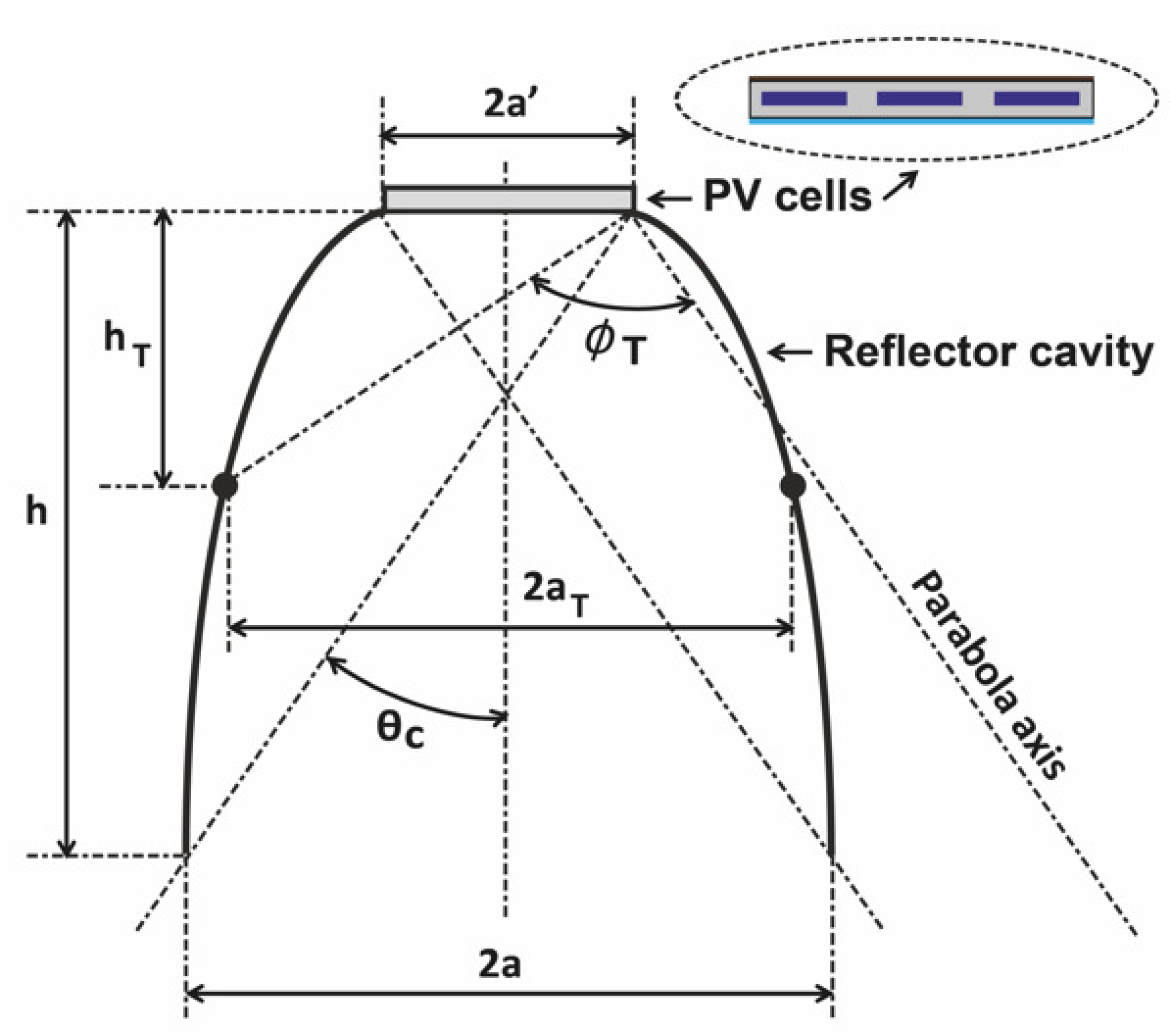
An SSLFR consists of a set of flat mirrors (the primary reflector system) concentrating the direct solar irradiance onto an element with much smaller area which, in our case, is a row of PV cells. The primary reflector system contains a set of parallel stretched mirrors mounted on a frame; in order to follow the Sun’s motion, in our design, each mirror can rotate in the north–south axis. A secondary reflector system—a reflective cavity— is positioned so that the irradiance reflected from the primary system, which does not fall directly on the PV cells, is reflected again and directed towards them.

Figure 1 shows the schematics of the SSLFR: notice the symmetry of the system (except for the orientation of the mirrors). Its main constructive magnitudes are: mirror width ($W_M$), height to the receiver (f), separation between two consecutive mirrors (d), distance from the mirror centers to the center of SSLFR ($L_i$), width of the PV cells (b), aperture of the secondary reflector system (the V-trough cavity) (B) and number of mirrors on each side of the SSLFR ($N_r=N_l$, which we will call N, as we assume the same number of mirrors on each side). The secondary cavity is symmetric with respect to the central axis, but there are two different focal points for the optical system: $F_1$ and $F_2$, one on each side.

For each side of the SSLFR, the angle between the vertical line through the focal point and the line connecting this point with the center of the i-th mirror is:

$${\beta }_i=arctan\frac{L_i}{f}; 1\le i\le N$$

(7)

The maximum ${\beta }_i$ on each side (that is, ${\beta }_{N_r}={\beta }_{N_l}$) is the acceptance angle of the secondary cavity:

$${\theta }_c={\beta }_N$$

(8)

Finally, notice that we are not fixing (at all) the height of the secondary cavity (H, as we will see later): in fact, this is one of the most important variables in our design, as a large value implies a big concentrator, which is undesirable.

3.2. Two-Foci V-Trough Reflector

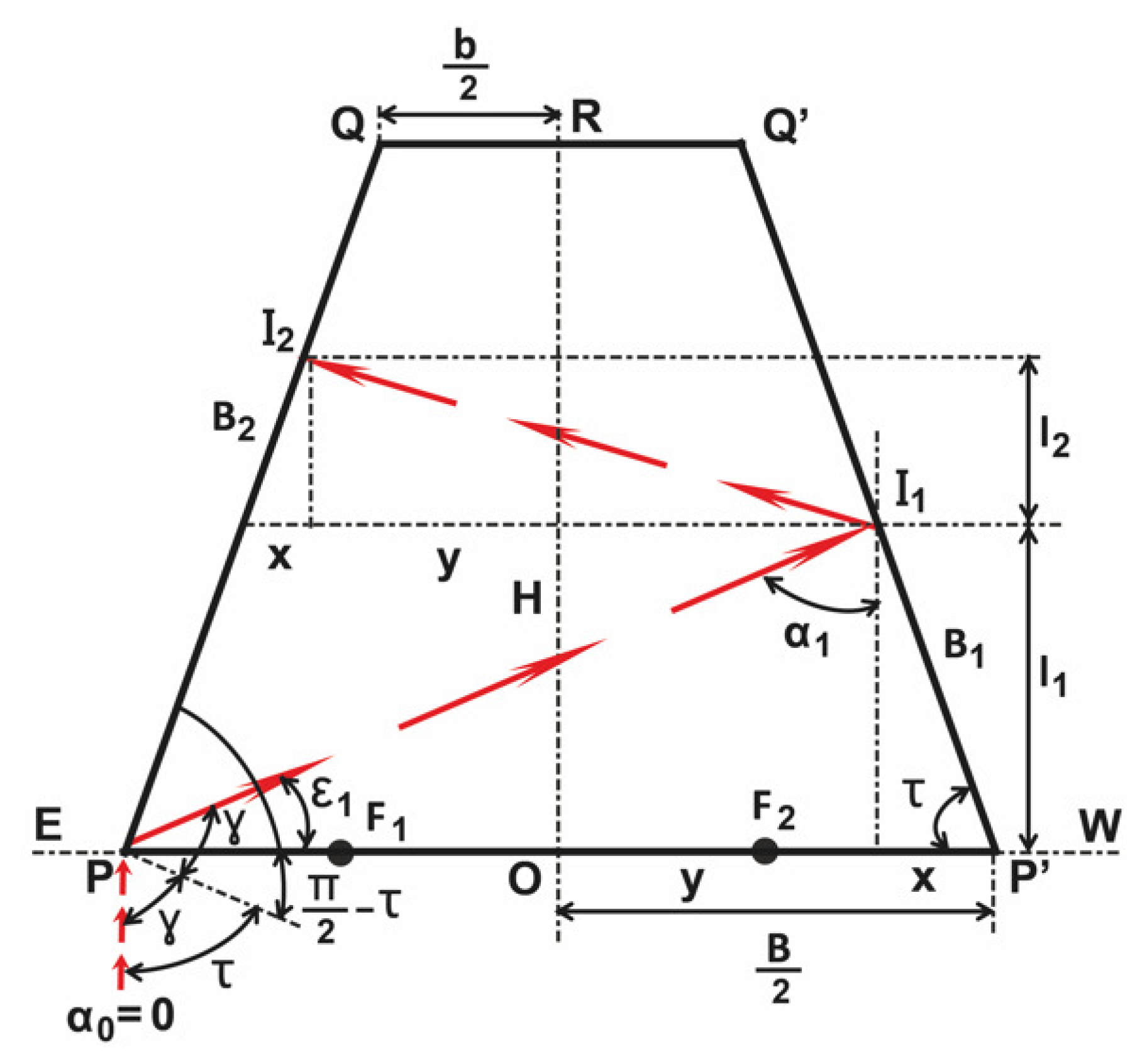
Consider a classical V-trough cavity such as the one depicted in Figure 2. There are two linear side walls ($PQ$ and $P^{\prime }{Q}^{\prime }$) which concentrate light from the wider inlet opening $P{P}^{\prime }$ towards the narrower absorber area $Q{Q}^{\prime }$. Four parameters are considered in this study: the incidence angle of each ray ${\theta }_i$ on the cavity aperture B, the height H of the cavity and the trough wall angle $\tau$. Note that the upper width $QQ\prime$ of the cavity is not a free parameter but a constraint because it is equal to the width of the PV cells. Notice that our angle $\tau$ is the complement of Hollands’ and Rabl’s $\mathsf{\Phi }$. The central axis $OR$ will be the reference axis for angles, and we will consider ${\theta }_i$ to be positive for rays coming from the left side and negative for those coming from the right. Using the notation of Figure 2:

$${\theta }_i={\alpha }_0$$

(9)

For simplicity, we will denote the angle between the ray reaching the cavity and $OR$ as ${\alpha }_0$ (i.e., ${\alpha }_0={\theta }_i$), and each of its successive reflections will be ${\alpha }_j$, for $j=1,2,\dots$

As already stated, the key to our design is to assume that on each side of the concentrator only the rays coming from the same side of the primary reflector system arrive, each with an incidence angle ${\theta }_i$. The position and orientation of the mirrors of the primary field create two focal points $F_1$ and $F_2$, one for each set of mirrors on each side of the field; the left $F_1$ and $F_2$ are on the midpoint of each of the half-bases of B. For simplicity, we will speak of the right and left sides of the cavity, separated by the axis $OR$ despite there being no physical separation.

Of course, our design still aims at computing an acceptance angle ${\theta }_c$ such that the ray acceptance rate ${\eta }_{ray}$ is one, and thus $C_{opt}=C_a$. However, we do not impose the classical condition $\left|{\theta }_i\right|\le \left|{\theta }_c\right|$, but instead:

$$\begin{array}{cc}0\le {\theta }_i\le {\theta }_c\hfill & \mathrm{on} \mathrm{the} \mathrm{left} \mathrm{side} \mathrm{of} \mathrm{the} \mathrm{cavity}\hfill \\ 0\ge {\theta }_i\ge -{\theta }_c\hfill & \mathrm{on} \mathrm{the} \mathrm{right} \mathrm{side} \mathrm{of} \mathrm{the} \mathrm{cavity}\hfill \end{array}$$

(10)

We will only state the left-side case (with rays coming from the right of the SSLFR focused on $F_1$). In these terms, the problem can be stated as: given b, in order to find the maximum $C_a$, we will maximize B under the restriction that all the rays reaching $P{P}^{\prime }$, after a number of reflections, get to the PV cell (whose width is b), that is ${\eta }_{ray}=1$:

$$max{C}_a=maxB; 0\le {\theta }_i\le {\theta }_c$$

(11)

The following property is key to finding the optimal design.

Property 1. 

In order to achieve (11), the optimal solution of the most unfavorable case is that in which the vertical component of each reflection on the walls (if there are any) is largest and touches the base b either on Q or $Q^{\prime }$.

We make use of Property 1, forcing the reflected rays to be as high as possible and to reach the corners Q or $Q^{\prime }$ of the basis b. However, we are no longer in a symmetric geometry, and we have two different cases to consider (see Figure 2 and Figure 3):

$$\begin{array}{cc}\hfill \mathrm{Case} \mathrm{A}& : \mathrm{ray} \mathrm{passing} \mathrm{through} O \mathrm{with} {\theta }_i={\theta }_c;\hfill \\ \hfill \mathrm{Case} \mathrm{B}& : \mathrm{ray} \mathrm{falling} \mathrm{on} P \mathrm{with} {\theta }_i=0.\hfill \end{array}$$

If we make these two rays reach b, any other ray will also, and usually with less reflections. From Figure 2 and Figure 3, one can obtain the formulas for each number n of reflections.

Let us study each of the cases A and B separately.

3.2.1. Case A

Using the Law of Reflection, if n is the number of reflections required to reach the PV cells and starting at ${\theta }_i={\alpha }_0$, the following equalities follow (see Figure 2):

$${\alpha }_1=(\pi -2\tau )+{\alpha }_0; {\alpha }_2=(\pi -2\tau )+{\alpha }_1; \cdots ; {\alpha }_n=(\pi -2\tau )+{\alpha }_{n-1}$$

(12)

As for the angle between $P{P}^{\prime }$ and the $i-$th reflection, called ${\epsilon }_j$:

$${\epsilon }_1=(2\tau -\pi /2)-{\alpha }_0; {\epsilon }_2=(2\tau -\pi /2)-{\alpha }_1; \cdots ; {\epsilon }_n=(2\tau -\pi /2)-{\alpha }_{n-1}$$

(13)

Finally, the vertical lengths traveled by the reflected ray $l_i$ after each reflection are given by the following equations:

For $i=1$ we obtain:

$$l_1={\displaystyle \frac{B/2}{cot\tau +tan{\alpha }_0}}$$

(14)

For the following ones:

$$\begin{array}{cc}{l}_2={\displaystyle \frac{B-2\left(l_1\right)cot\tau }{cot\tau +tan{\alpha }_1}}; l_3={\displaystyle \frac{B-2(l_1+l_2)cot\tau }{cot\tau +tan{\alpha }_2}};\cdots \hfill & \\ & \hfill \cdots ; l_n={\displaystyle \frac{B-2{\sum }_{i=1}^{n-1}\left(l_i\right)cot\tau }{cot\tau +tan{\alpha }_{n-1}}}\end{array}$$

(15)

We now have the tools required for describing the algorithm which gives the optimal design (11). The nested structure of the formulas leads to an easily implementable method.

Where n is the number of reflections on the lateral walls, the algorithm considers different cases $A_n$, depending on n. The height $H_n$ of the cavity for n reflections is:

$$H_n\left(B\right)={\sum }_{i=1}^n{l}_i$$

(16)

substituting into

$$B=b+2H_n\left(B\right)cot\tau$$

(17)

and solving for B, we obtain:

$$\begin{array}{cc}\hfill A_1& :B_1\left(\tau \right)=b+bcot\left({\alpha }_0\right)cot\left(\tau \right)\hfill \\ \hfill A_2& :B_2\left(\tau \right)=-bcos({\alpha }_0-3\tau )csc\left({\alpha }_0\right)csc\left(\tau \right)\hfill \\ \hfill A_3& :B_3\left(\tau \right)=bcos({\alpha }_0-5\tau )csc\left({\alpha }_0\right)csc\left(\tau \right)\hfill \\ \hfill & \cdots \hfill \\ \hfill A_n& :B_n\left(\tau \right)={(-1)}^{n-1}bcos({\alpha }_0-(2n-1)\tau )csc\left({\alpha }_0\right)csc\left(\tau \right)\hfill \end{array}$$

(18)

The case $n=1$ has no physical meaning, as $B\to \infty$ when $\tau \to 0$. The rest of the cases are possible, though. The algorithm finishes by maximizing, using numerical methods, the transcendental equations for $B_n\left(\tau \right)$, thus finding the optimal design angles ${\tau }_n^{*}$ which give the maximal $C_a$. Some qualitative properties can be deduced:

(i)

The optimal value of ${\tau }_n^{*}$ increases with n, and ${\tau }^{*}\to {90}^{°}$ as $n\to \infty$.

(ii)

The optimal value for $C_a$ is reached for $n=3$ ($A_2$) and decreases afterwards asymptotically towards (2).

For each case $A_n$, the number of reflections is $n-1$. We will see this in detail in the next section when we show the example.

3.2.2. Case B

In this case, we just need to set ${\theta }_i={\alpha }_0=0$ in Formulas (12) and (13) to obtain (see Figure 3):

$${\alpha }_1=(\pi -2\tau ); {\alpha }_2=(\pi -2\tau )+{\alpha }_1; \cdots ; {\alpha }_n=(\pi -2\tau )+{\alpha }_{n-1}$$

(19)

$${\epsilon }_1=(2\tau -\pi /2); {\epsilon }_2=(2\tau -\pi /2)-{\alpha }_1; \cdots ; {\epsilon }_n=(2\tau -\pi /2)-{\alpha }_{n-1}$$

(20)

However, the vertical lengths $l_i$ of the $i-$th reflected ray are different from Equation (15). The vertical lengths traveled by the reflected ray $l_i$ after each reflection are given by:

$$\begin{gathered} l_1={\displaystyle \frac{B}{cot\tau +tan{\alpha }_1}}; l_2={\displaystyle \frac{B-2\left(l_1\right)cot\tau }{cot\tau +tan{\alpha }_2}}; l_3={\displaystyle \frac{B-2(l_1+l_2)cot\tau }{cot\tau +tan{\alpha }_3}}; \cdots \hspace{1em}\hspace{1em}\hspace{1em}\hspace{1em}\hspace{1em}\hspace{1em}\hspace{1em}\hspace{1em}\hspace{1em} \\ \hspace{1em}\hspace{1em}\hspace{1em}\hspace{1em}\hspace{1em}\hspace{1em}\hspace{1em}\hspace{1em}\hspace{1em}\hspace{1em}\hspace{1em}\hspace{1em}\hspace{1em}\hspace{1em}\cdots ; l_n={\displaystyle \frac{B-2{\sum }_{i=1}^{n-1}\left(l_i\right)cot\tau }{cot\tau +tan{\alpha }_n}} \end{gathered}$$

(21)

Reasoning as above, stating each case $B_n$ and substituting the height $H_n$

$$H_n\left(B\right)={\sum }_{i=1}^n{l}_i$$

(22)

into:

$$B=b+2H_n\left(B\right)cot\tau$$

(23)

and solving for B, we obtain:

$$\begin{array}{cc}\hfill B_1& :B_1\left(\tau \right)=b\left(1-2cos\left(2\tau \right)\right)\hfill \\ \hfill B_2& :B_2\left(\tau \right)=b\left(1-2cos\left(2\tau \right)+2cos\left(4\tau \right)\right)\hfill \\ \hfill B_3& :B_3\left(\tau \right)=b\left(1-2cos\left(2\tau \right)+2cos\left(4\tau \right)-2cos\left(6\tau \right)\right)\hfill \\ \hfill & \cdots \hfill \\ \hfill B_n& :B_n\left(\tau \right)=b\left(1-2{\sum }_{i=1}^n{(-1)}^{i}cos\left(2i\tau \right)\right)\hfill \end{array}$$

(24)

First of all, notice that this family of functions does not depend on ${\alpha }_0={\theta }_c$. Secondly, and as the main result, when increasing the number of reflections n, we obtain a family of functions whose maximum (without physical meaning) is the asymptotic value:

$$max{B}_n\left(\tau \right)=\underset{\tau \to {90}^o}{lim}{B}_n\left(\tau \right)$$

(25)

As a consequence, the concentration ratios $C_a$ tend to

$$lim{C}_a=3,5,7,\dots$$

(26)

as we increase the number of reflections $n=1,2,\dots$ (obviously, allowing for $H_n\to \infty$).

We think it is remarkable that the classical formula of Hollands for an ideal concentrator which is perfectly aligned with the Sun and with a single reflection:

$$C_a=1+2cos\left(2\mathsf{\Phi }\right)$$

(27)

is just a particular case of our family $B_n\left(\tau \right)$: specifically, $B_1\left(\tau \right)$, as one can verify readily because $\mathsf{\Phi }=\pi /2-\tau$. As a consequence, our study generalizes to any number of reflections the case of an ideal concentrator (perfectly aligned with the Sun).

From the above, it follows that the aim of this case B is no longer to maximize the function $B_n\left(\tau \right)$ but to choose the optimal solutions among the “candidate solutions” $A_n$.

To this end, we need to obtain the general expressions for the heights of the cavity in each case $B_n$. The simplest way is to use:

$$H_n=\frac{B_n-b}{2}tan\left(\tau \right)$$

(28)

which gives:

$$\begin{array}{cc}\hfill B_1& :H_1\left(\tau \right)=-bcos\left(2\tau \right)tan\left(\tau \right)\hfill \\ \hfill B_2& :H_2\left(\tau \right)=-b(cos\left(2\tau \right)-cos\left(4\tau \right))tan\left(\tau \right)\hfill \\ \hfill B_3& :H_3\left(\tau \right)=-b(cos\left(2\tau \right)-cos\left(4\tau \right)+cos\left(6\tau \right))tan\left(\tau \right)\hfill \\ \hfill & \cdots \hfill \\ \hfill B_n& :H_n\left(\tau \right)=-btan\left(\tau \right){\sum }_{i=1}^n{(-1)}^{i-1}cos\left(2i\tau \right)\hfill \end{array}$$

(29)

As the value of b is fixed, using the envelope of this family of curves $H_n\left(\tau \right)$, for each value of $\tau$ we obtain the largest height under the condition ${\eta }_{ray}=1$. This way it becomes easier to verify if the optimal candidate solutions (the values ${\tau }_n^{*}$ and $H\left({\tau }_n^{*}\right)$) computed for the cases $A_n$ also satisfy this case B. The example provided in Section 5 clarifies this step.

The process can be made as long as desired, and we can choose the optimal design depending on the number of reflections n. Qualitatively, the main result is that the larger n is, the larger $B_n$ is, so that $C_a$ increases as well. Actually, $C_a$ tends asymptotically to the ideal value (2).

3.3. Number of Reflections in the Two-Foci V-Trough

Finally, in order to compute the approximate value of n, we will use the property proved by Rabl [35] that the average number of reflections in a V-trough is essentially the same as those in a CPC. Thus, we consider a truncated CPC with the same height as our two-foci V-trough, starting with a whole CPC designed for the specific value of ${\theta }_c$.

We must not forget that the influence of n on the factor ${\rho }_m^n$ is rather small because ${\rho }_m$ is always very near to one.

4. Numerical Results and Validation

In this section, we present an example in order to clarify the method and also as a verification of our results. We set $b=10$ (cm) and ${\theta }_c={\alpha }_0={30}^{°}$ (the acceptance angle), a plausible value for the typical dimensions of an $SSLFR$ [36]. All the computations have been carried out on a budget PC using the Mathematica™ Computer Algebra System.

We start by computing the candidates to the optimum of case A.

Table 1. Example of optimal design of a two-foci V-trough.

Case A	A2	A3	A4	A5	A6	A7	A8
$C_{opt}$	2.146	2.047	2.023	2.014	2.009	2.007	2.005
${\tau }^{*}$${(}^{°})$	67.36	77.49	81.25	83.25	84.50	85.36	85.98
H (cm)	13.74	23.59	33.23	42.82	52.40	61.97	71.53
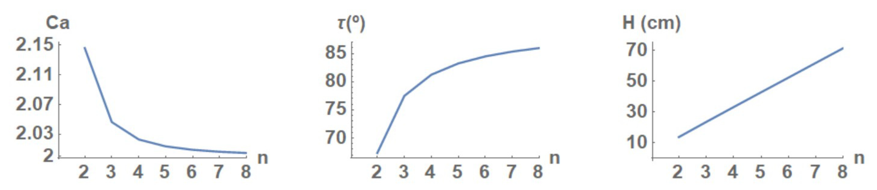
Case B	B1

shows the concentrations $C_{opt}$, optimal angles ${\tau }^{*}$ and heights corresponding to each $A_n$. Recall that as our method ensures that ${\eta }_{ray}=1$, we always have $C_{opt}=C_a$. The lack of influence of the longitudinal study implies that $B=b·C_a$.

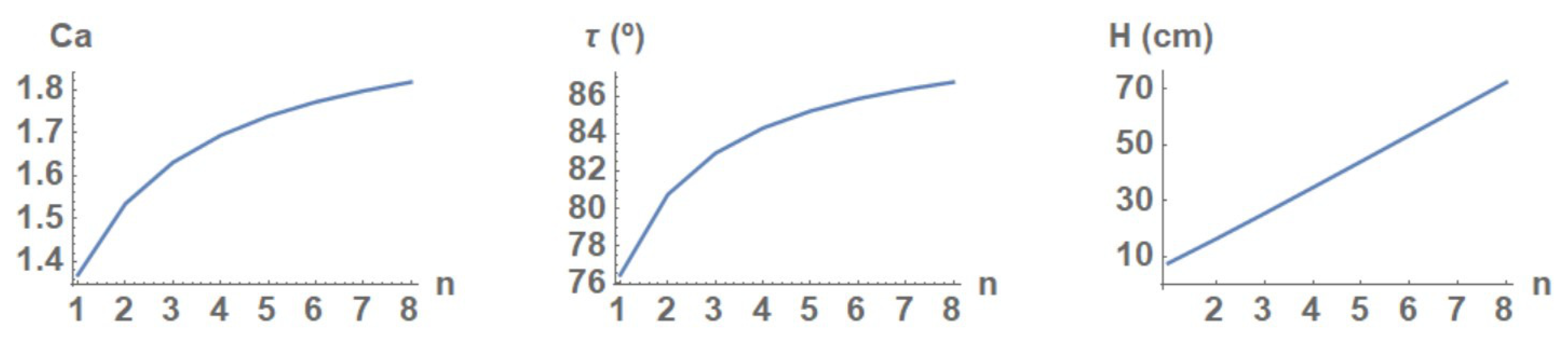
Figure 4 shows in a clearer way the evolution of the three parameters above. Notice how H is linear in n, but ${\tau }^{*}$ is (obviously) not, as it tends asymptotically to ${90}^{°}$.

The largest value of $C_{opt}$ (these are computed numerically) corresponds to the first physically possible case, $A_2$. The values decrease with n and approach the ideal value (2) asymptotically from above (in this specific example, ${sin}^{-1}{\theta }_C=2$). This phenomenon happens for any value of ${\theta }_c$ and is quite relevant, as it implies the number of reflections n is less (so that ${\rho }_m^n$ is greater) and also a lesser height H of the cavity (and, hence, less $R_a$).

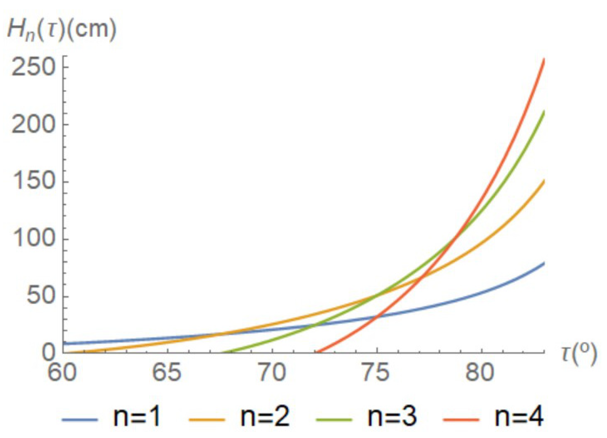
Finally, we need to check whether the solutions above are also valid for some case B. To this end, we use the family of curves $H_n\left(\tau \right)$ given by (29) (Figure 5 contains the first four of these). For a fixed b, this sequence of functions is valid for any value ${\theta }_c$, which simplifies the computations. Notice how as $\tau$ increases, the largest height (which is given by the envolvent of the curves) is reached for a greater number of reflections n. Even though the envolvent gives the maximum value of H, there may be cases $B_n$ with less n which also satisfy the condition (which is good, as it means a lesser number of reflections).

Thus, the last step of the optimization algorithm consists of taking the first optimal solution $A_n$ (for decreasing values of $C_{opt}$) which also satisfies the condition of case B. In this example, for $A_2$, we have ${\tau }^{*}=67.36$, $H=13.74$, and

$$H_1\left({\tau }^{*}\right)=16.87>H=13.74$$

(30)

So the best candidate $A_2$ is also valid because the conditions of case $B_1$ hold. However, this might not always be the case, as we will see later.

Ray Tracing Simulation and Verification

We verified our results using a Matlab™ray-tracing program which models solar power optical systems [37,38], using geometric optics. This program has already been used in other studies [38,39].

Figure 6 contains the simulation of our two-foci V-trough concentrator for ${\alpha }_0={30}^{°},{40}^{°}$ and ${50}^{°}$. Notice how for ${\theta }_i\le {\theta }_c$ (the incidence angle), all the rays reaching the base B end up on the cells at b, as shown in Figure 6a. For ${\theta }_i>{\theta }_c$, part of the rays entering the cavity end up at b (Figure 6b), and finally, the worst case happens for ${\theta }_i\gg {\theta }_c$, when no ray entering the cavity reaches b.

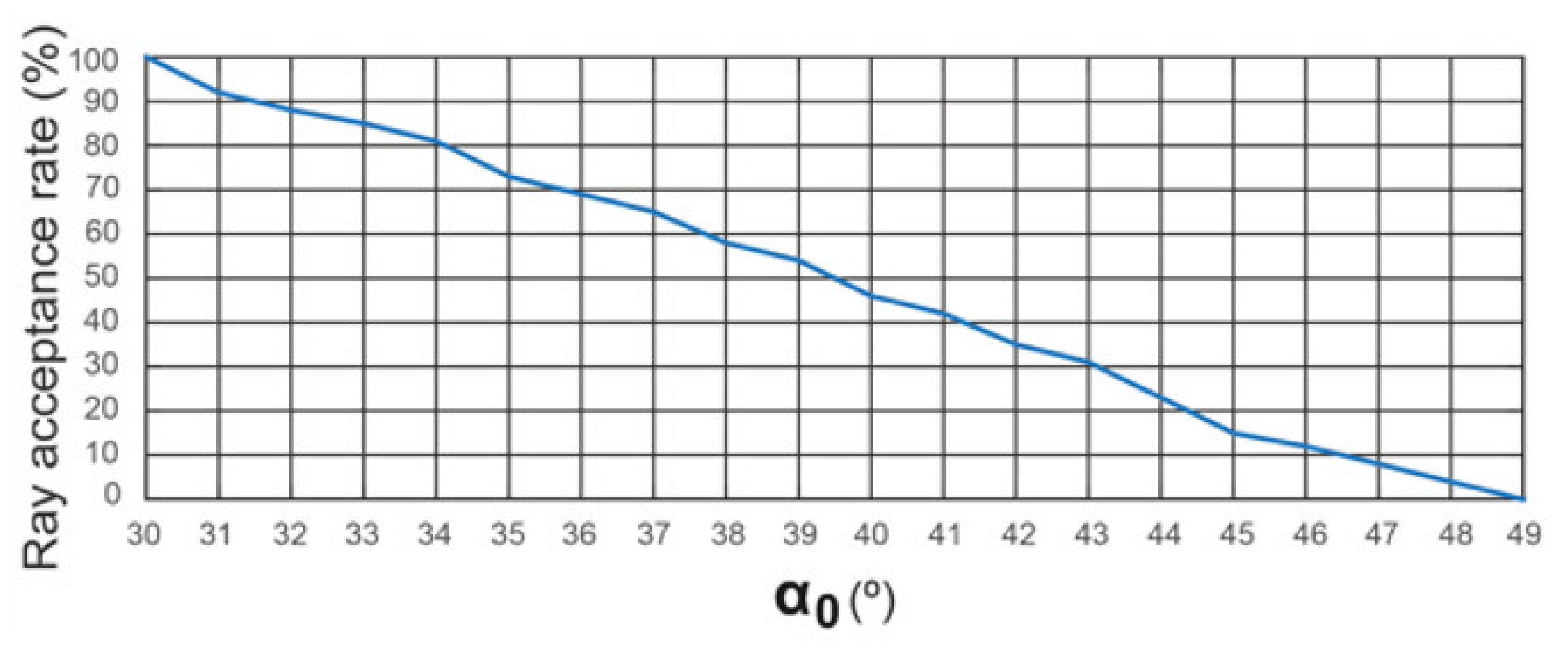
In Figure 7 we provide an analysis of the evolution of the ray acceptance rate ${\eta }_{ray}$ for angles ${\theta }_i$ greater than ${\theta }_c$. Recall that in ideal $CPCs$, this value goes from one to zero instantaneously [33]. In the classical V-trough [33], ${\eta }_{ray}$ decreases depending strongly on the incidence ray and the design of the cavity. One can see that in our model, one goes from ${\eta }_{ray}=1$ for ${\theta }_i\le {\theta }_c$ to decreasing values in a progressive but not too sharp a way. This is, in our opinion, another strength of our proposed design.

As a cost analysis, we compute the reflector-to-aperture area ration $R_a$, disregarding the length, which has no relevance:

$$\left.\begin{array}{c}{A}_r=2{\displaystyle \frac{H}{sin{\tau }^{*}}}=2.977\hfill \\ A_a=2.146\hfill \end{array}\right\}\to R_a=\frac{A_r}{A_a}=1.387$$

(31)

5. Comparison with Other Classical Receivers

Finally, we compare our design with two different classical concentrators: the classical V-trough and the ideal CPC. We do this for several acceptance angles ${\theta }_c$.

5.1. One-Focus V-Trough

For ease of comparison with the two-focus design proposed here, the classical one-focus V-trough design is shown. Using Property 1, we start the iterative algorithm stating a sequence of different cases $C_n$ for an increasing number of reflections n. We will use, in each of them, the worst-case condition ${\theta }_i={\theta }_c$. For each case $C_n$, the height of the cavity $H_n$ can now be computed using (12), (13) and (21):

$$H_n\left(B\right)={\sum }_{i=1}^n{l}_i$$

(32)

Now, we substitute the value of $H_n\left(B\right)$ into the formula relating $b,B$ and H with $\tau$:

$$B=b+2H_n\left(B\right)cot\tau$$

(33)

and, solving for B, after some easy computations, we obtain:

$$\begin{array}{cc}\hfill C_1& :B_1\left(\tau \right)=-bcos({\alpha }_0-3\tau )sec({\alpha }_0-\tau )\hfill \\ \hfill C_2& :B_2\left(\tau \right)=bcos({\alpha }_0-5\tau )sec({\alpha }_0-\tau )\hfill \\ \hfill C_3& :B_3\left(\tau \right)=-bcos({\alpha }_0-7\tau )sec({\alpha }_0-\tau )\hfill \\ \hfill & \cdots \hfill \\ \hfill C_n& :B_n\left(\tau \right)={(-1)}^{n}bcos({\alpha }_0-(2n+1)\tau )sec({\alpha }_0-\tau )\hfill \end{array}$$

(34)

This gives the functions $B_n\left(\tau \right)$ analytically in terms of b and ${\alpha }_0$. In the last step of the algorithm, we need to compute the maximum of those $B_n\left(\tau \right)$ in order to obtain the optimum angles ${\tau }_n^{*}$ maximizing B and hence $C_a$.

The process can be made as long as desired, and we can choose the optimal design depending on the number of reflections n. From the qualitative point of view, the main result is that the larger n, the larger $B_n$, so that $C_a$ increases as well. Actually, $C_a$ tends asymptotically to the ideal value (2). In each case $C_n$, the number of reflections is n.

Recall that our design guarantees ${\eta }_{ray}=1$.

Table 2. Example of optimal design of a V-trough.

Case C	C1	C2	C3	C4	C5	C6	C7	C8
$C_{opt}$	1.369	1.535	1.631	1.694	1.738	1.772	1.797	1.818
${\tau }^{*}$${(}^{°})$	76.44	80.75	82.96	84.31	85.22	85.88	86.38	86.77
H (cm)	7.66	16.43	25.55	34.83	44.18	53.59	63.03	72.49

and Figure 8 summarize our results for $b=10$ and ${\theta }_c={30}^{°}$.

Notice how $C_n$ approaches the ideal value $C_{opt}={sin}^{-1}{\theta }_C=2$ but forcing the walls to become practically vertical ($\tau \to {90}^{°},\mathsf{\Phi }\to 0^{°}$). This follows easily from (5) (see [35]):

$$C_a=\frac{1}{sin({\theta }_C+\mathsf{\Phi })}$$

(35)

Quoting [35], “We see that a V-trough can, at least in principle, approach the ideal concentration if it is very narrow, that is if $\mathsf{\Phi }\to 0^{°}$. In that limit, however, the number of reflections as well as the aperture to reflector ratio become very unfavorable”. Furthermore, as n increases, H does so much faster, and the factor ${\rho }_m^n$ decreases the power reaching the PV cells.

Table 3. Comparative table for several ${\theta }_c$.

${10}^{°}$	V-2F	CPC	V-1F	${30}^{°}$	V-2F	CPC	V-1F
Case	A5-B4		C6	Case	A2-B1		C2
$C_{opt}$	5.829	5.759	3.733	$C_{opt}$	2.146	2.000	1.535
$\tau$	80.99		85.09	$\tau$	67.36		80.75
H	152.5	191.6	158.9	H	13.74	25.98	16.43
n	0.977	1.043	0.989	n	0.468	0.674	0.522
$R_a$	5.295	6.774	8.55	$R_a$	1.387	2.674	2.169
${15}^{°}$	V-2F	CPC	V-1F	${35}^{°}$	V-2F	CPC	V-1F
Case	A4-B2		C4	Case	A2-B1		C2
$C_{opt}$	3.934	3.864	2.616	$C_{opt}$	1.849	1.743	1.418
$\tau$	79.06		83.41	$\tau$	69.27		81.37
H	75.89	90.76	69.95	H	11.22	19.59	13.78
n	0.847	0.902	0.822	n	0.439	0.621	0.502
$R_a$	3.930	4.813	5.38	$R_a$	1.298	2.308	1.966
${20}^{°}$	V-2F	CPC	V-1F	${40}^{°}$	V-2F	CPC	V-1F
Case	A3-B2		C3	Case	A2-B1		C2
$C_{opt}$	3.017	2.924	2.067	$C_{opt}$	1.633	1.555	1.325
$\tau$	75.40		82.16	$\tau$	71.17		82.04
H	38.73	53.90	38.76	H	9.28	15.23	11.63
n	0.701	0.807	0.701	n	0.411	0.572	0.480
$R_a$	2.653	3.792	3.786	$R_a$	1.201	2.006	1.773
${25}^{°}$	V-2F	CPC	V-1F	${45}^{°}$	V-2F	CPC	V-1F
Case	A3-B1		C3	Case	A2-B1		C2
$C_{opt}$	2.431	2.366	1.817	$C_{opt}$	1.471	1.414	1.250
$\tau$	76.44		82.52	$\tau$	73.06		82.76
H	29.68	36.09	31.12	H	7.73	12.07	9.84
n	0.669	0.734	0.684	n	0.382	0.525	0.456
$R_a$	2.512	3.141	3.455	$R_a$	1.099	1.743	1.587

contains the summary of this study for ${\theta }_c\in [10,45]$ in steps of $5^{°}$.

5.2. CPC

The design of a CPC is basically a pair of skewed parabolas whose length is such that at the extremes the parabolic arcs are parallel to the axis of the concentrator. The angle between the axis of the CPC and the line connecting the focus of one of the parabolas with the opposite edge of the aperture is the acceptance half-angle ${\theta }_c$. When the reflector is ideal, any radiation entering the aperture at angles between $\pm {\theta }_c$ will be reflected to the base of the concentrator. However, CPCs must be very high to achieve great concentrations, and they are usually truncated in order to cut them down from h to an acceptable height $h_T$. This truncation is convenient for the reflector-to-area ratio, and the decrease in performance (acceptance angle and concentration ratio) is low. See Appendix A for the relevant formulas.

5.3. Results

Table 3 contains the comparison for ${\theta }_c\in [10,45]$ (°) between our design and the other two concentrators. We provide the values of three parameters: optical concentration ratio $C_{opt}$, optimum angle ${\tau }^{*}$ and height H, and the cost parameter $R_a$. We also show the combinations of cases A and B yielding our optimal design. The values for the CPC correspond to the ideal case (in the formulas of the Appendix A, ${\varphi }_T=2{\theta }_C$, $a_T=a$, and $h_T=h$). To compute the average number of reflections n, we used the formulas for the truncated CPC with the same height as our two-foci V-trough. In order to give a meaningful comparison with the classical V-trough, we have chosen the case $C_n$ with the same height as our design.

We remark the following:

• Our solution is clearly better than the classical one-focus V-trough in optical concentration ratio $C_{opt}$, with an increase between $15.02$ and $35.95\%$. It is also better from a cost-analysis point of view, as our $R_a$ is generally $46.63\%$ better.
• As regards the CPC, our $C_{opt}$ is always slightly better (around $4\%$). The height H is notably less in our design (around $54.33\%$), which leads to a much more compact element, and $R_a$ is generally $57.63\%$ less. Notice that our design is much easier to build than the CPC, obviously.

6. Conclusions

The design of the secondary cavity of a small-scale linear Fresnel reflector is key to maximizing the concentration ratio, which allows for a decrease in the number of photovoltaic cells required and for an increase in the width of the mirrors of the primary field, both of which lower the final cost.

In this work, we have computed analytically, the optimal design of a cavity which, using a non-symmetric distribution of the irradiance reaching its opening, has a concentration ratio greater than those of classical designs. Our analytic approach provides formulas for any number of reflections, which are easily implemented as an iterative algorithm. Furthermore, we prevent the combinatorial explosion inherent in ray-tracing.

We use a two-foci configuration in which rays from each side of the small-scale linear Fresnel reflector reach the other side of the secondary cavity, so that the distribution of irradiance cannot be assumed uniform. We show that our design produces an optical concentration above the ideal value for classical concentrators with uniform distributions. The values for the reflector-to-aperture area ratio are also better, and the design is both more compact and easier to build. Finally, our proposal always yields a value of ${\eta }_{ray}=1$, as the classical compound parabolic concentrator, but for ${\theta }_i>{\theta }_c$, the values of ${\eta }_{ray}$ decrease progressively but slowly.

Future research might include the possibility of modifying the design to have two secondary cavities instead of just one, one on each side of the small-scale linear Fresnel reflector. This would halve the acceptance ratio while notably increasing the concentration. However, there would probably be a cost increment which should be taken into account. This study can be applied to daylighting systems using fibre optics.