Article

Computational Analysis of Tube Wall Temperature of Superheater in 1000 MW Ultra-Supercritical Boiler Based on the Inlet Thermal Deviation

1
Institute of Thermal Science and Power Systems, Zhejiang University, Hangzhou 310027, China
2
Zhejiang Provincial Key Laboratory of Energy Conservation & Pollutant Control Technology for Thermal Power, Zhejiang Zheneng Technology Research Institute Co., Ltd., Hangzhou 311121, China
3
Zhejiang Province Energy Group Co., Ltd., Hangzhou 310007, China
4
State Key Laboratory of Clean Energy Utilization, Institute of Thermal Power Engineering, Zhejiang University, Hangzhou 310027, China
5
Zhejiang Zheneng Zhongmei Zhoushan Coal & Electricity Co., Ltd., Zhoushan 316131, China
*
Author to whom correspondence should be addressed.
Energies 2023, 16(3), 1539; https://doi.org/10.3390/en16031539
Submission received: 12 January 2023 / Revised: 30 January 2023 / Accepted: 1 February 2023 / Published: 3 February 2023

Abstract

:
Local over-temperature is one of the main reasons for boiler tube failures (BTF). By accurately monitoring and controlling tube wall temperature, local over-temperature can be avoided. Based on the measured flue gas parameters and numerical simulation, a method of thermal deviation calculation is proposed in this study for the on-line calculation of the tube wall temperature of boiler superheaters. The full-size three-dimensional numerical simulation was presented on the combustion in a pulverized coal-fired boiler of 1000 MW ultra-supercritical (USC) unit. A difference in the thermal deviation of the vertical direction was innovatively introduced into a segmented discrete model, and the thermal deviation condition conforming to reality was introduced into the calculation. An on-line calculation system developed based on the current calculation method was applied in a 1000 MW USC unit. The calculated local high-temperature zone was consistent with the actual over-temperature position and conformed to the law of the allowable metal temperature of the final superheater (FSH) serpentines segment. The comparison results showed that the calculated data by this method were more reflective of tube wall temperature change with boiler loads than the measured data. According to the calculated local over-temperature zone, the immediate warning response can effectively reduce the possibility of over-temperature BTF.

1. Introduction

Even with new and clean energy technologies developing rapidly in recent years, coal-fired power generation is still the main source of electric power [1]. By the first quarter of 2022, coal-fired power generation accounted for 46.1% of the total installed capacity in China [2]. Due to their higher efficiency and less harmful emissions compared with traditional coal-fired power generation, ultra-supercritical (USC) units have become increasingly popular in the coal-fired power industry, especially for 1000 MW USC units with ultra-low emissions, deep peak regulation and other technologies. By the first quarter of 2022, 75 1000 MW USC units had been under operation in China, and another 10 units were under construction. In a 1000 MW USC unit, the width of the boiler is generally more than 30 m. Its large span leads to combustion inhomogeneities along the width of the boiler. Thus, both the temperature and velocity distributions of flue gas show large deviations along the horizontal direction [3]. According to measured data, the thermal load deviation of the superheater and reheater are between 1.15 and 1.25 [4]. The large deviation may result in the locally excessive temperature being higher than the allowable temperature of the metal material. Long service under over-temperature conditions causes the exfoliation of steam-side oxide scales, reducing the stress rupture life, and even overheating and boiler tube failures (BTF) [5]. About 40% of the emergency shutdowns of units are caused by BTF [6], which is a loss of approximately USD 5 billion per year for the power industry [7].
Adjusting the boiler combustion operation is the most rapid, convenient and efficient way to solve the problem of local over-temperatures on high-temperature heating surfaces. However, the problem usually occurs in the area with high temperature and high ash, so the exact locations of over-temperature local areas are difficult to obtain in real-time during the daily operation of the boiler. Many temperature measurement points are arranged in the USC units to detect over-temperature circumstances during the daily operation of the boiler. Considering the service life, the measurement points are not arranged on the high-temperature heating surfaces inside the boiler, but on the wall of serpentine outlet steam pipes outside the boiler. Combined with the calculation based on the flow and heat transfer mechanism model of flue gas and working fluid, the over-temperature circumstance of a whole tube can be well understood. However, the results mainly reflect the overall over-temperature of the serpentines. For the situation where the overall heating surface tube is not overheated, while the local tube segments are overheated, effective information obtained from the measured temperature data is limited. Thus, the combustion operation cannot be adjusted in a timely manner, according to the real-time situation, and eliminate persistent over-temperature of local areas. Finding a means to obtain accurate temperatures of the high-temperature heating surface in real-time is the key to solve the problem of over-temperature BTFs.
Many studies use theoretical calculation methods to obtain the real temperature on high-temperature heating surfaces that are mainly based on the method described in the Thermal Calculations of Steam Boilers [8] and ASME IAPWS-IF97 [9]. Based on the premise of the mass and energy balance, considering the inhomogeneity of heat absorption along the cross section and perimeter of the pipe, the thermal characteristic along the tube wall, hydraulic inhomogeneity, and structural differences in the serpentine pipe, the tube wall temperature can be calculated. In recent years, many improvements have been proposed. Wang et al. [10,11] introduced the thermal deviation theory of the same platen and the same piece to distinguish the difference and the flow deviation between different serpentine tubes in the same tube platen. Xu et al. [4] proposed a thermal load model based on the power plant thermodynamic parameters, thermal deviation theory, and flow rate deviation theory. The BTF positions predicted by this model are the same as those in the reheater of a 300 MW utility boiler. Prieto et al. [12] described a three-dimensional numerical model, and the continuity, momentum, and energy equations were solved in a coupled way, calculating the temperature of the tube surfaces along the reheater. Madejski et al. [13] presented a model based on the combination of the CVFEM and finite difference method. The steam and tube wall temperature were computed in the superheater using this model and compared with the results obtained by CFD simulation. Taler et al. [14,15] used a finite difference model with distributed parameters to solve energy conservation equations for steam, tube wall, and flue gas. Trojan et al. [16,17] developed distributed parameter mathematical models of the steam superheater’s individual stages. Using the iterative calculations of the steam, flue gas, and air temperatures, the developed mathematical models make it possible to determine temperatures of the tube outer and inner surfaces. Xu et al. [18] proposed a single tube model based on the finite volume method and measured temperature. Considering the temperature distributions, both of the steam side and the flue gas side, the tube wall temperature with a variety of combinations, including different steam flow rates and heat transfer coefficients, were determined, and the tube wall temperature profiles of the superheater and reheater tubes in the power plant were evaluated. Based on thermal deviation theory and local energy and mass balance of the superheater tube, Sun et al. [19] proposed a method of calculating tube wall temperature, adding the thermodynamic constraint condition to the calculation of the steam temperature of the cross section. The calculated maximum wall temperature position coincided with the position of the actual overheating tube. In order to simplify the calculation model, many assumptions were made when calculating the temperature of the heated surface wall in the mentioned research; for example, circumferential heat conduction in the tube wall was assumed to be negligible, pressure along the steam flow was constant, the temperature and flue gas velocity were constant over the channel cross section before the superheater, and the load of the boiler was constant. The calculated results were too idealized to quickly and accurately obtain the heating surface wall temperature under varying boiler loads.
In addition to the above theoretical calculation methods, computational fluid dynamics (CFD) simulation is also used to evaluate the tube wall temperature [20,21,22]. The combustion process of the boiler and the heat transfer process of the high-temperature heating surface are always modeled in different computational domains. Heating surfaces are modeled as porous regions, while direct radiation is set as a complement of a heat source term. In this way, CFD simulation is useful for obtaining the temperature field and velocity field of flue gas of the heating surface, but not the tube wall temperature. Moreover, the operating state of a boiler in an actual power plant deviates greatly from design values or theoretical conditions. Especially for opposite firing boilers, the primary air flow (the air used for drying pulverized coal and carrying the dried pulverized coal into the furnace) and fuel flow are different between different burners, and the secondary air flow (the air enters the furnace directly through the secondary bellow after being heated by the air preheater) in the air box has different distribution characteristics due to the violent combustion in the furnace [23]. The calculated temperature field and velocity field model show the characteristics of left–right symmetry because of the boundary condition settings for different burners in a fully symmetrical and equal way, which are far from actual conditions.
In order to obtain accurate tube wall temperature distribution and the local over-temperature zone of FSH in a 1000 MW opposite firing boiler during actual operation, operators must adjust the operation parameters in time to avoid the local over-temperature state of the heating surface for long periods of time. In this study, by measuring the excess air coefficient at the inlet of the air preheater under hot operation of the boiler, the horizontal air distribution coefficient of the boiler was obtained. The secondary air flow of different burners was determined according to the actual opening of the secondary air baffle of the burners. The horizontal air distribution coefficient and secondary air flow were set as the input boundary conditions. Via the full-size numerical simulation for a boiler, the flue gas temperature distribution at the inlet cross section of the FSH was obtained, and it was further amended by arranging gas temperature measuring results at the same cross section. The amended temperature distribution was then set as the thermal deviation condition for the calculation of tube wall temperature of the FSH. With the segmented finite element method, the tube wall temperature distribution on the FSH of the boiler under different loads was obtained. Compared with previous methods, the method reported in this study is a better fit with the actual operation of the boiler, and more accurately reflects the local over-temperature of the FSH. Due to its good performance in over-temperature warning, the on-line calculation system of wall temperature based on the new method has been successfully applied to an opposite firing boiler in a 1000 MW USC unit. It has been verified that the calculated results are more consistent with the local temperature change than the data obtained from measured points.

2. Case Study Boiler

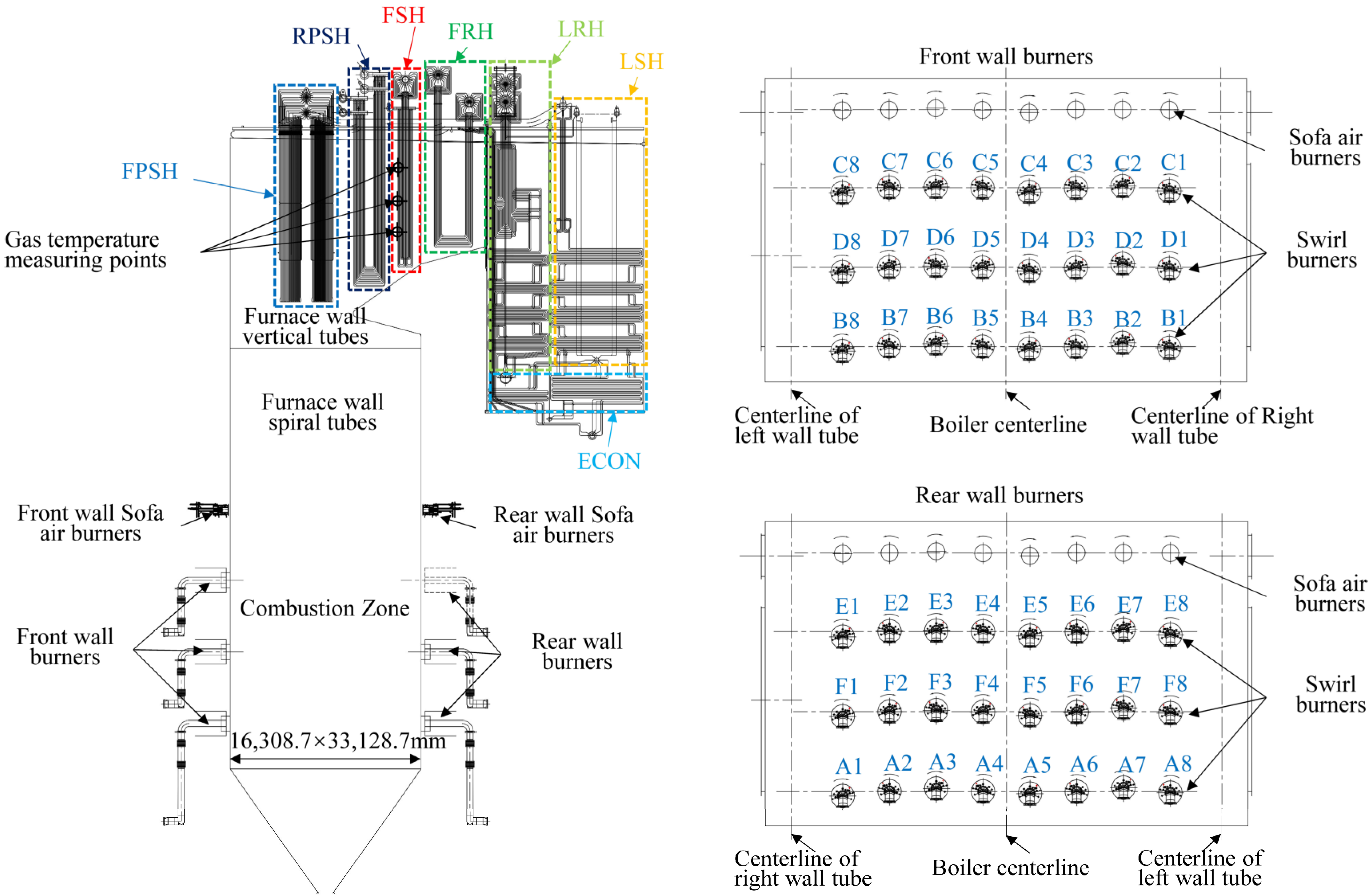
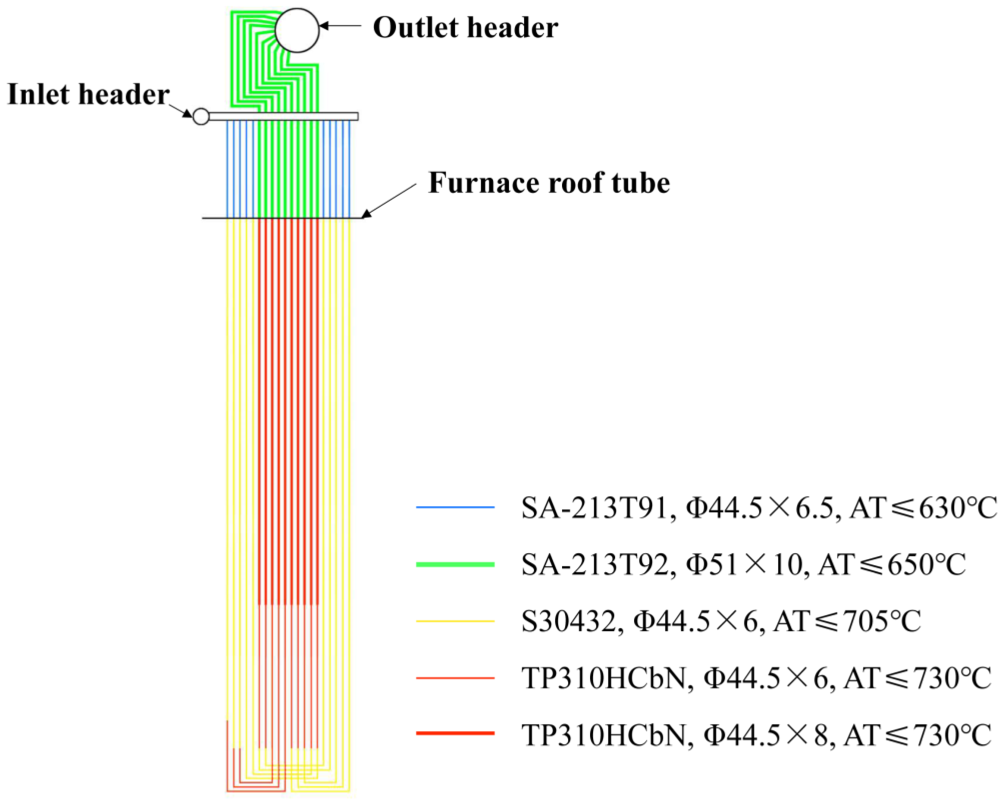
2.1. Opposed Firing Utility Boiler Specifications

The numerical simulations were performed for a π type pulverized coal-fired boiler in a 1000 MW USC unit. The layout of burners and high-temperature heating surfaces of the boiler are shown in Figure 1. The length, width, and height of the furnace were 16,308.7 mm, 33,128.7 mm and 64,500 mm, respectively. There were 48 swirling burners arranged in an opposed firing way on the front and rear walls. The 24 swirling burners on each wall were averagely divided into three layers. Burners in the same layers were staggered in the vertical direction, and the swirl directions of any two adjacent burners were the opposite. Along the flue gas flow, the front platen superheater (FPSH), rear platen superheater (RPSH), final superheater (FSH), final reheater (FRH), low temperature reheater (LRH), low temperature superheater (LSH), and economizer (ECON) were heated successively. The FSH consisted of 110 tube platens along the width direction of the furnace, with a transverse intercept of 300 mm. From right to left were tube platen 1 to tube platen 110 in sequence. For each tube platen of the FSH, as shown in Figure 2, the serpentine was arranged with five kinds of steel tubes. According to the thickness and the allowable temperature (AT) of the material for each steel tube, the thermostability of the three tube segments below the furnace roof tube increased gradually, from inlet header to outlet header.
A total of 21 S-type thermocouples were installed at the inlet of the FSH under the cold state of the boiler beforehand. These thermocouples were equably distributed on the three layers of the flue cross section (Figure 3). Signals from these thermocouples are introduced into the distributed control system (DCS) of the power plant to obtain the inlet gas temperature distribution of the FSH under the hot state of the boiler. The thermocouples were supposed to be unacted on the heat radiation from burning, because the thermocouples were installed above the furnace arch and used RPSH as a shield. Since the thermocouples were installed at the same cross section, the radiation on thermocouples from the furnace and the wall is mainly related to gas dimensionless coefficient numbers (e.g., Nusselt number and Reynolds number), gas temperature and blackness, tube wall temperature, and the Boltzmann constant [24]. These parameters are approximately equal under the same load and the same flue surface; thus, they have limited influence on the relative value of flue gas temperature between different measuring points. The mass flow rate of flue gas under the rated load was Qs = 3568 t/h, the density was ρg = 1.323 kg/Nm3, and the inlet temperature was Tg,in = 990 °C; the width of the flue cross section was W = 33,128.7 mm, the height was H = 12,784 mm, the pressure was Pg,in ≈ −100 Pa, and the velocity of flue gas was Vg,in ≈ 8.19146 m/s, calculated according to the following Equation (1). At low gas flow rate, the accuracy of the thermocouple measurement results can be guaranteed.
V g , in = Q s ρ g   ×   273 273 + T g , in   ×   101 , 325     P g , in 101 , 325   ×   W   ×   H

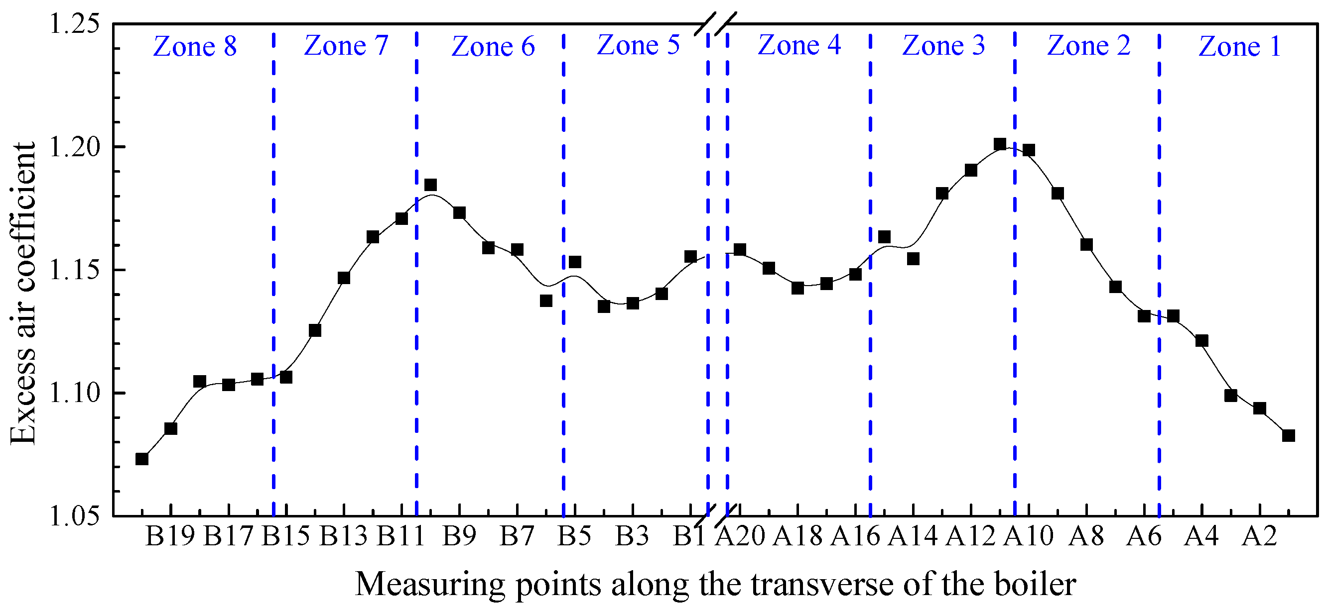
2.2. Measurement of Transverse Distribution of Excess Air Coefficient of Boiler

As described in the previous section, during hot operation of the boiler, intense combustion occurs in the center of the furnace, which consumes a large amount of air and makes an under-pressure environment in the central area of the furnace, resulting in a difference of under-pressure levels on the horizontal section of the furnace. For a 1000 MW opposed firing boiler with large air boxes on both sides, the secondary air (including SOFA air) flow of each burner is different under the same secondary air baffle opening; specifically, the secondary air flow in the middle of the furnace is relatively large, and the secondary air flow on both sides is relatively small. Two factors are related to this phenomenon; one is the horizontal width of the boiler, the other is the differential pressure between static wind boxes (about 0.3 and 0.5 kPa) and the furnace. Due to the horizontal width of the boiler being more than 30 m and with eight installed burners, the difference of under-pressure levels caused by intense combustion in the furnace tends to cause different secondary air flows in burners. As the pressure of primary air is as high as 1.2 kPa, flow imbalance is not obvious for the primary air.
Due to the burner structure, it is very difficult to measure the difference in secondary air flow of different burners in the hot state of a boiler, and it is impossible to simulate the combustion pressure in the cold state. According to the method described by Zhou [23], 40 measuring points were set horizontally in the outlet section of the economizer at the end of the boiler. After 5 h of stable running of the boiler, the average excess air coefficient of the 40 points was measured. The section was divided into eight regions. Since the horizontal flow rate of the flue gas is much lower than the vertical flow rate in the furnace [25,26], the difference in excess air coefficient in the eight regions can be considered as the difference in secondary air volume of the burner. Thus, the deviation coefficient of secondary air volume of the eight burners on the same layer of the burner can be settled.

3. Mathematical Model and Calculation Method

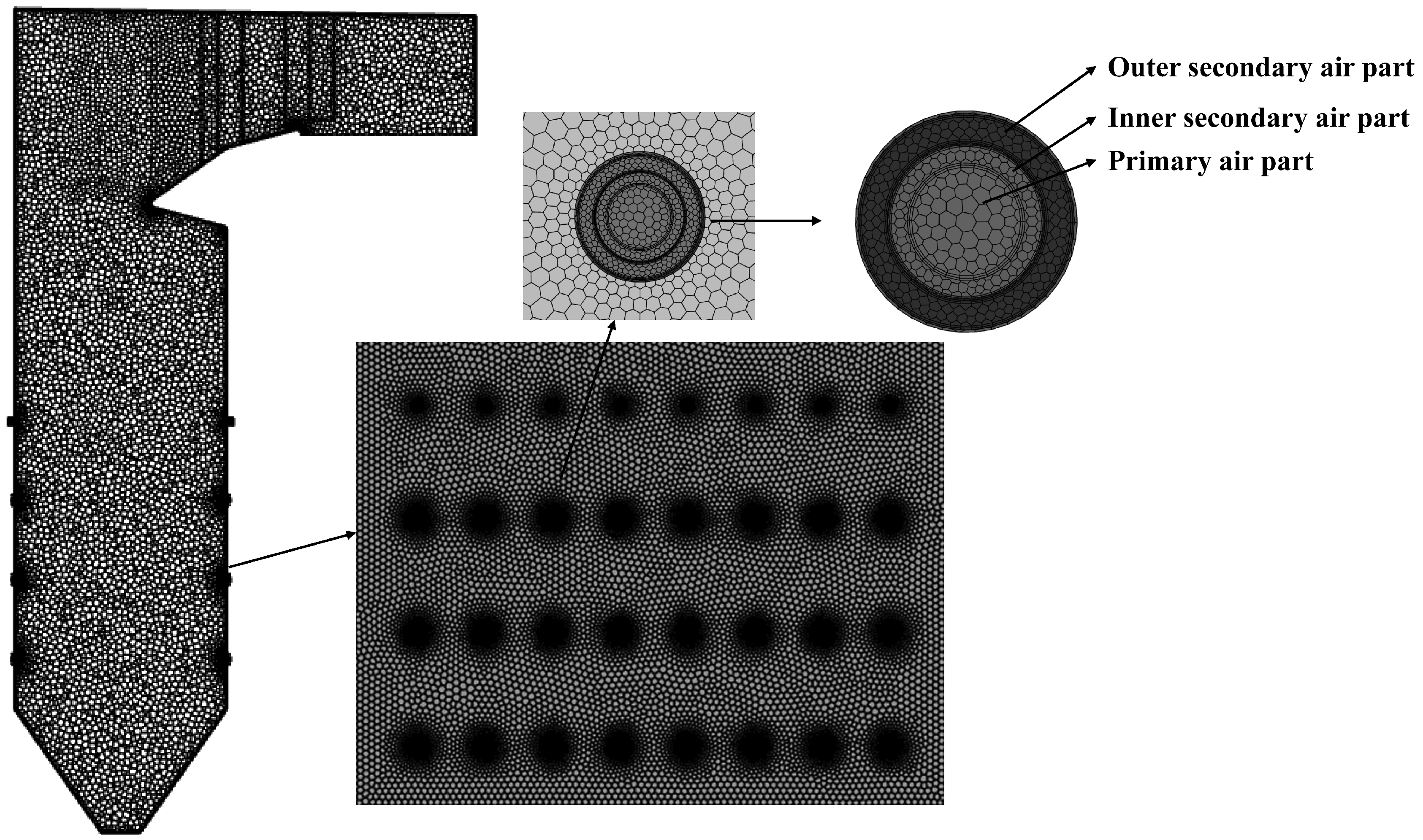
3.1. Mesh System and Boundary Conditions

A full-size calculation was employed in the model. The computational domain ranged from dry bottom hopper to horizontal flue outlets, including a furnace, DRB-4ZTM swirling burners, SOFA air burners, a superheater, and a reheater of the horizontal flue. After the verification of mesh independence, a polyhedral structure mesh comprising 1,767,143 polyhedral cells was established with Gambit, under the consideration of computational accuracy and workload, to simulate the combustion process of pulverized coal in the furnace (in Figure 4). To determine the main parameters of the boundary condition of the CFD model, measurements were taken from the DCS for a 5-h period, during which the unit load was kept stable at 100 and 75% rated load (most common loads of this unit). More details about the parameters are shown in Table 1. The primary air flow rate of eight burners on the same layer was set equally according to the total primary air flow rate of each coal mill. The secondary air flow rate of each burner under ideal conditions was obtained from the total secondary air flow rate, according to the relationship between the opening of the secondary air baffle and the secondary air flow rate, and then the actual flow deviation of the secondary air of each burner could be set according to the above-mentioned deviation coefficient of the secondary air flow of the burners.

3.2. Coal Combustion and Heat Transfer Models

Fluent 15.0 software was used to simulate the temperature of the pulverized coal combustion, gas flow, and heat exchange between heating surfaces. Combustion and heat transfer in the furnace is a complex physical and chemical process. It is necessary to select an appropriate mathematical model and parameters to obtain accurate results. A realizable k-epsilon model modified by rotational flow was employed in modeling gas flow. The Lagrange stochastic particle model was employed in modeling particle movement of pulverized coal. The eddy dissipation model was employed in modeling gas burning. The DO model was employed in modeling radiative transfer. The two-competing-rates model was employed in the devolatilization model. The diffusion dynamic model was employed in modeling coke combustion. The design parameters of the boiler under BMCR conditions were taken as boundary conditions for numerical simulation initially, in order to test the accuracy of the model by comparing the calculated flue gas temperatures on the same typical cross sections with the design data.

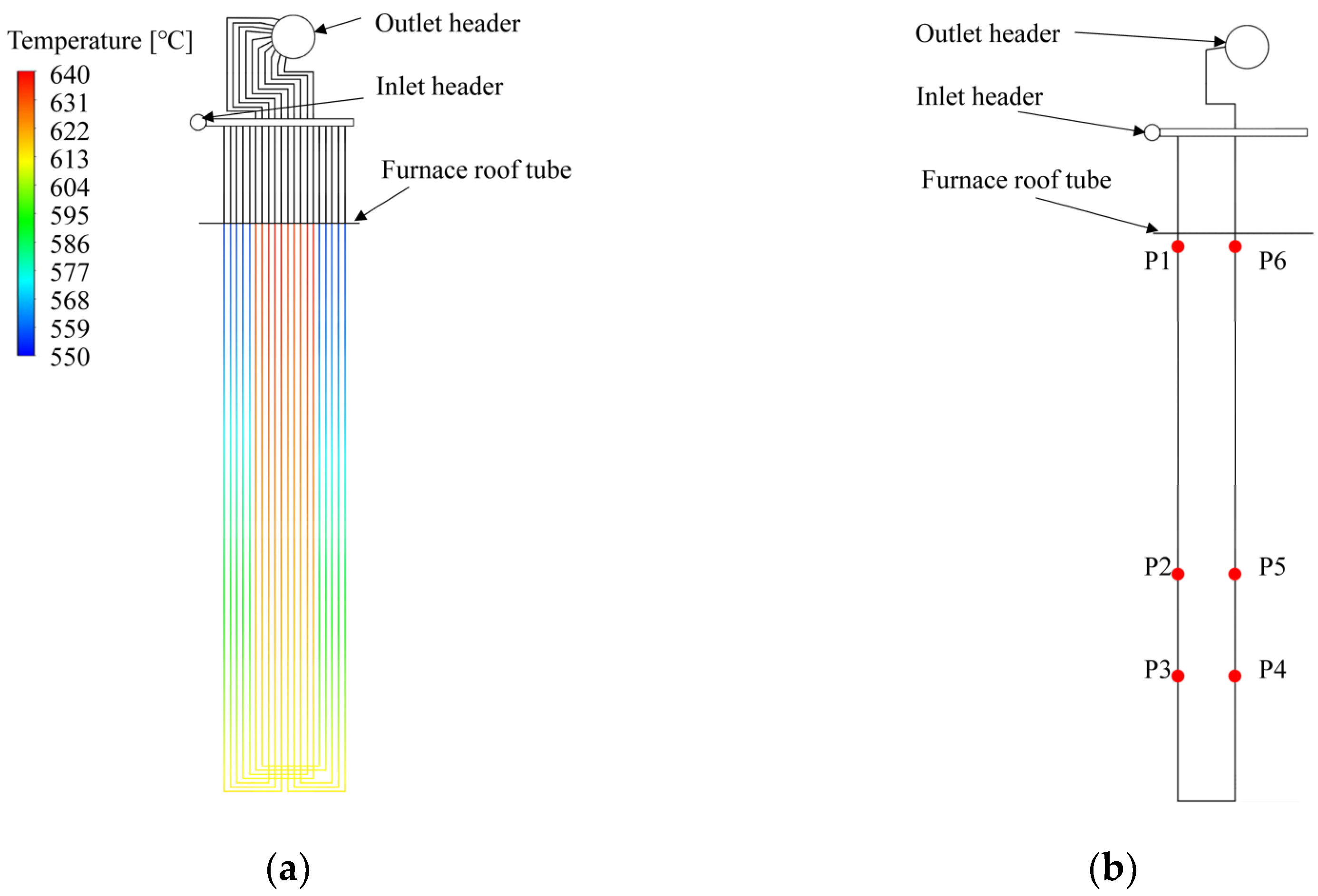
3.3. Method for On-Line Calculation of Tube Wall Temperature

Reference [27] described the on-line calculation method of tube wall temperature of a high-temperature heating surface based on the sliced and segmented model in detail. Firstly, the flue gas area of the whole superheater was dispersed into A × B × C heat transfer spaces through three-dimensional slicing and segmenting, in a direction perpendicular to the height of the furnace, in a direction perpendicular to the flue gas flow direction, and along the flue gas flow direction. Secondly, the serpentines were divided into several tube sections along the flow direction of the working fluid. Thirdly, based on the continuity and energy balance of gas flow and working fluid flow, the heat transfer quantity was determined. Fourthly, the tube wall temperature was calculated by the three-dimensional discrete model, by setting the thermal deviation condition and the hydraulic deviation condition satisfying the node mass flow continuity equation and the loop energy conservation equation. The similar method was also described in [14], the thermal deviation condition was estimated based on the tube wall temperature measured by thermocouples installed on the outlet of serpentines, reflecting the overall temperature condition of the serpentine. Obviously, the outlet tube wall temperature was not equal to the flue gas temperature and can only be divided by along the width of the boiler.
The calculation method for the thermal deviation coefficient was improved in this study. The real-time operation data and the measured excess air co-efficient deviation were used to conduct CFD full-size simulation. The calculation conditions were more consistent with the actual operation states of the boiler, so that the temperature distribution of the inlet section of the FSH calculated by numerical simulation was very consistent with the measured value. According to the flue gas temperature distribution at the inlet of the FSH, the thermal deviation co-efficient was divided in more detail along the width and height direction of the boiler, which previous researchers only considered the difference from the width direction. According to the different metal materials characteristics of different tube sections as shown in Figure 2, different thermal conductivity was used for different tube sections in the tube wall temperature on-line calculation. It should be noted that the tube wall temperature calculated by this method is not the highest temperature, but the arithmetic mean value of the inner and outer wall temperatures. The maximum tube wall temperature was located on the outer wall surface, which was about 10 °C higher than the arithmetic mean value of the inner and outer wall temperatures.

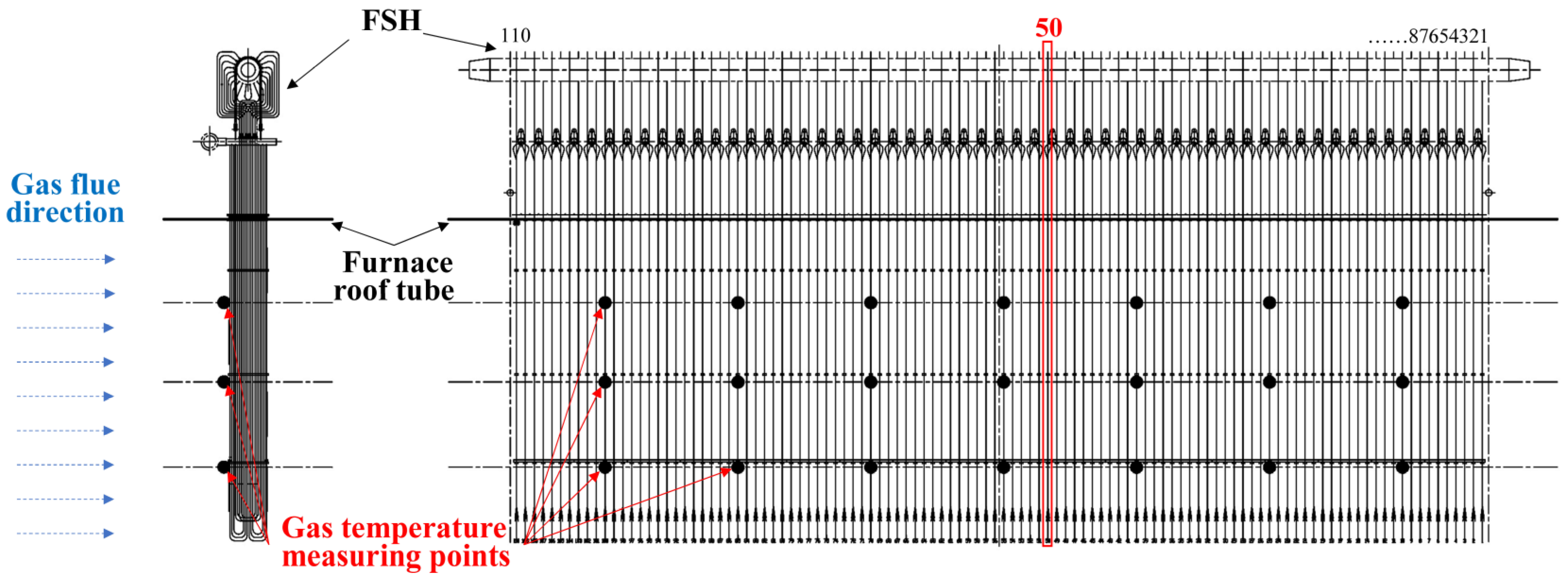
3.4. Thermal Deviation Model at the Inlet of the FSH

Relevant scholars [4,28,29] usually only paid attention to the transverse distribution of thermal deviation of the whole heating surface when calculating the tube wall temperature of the high-temperature heating surface. However, according to the flue gas temperature distribution of the FSH inlet section obtained in this study, there were obvious temperature differences in the vertical direction of the section. Only thermal deviation in the horizontal direction obviously brought great error to the subsequent tube wall temperature calculation. In this study, the inlet section of the FSH was divided into five regions in the vertical direction, and the thermal deviation of each region was calculated separately. By extension, thermal deviations under different loads and working conditions were obtained. Compared with previous studies which only took the transverse distribution of thermal deviation into account, the calculation of tube wall temperature in this study was much more accurate.

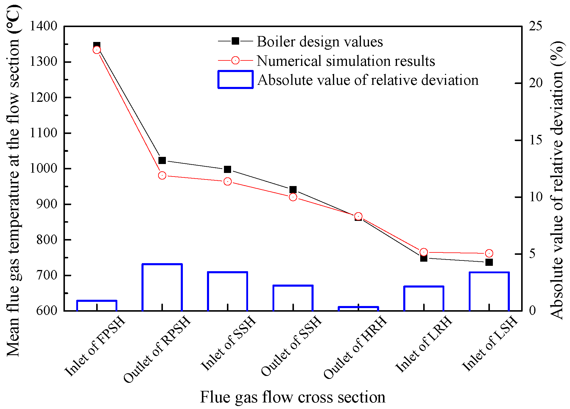
4. Results and Discussion

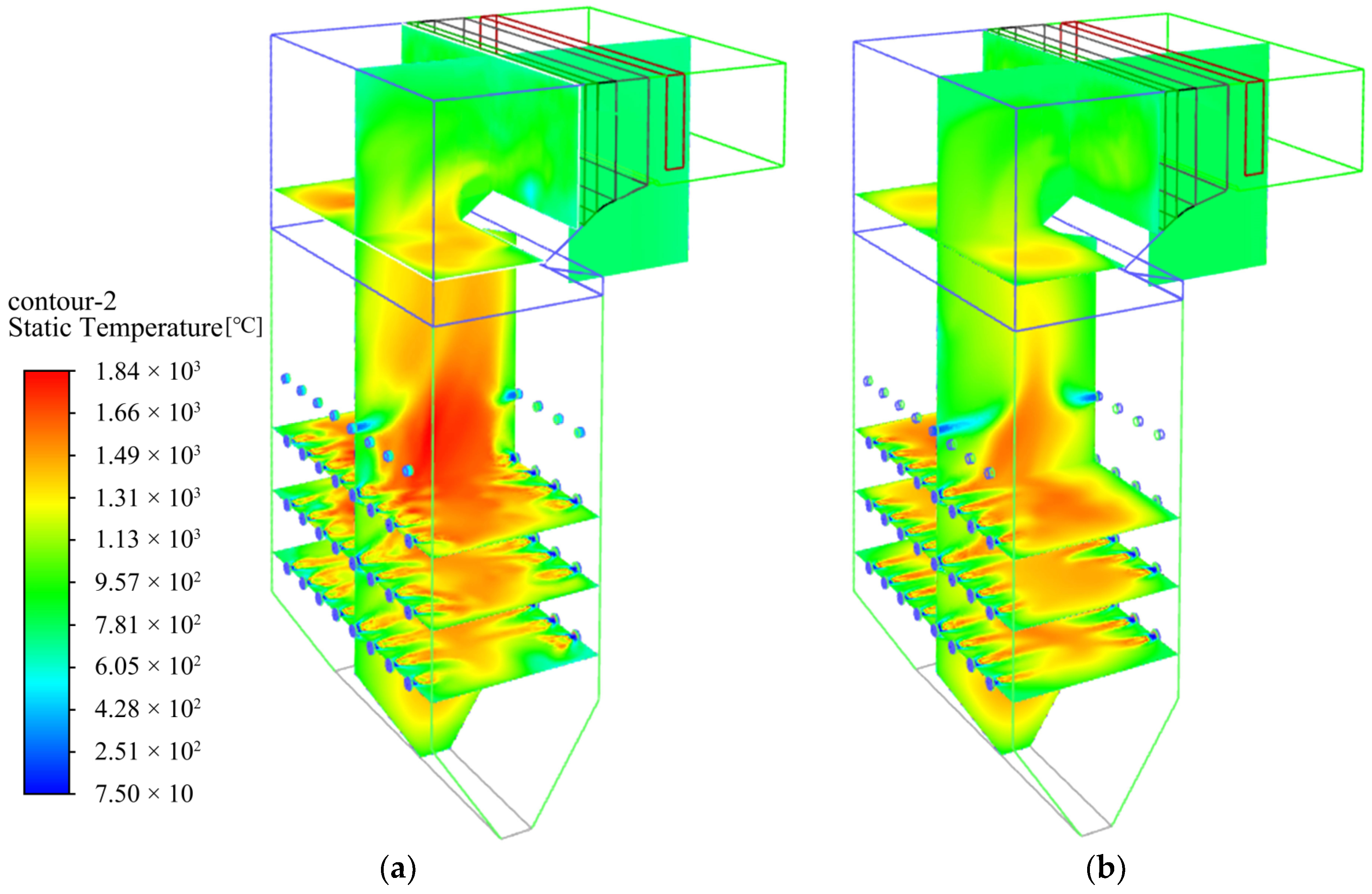
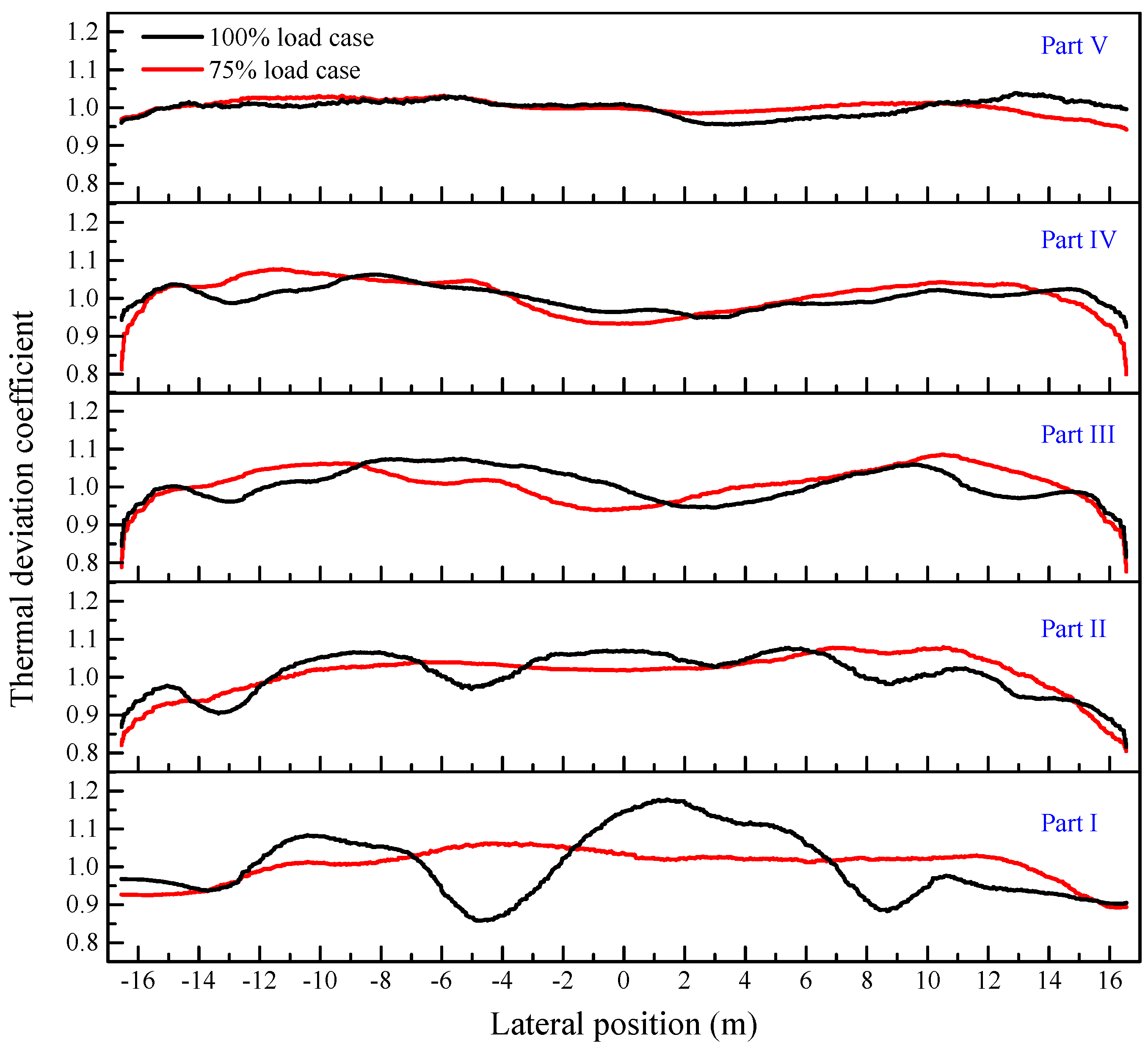
4.1. Distribution of the Thermal Deviation

The simulated flue gas temperatures at the inlet and outlet sections of the main heating surfaces under BMCR conditions are shown in Figure 5. All of the relative deviations between the calculated values and designed values were less than 5%. It indicates that the chosen models and the parameters setting were appropriate. Based on the excess air coefficient distribution along the width direction of the burner (Figure 6), the full-size three-dimensional numerical simulation was conducted for the temperature distribution in the furnace under the conditions of a 100% load case and a 75% load case. The simulated temperature distribution in the furnace is shown in Figure 7. The results show that the calculated flue gas temperature distribution (Figure 8a,b) at the inlet section of the FSH is very similar to the measured flue gas temperature distribution (Figure 8c,d). It can be seen that the numerical simulation results have a strong similarity with the measured results. The locations of the local high-temperature zone and local low-temperature zone obtained by the two methods were in good agreement. The insufficient number of measuring points led to the low accuracy of the measured temperature distribution; thus, the numerical simulation results differed slightly from the measured results. The results of the numerical simulation for the 100% load case and 75% load case show that the thermal deviation coefficient distribution changed significantly along the vertical direction. Figure 9 shows the distribution of the thermal deviation coefficient of the five vertical zones. The different thermal deviation coefficients indicate the nonuniformity of the flue gas temperature distribution. The simulation results confirm the necessity of zone divisions to improve the accuracy of the tube wall temperature calculation.

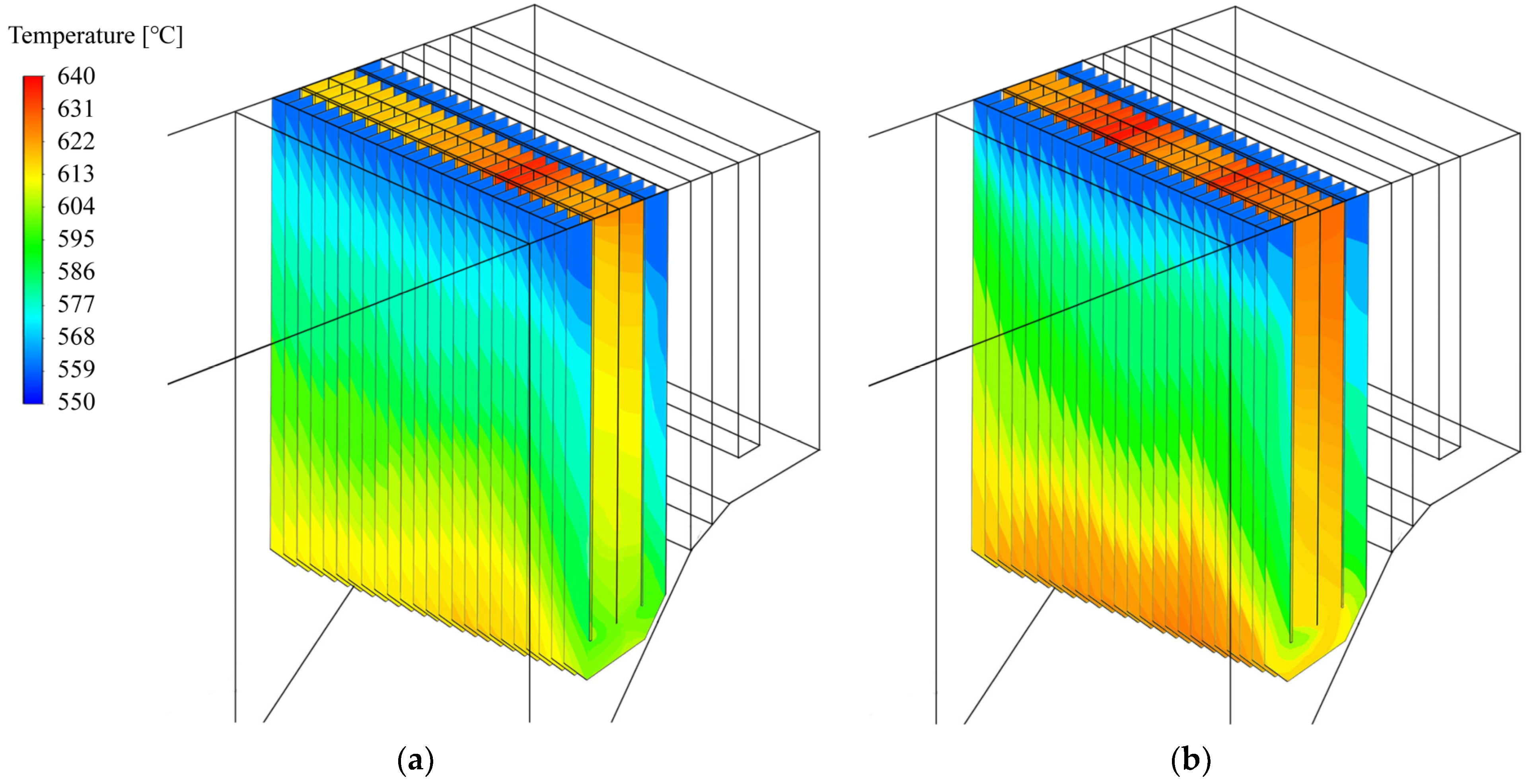
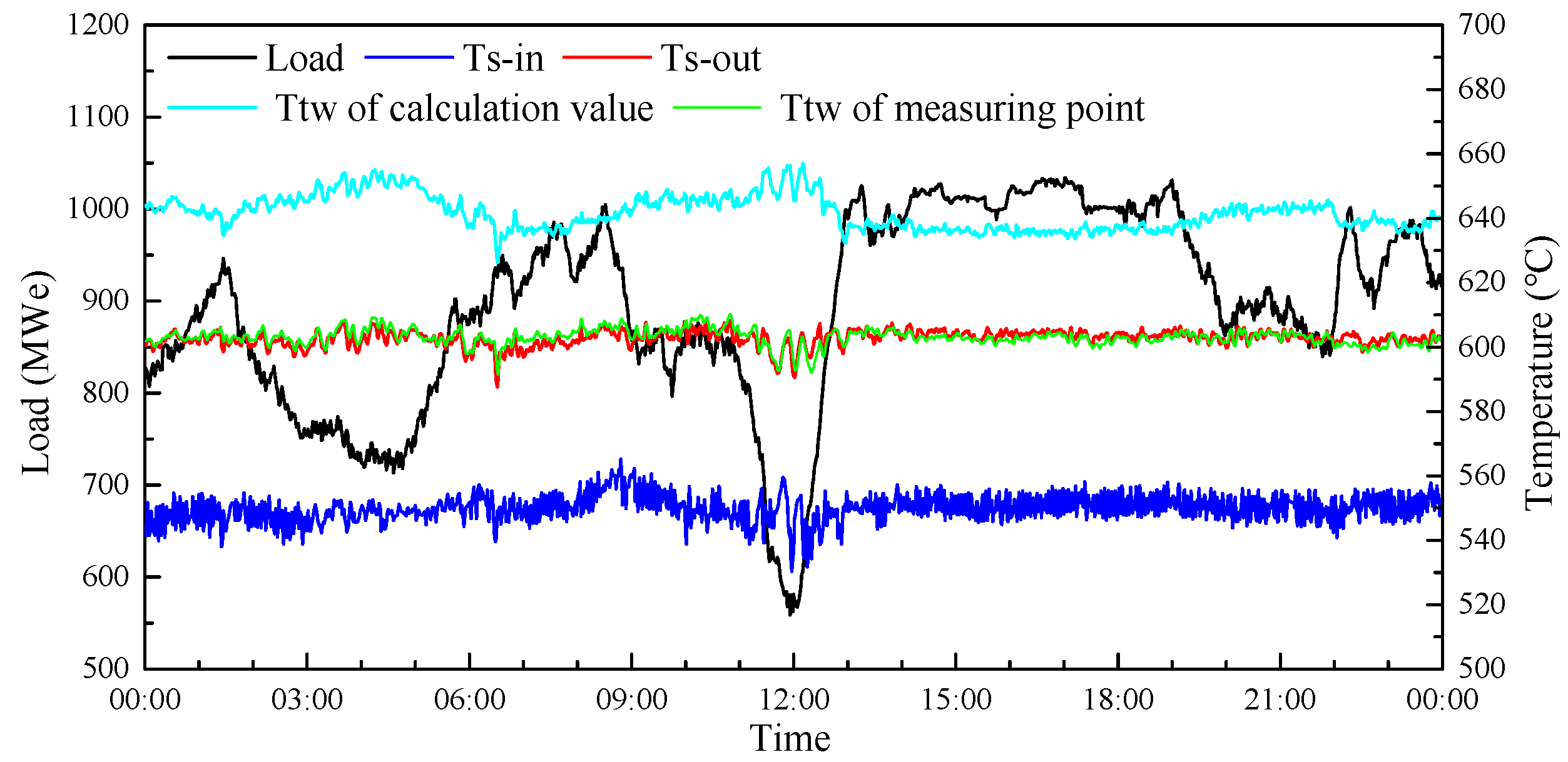
4.2. Calculation of Tube Wall Temperature

Based on the calculation method proposed in this study, an on-line monitoring system for boiler superheater tube wall temperature was developed. The system was applied to a 1000 MW USC unit. Using the operation parameters in real-time and the corresponding thermal deviation coefficient under current load, the calculated real-time tube wall temperature of FSH is displayed graphically on a web page in the form of a structure chart of the heating surface. The system records the allowable material temperatures of each tube section of the FSH, so it can automatically give alarms in case of over-temperatures in certain tube sections. The calculation results of tube wall temperatures under different boiler operation conditions are stored in a database.
Figure 10 shows the calculated results of tube wall temperature distribution in FSH under the 100 and 75% load cases. The calculated tube wall temperature distribution basically corresponded to the inlet section flue gas temperature distribution along the boiler width direction. Especially for the 75% load case, the temperature distribution on the tube wall surface and at the FSH outlet showed an obvious “M” type distribution along the furnace width, which was consistent with the flue gas temperature distribution. For a single tube platen, the tube wall temperature gradually increased from the working fluid inlet to the working fluid outlet, and the tube wall temperature at the working fluid outlet was generally the highest. These temperature distribution results are basically similar to those in reference [22]; however, the local high-temperature zone in reference [20] and reference [29] were at the bottom of the FSH. The main reason for the difference may have been due to the different position of the FSH in the boiler. The FSH in this study and in reference [22] were behind the FPSH and the RPSH, and received less radiation from the furnace, while in reference [20] and reference [29], the FSH position was closer to the furnace, and received more radiation from the furnace. This phenomenon of the temperature distribution in this study fully conforms to the law of the allowable metal temperature of the FSH metal material, and the calculated local high-temperature position was consistent with the actual over-temperature position; this had been confirmed via metal detection when the unit stopped. The tube wall temperature of the FSH for the 75% load case was higher than that for the 100% load case, which is consistent with the results of reference [29]. In other words, the tube wall temperature more easily exceeds the allowable metal temperature at lower loads. The main reason for this is that the working fluid flow rate is more sensitive to a reduction in load than the flue gas temperature, resulting in a reduction of the cooling effect of the working fluid on the tube wall.
Figure 11a shows the on-line calculated tube wall temperature distribution of the 50th tube platen in the FSH at a certain operating condition, and the position of the 50th tube platen is marked in Figure 3. Six points are marked along the flow direction of the working fluid in the serpentine pipe, from P1 to P6, in turn, as shown in Figure 11b. According to the DCS system, the inlet steam temperature (Ts-in) of the FSH was about 550 °C, and the outlet steam temperature (Ts-out) was about 600~605 °C. The calculated tube wall temperature of the FSH increased gradually along the working fluid flow path. Since the heat transfer between the tube and working fluid was much better than that between the tube and flow gas, the tube wall temperature was closer to that of the working fluid. The temperature at P1 was approximately equal to the inlet working fluid temperature. The temperature at P4 was equal to that of the outlet working fluid temperature. At P6, the tube wall temperature reached its maximum value, which was about 80 °C higher than that of P1. Meanwhile, the working fluid temperature increased only by 54 °C along the flow path.
The wall temperatures of the six feature points (Ttw-P1 to Ttw-P6) on the 50th tube platen of the FSH operating at 100 and 75% load cases are shown in Figure 12. The temperature variation trends under the two load cases were different. For the 100% load case, the tube wall temperature rose in a zigzag manner from P1 to P6. The phase in which the tube wall temperature rose was most pronounced between P3 and P4. This is not only related to the long tube distance here, but also related to the local thermal deviation condition, i.e., the high local flue gas temperature. For the 75% load case, the local high temperature zone at the inlet of the FSH moved up, and the wall temperature increased almost linearly from P1 to P6. Compared to the 100% load case, the wall temperature rose from P3 to P4 decreased for the 75% load case, while from P2 to P3 and from P4 to P5, it increased. The tube wall temperature after P3 for the 75% load case was higher than that for the 100% load case, and the difference between them was about 8 °C at P6, where the tube wall temperature reached its highest value.
The continuous 24-h on-line calculation results of the maximum tube wall temperature (at the position of working fluid outlet) of the first serpentine on the 50th tube platen of the FSH are shown in Figure 13. As a peak regulation unit, the unit load changed within the range of about 550 MW to 1035 MW. At this time, the outlet steam temperature of the FSH, i.e., the main steam temperature, was basically kept stable within the rated parameter range of 600~605 °C. The inlet steam temperature frequently changed between 530 and 565 °C. It fluctuated greatly, mainly due to the influence of spray desuperheating before the FSH inlet. Many units are designed with many tube wall temperature measuring points installed on the outlets of serpentines. These measuring points are located at the furnace top chamber above the furnace roof tube. There is no high-temperature flue gas, and the ambient temperature is only about 500 °C. Due to the influence of heat dissipation of the working fluid in the tubes, the variation trend of the temperature by measuring points is almost consistent with the outlet temperature of the working fluid. Therefore, the measured tube wall temperature does not represent the actual tube wall temperature of the heating surface in the boiler, and should not be used as the basis for judging the local over-temperature of the heating surface. The maximum tube wall temperature calculated in this study can better reflect the change in real tube wall temperature with boiler loads. On the one hand, the calculated maximum tube wall temperature was significantly higher than the outlet steam temperature and the measured tube wall temperature. On the other hand, the variation in the calculated maximum tube wall temperature with boiler loads was significantly higher than that of the outlet steam temperature and the measured tube wall temperature.

5. Conclusions

A calculation method of thermal deviation based on the combination of excess air coefficient measurement and three-dimensional full-scale numerical simulation of boiler combustion was proposed in this study. Based on the actual operating conditions of a 1000 MW coal-fired boiler, the deviation coefficient of secondary air flow of different burners was set as the boundary condition of the boiler three-dimensional full-size numerical simulation. The calculation conditions were more consistent with the actual operation states of the boiler, so that the temperature distribution of the inlet section of the FSH calculated by numerical simulation was very consistent with the measured value. Actual thermal deviation conditions along the width and vertical directions were introduced into the on-line calculation of tube wall temperature of the boiler of the FSH. The wall temperature distributions of tube platens of the FSH and the serpentines in those tube platens under boiler-continuous operation conditions were calculated. With the boiler load decreasing from 100% load to 75% load, the tube wall temperature of the FSH generally increased. Compared with previous calculation methods, the improved method has a higher level of accuracy. The calculated local high-temperature zone conformed to the law of the allowable metal temperature of the FSH serpentines segment, and was consistent with the actual over-temperature position. An on-line calculation system developed based on the current calculation method was applied to a 1000 MW USC unit. Compared with measuring temperature with thermocouples installed on the outlet of serpentines, the calculation method in this study reflects a change in real tube wall temperature more accurately. Moreover, an on-line monitoring system for boiler superheater tube wall temperature was developed based on the calculation method proposed in this study. According to the calculated local over-temperature zone, an immediate warning response from the on-line computing system can effectively help operators find the local over-temperature zone and make timely adjustments in operating parameters, thereby preventing over-temperature BTF.

Author Contributions

Conceptualization, T.B. and Y.Z.; methodology, P.L.; validation, Z.S.; formal analysis, W.Z.; investigation, P.L.; resources, J.G.; data curation, Z.S.; writing—original draft, P.L.; writing—review and editing, T.B. and W.Z.; visualization, Z.S. and Y.Z.; supervision, J.G.; project administration, T.B. and Z.X.; funding acquisition, Z.X. All authors have read and agreed to the published version of the manuscript.

Funding

This study was supported by the Science and Technology Program of “System Development of Safety State Assessment System for High-temperature Heating Surface of Ultra-supercritical Boilers Based on Inner Wall Temperature Monitoring” of Zhejiang Province Energy Group Co., Ltd.

Data Availability Statement

The data presented in this study are available on request from the corresponding author. The data are not publicly available due to the confidentiality of the data.

Acknowledgments

The authors gratefully acknowledge Zhejiang Energy Group Co., Ltd., Zhejiang Zheneng Zhongmei Zhoushan Coal & Electricity Co., Ltd. and Zhejiang Zheneng Technology Research Institute Co., Ltd. for utilization of all the facilities and resources.

Conflicts of Interest

The authors declare no conflict of interest.

References

  1. BP. BP Statistical Review of World Energy 2021; BP Amoco: London, UK, 2021. [Google Scholar]
  2. China Electricity Council P A S. Available online: https://cec.org.cn/detail/index.html?3-308855 (accessed on 2 October 2022).
  3. Tan, P.; Fang, Q.; Zhao, S.; Yin, C.; Zhang, C.; Zhao, H. Causes and mitigation of gas temperature deviation in tangentially fired tower-type boilers. Appl. Therm. Eng. 2018, 139, 135–143. [Google Scholar] [CrossRef]
  4. Xu, L.; Khan, J.; Chen, Z. Thermal load deviation model for superheater and reheater of a utility boiler. Appl. Therm. Eng. 2000, 20, 545–558. [Google Scholar] [CrossRef]
  5. Huang, J.; Zhou, K.; Xu, J.; Bian, C. On the failure of steam-side oxide scales in high temperature components of boilers during unsteady thermal processes. J. Loss Prevent. Proc. 2013, 26, 22–31. [Google Scholar] [CrossRef]
  6. French, D.; Vedhara, K.; Kaptein, A.; Weinman, J. Metallurgical Failures in Fossil Fired Boilers; John Wiley & Sons, Inc.: New York, NY, USA, 1993. [Google Scholar]
  7. Dooley, B. Don’t let those boiler tubes fail again: Part 2. Power Eng. 1997, 101, 56–61. [Google Scholar]
  8. Kuznetsov, N.; Mitor, W.; Dubovski, I.; Karasina, E. Thermal Calculations of Steam Boilers (Standard Method); Standard Method, Energy: Moscow, Russian, 1973. (In Russian) [Google Scholar]
  9. Wagner, W.; Cooper, J.; Dittmann, A.; Kijima, J.; Kretzschmar, H.; Kruse, A. The IAPWS industrial formulation 1997 for the thermo-dynamic properties of water and steam. J. Eng. Gas. Turb. Power 2000, 1, 150–184. [Google Scholar] [CrossRef]
  10. Wang, M.; Shao, W.; He, P.; Wang, Z.; Yang, Z. Temperature Imbalances in Convection Superheater and Reheater Panels of Utility Boiler. Power Eng. 1984, 02, 41–48. (In Chinese) [Google Scholar]
  11. Wang, M.; Yang, Z.; He, P. Shooting Temperature Difference in Platen Type Superheater Panels. Power Eng. 1986, 06, 18–26. (In Chinese) [Google Scholar]
  12. Prieto, M.; Suárez, I.; Fernández, F.; Sánchez, H.; Mateos, M. Theoretical development of a thermal model for the reheater of a power plant boiler. Appl. Therm. Eng. 2007, 27, 619–626. [Google Scholar] [CrossRef]
  13. Madejski, P.; Taler, D.; Taler, J. Numerical model of a steam superheater with a complex shape of the tube cross section using Control Volume based Finite Element Method. Energ. Convers. Manag. 2016, 118, 179–192. [Google Scholar] [CrossRef]
  14. Taler, D.; Trojan, M.; Taler, J. Mathematical modeling of cross-flow tube heat exchangers with a complex flow arrangement. Heat. Transfer. Eng. 2014, 35, 1334–1343. [Google Scholar] [CrossRef]
  15. Taler, D.; Trojan, M.; Dzierwa, P.; Kaczmarski, K.; Taler, J. Numerical simulation of convective superheaters in steam boilers. Int. J. Therm. Sci. 2018, 129, 320–333. [Google Scholar] [CrossRef]
  16. Trojan, M. Modeling of a steam boiler operation using the boiler nonlinear mathematical model. Energy 2019, 175, 1194–1208. [Google Scholar] [CrossRef]
  17. Trojan, M.; Taler, D. Thermal simulation of superheaters taking into account the processes occurring on the side of the steam and flue gas. Fuel 2015, 150, 75–87. [Google Scholar] [CrossRef]
  18. Xu, H.; Deng, B.; Jiang, D.; Ni, Y.; Zhang, N. The finite volume method for evaluating the wall temperature profiles of the superheater and reheater tubes in power plant. Appl. Therm. Eng. 2017, 112, 362–370. [Google Scholar] [CrossRef]
  19. Sun, L.; Yan, W. Prediction of wall temperature and oxide scale thickness of ferritic–martensitic steel superheater tubes. Appl. Therm. Eng. 2018, 134, 171–181. [Google Scholar] [CrossRef]
  20. Laubscher, R.; Rousseau, P. CFD study of pulverized coal-fired boiler evaporator and radiant superheaters at varying loads. Appl. Therm. Eng. 2019, 160, 114057. [Google Scholar] [CrossRef]
  21. Gómez, A.; Fueyo, N.; Díez, L. Modelling and simulation of fluid flow and heat transfer in the convective zone of a power-generation boiler. Appl. Therm. Eng. 2008, 28, 532–546. [Google Scholar] [CrossRef]
  22. Akkinepally, B.; Shim, J.; Yoo, K. Numerical and experimental study on biased tube temperature problem in tangential firing boiler. Appl. Therm. Eng. 2017, 126, 92–99. [Google Scholar] [CrossRef]
  23. Zhou, Y.; Li, P.; Ao, X.; Zhao, H. High temperature corrosion inhibition for opposed firing boiler based on combustion distribution evenness. J. Zhejiang Univ.-ES 2015, 49, 1768–1775. (In Chinese) [Google Scholar] [CrossRef]
  24. Wang, Z.; Wu, W.; Li, H. Real-time measurement methods for flue gas temperature at furnace outlet in large scale power plants. Therm. Power Gener. 2016, 45, 74–80. (In Chinese) [Google Scholar] [CrossRef]
  25. Laubscher, R.; Rousseau, P. Numerical investigation on the impact of variable particle radiation properties on the heat transfer in high ash pulverized coal boiler through co-simulation. Energy 2020, 195, 117006. [Google Scholar] [CrossRef]
  26. Liu, H.; Liu, Y.; Yi, G.; Nie, L.; Che, D. Effects of air staging conditions on the combustion and NOx emission characteristics in a 600 MW wall fired utility boiler using lean coal. Energ. Fuel 2013, 27, 5831–5840. [Google Scholar] [CrossRef]
  27. Yu, Y.; Liao, H.; Wu, Y.; Zhong, W. Study on tube wall temperature of power plant boilers based on coupled thermal hydraulic analysis. J. Chin. Soc. Power Eng. 2015, 35, 1–7. (In Chinese) [Google Scholar] [CrossRef]
  28. Wu, X.; Fan, W.; Liu, Y.; Bian, B. Numerical simulation research on the unique thermal deviation in a 1000 MW tower type boiler. Energy 2019, 173, 1006–1020. [Google Scholar] [CrossRef]
  29. Jin, D.; Liu, X.; Zhang, X.; Shen, Y.; Wang, T.; Li, C.; Li, X.; Wei, J.; Fu, J.; Wang, H. A coupled model for prediction the tube temperature of platen superheater of coal-fired boiler. Proc. CSEE 2022, 1–13. [Google Scholar] [CrossRef]
Figure 1. Layout of burners and high-temperature heating surfaces of the 1000 MW USC coal-fired boiler.
Energies 16 01539 g001
Figure 2. The metal material, pipe specifications, and allowable temperatures of the FSH.
Energies 16 01539 g002
Figure 3. Layout of flue gas temperature measuring points on the inlet flue section of the FSH.
Energies 16 01539 g003
Figure 4. Grid system of the 1000 MW USC boiler.
Energies 16 01539 g004
Figure 5. Numerical simulation results and design values of flue gas temperatures in different cross sections.
Energies 16 01539 g005
Figure 6. Excess air coefficient distribution along the width direction of the boiler.
Energies 16 01539 g006
Figure 7. Numerical simulation results of flue gas temperature contours; (a) 100% load case; (b) 75% load case.
Energies 16 01539 g007
Figure 8. Flue gas temperature contours at the inlet of the FSH from numerical simulation and measuring points; (a) numerical simulation results for the 100% load case; (b) numerical simulation results for the 75% load case; (c) measured results for the 100% load case; (d) measured results for the 75% load case.
Energies 16 01539 g008
Figure 9. Thermal deviation coefficient of 5 vertical regions.
Energies 16 01539 g009
Figure 10. Calculated results of tube wall temperature distribution of the FSH; (a) 100% load case; (b) 75% load case.
Energies 16 01539 g010
Figure 11. Calculation results of the temperature distribution of serpentine and feature points locations; (a) tube wall temperature distribution of serpentine; (b) locations of P1 to P6.
Energies 16 01539 g011
Figure 12. Tube wall temperature variation along the steam flow under two different load cases.
Energies 16 01539 g012
Figure 13. Tube wall temperature calculation results over 24 h.
Energies 16 01539 g013
Table 1. Operating conditions of the boiler for 100% and 75% load cases.
ParameterDesign Conditions (BMCR)Actual Operating Condition
100% Load75% Load
Mills in serviceABCDEABCDEFABCDE
Total coal flow rate (kg/s)106.3995.0771.30
Primary air flow rate (kg/s)189.72179.12141.74
Primary air inlet temperature (°C)70.073.877.2
Secondary air flow rate (kg/s)392401327
Secondary air inlet temperature (°C)354342328
Inner secondary air rate (%)303030
Outer secondary air rate (%)707070
Sofa air flow rate (kg/s)142.6136.176.3
Sofa air inlet temperature (°C)354342328
Disclaimer/Publisher’s Note: The statements, opinions and data contained in all publications are solely those of the individual author(s) and contributor(s) and not of MDPI and/or the editor(s). MDPI and/or the editor(s) disclaim responsibility for any injury to people or property resulting from any ideas, methods, instructions or products referred to in the content.

