Comparative Analysis of Eight Numerical Methods Using Weibull Distribution to Estimate Wind Power Density for Coastal Areas in Pakistan

Abstract

Currently, Pakistan is facing severe energy crises and global warming effects. Hence, there is an urgent need to utilize renewable energy generation. In this context, Pakistan possesses massive wind energy potential across the coastal areas. This paper investigates and numerically analyzes coastal areas’ wind power density potential. Eight different state-of-the-art numerical methods, namely an (a) empirical method, (b) graphical method, (c) wasp algorithm, (d) energy pattern method, (e) moment method, (f) maximum likelihood method, (g) energy trend method, and (h) least-squares regression method, were analyzed to calculate Weibull parameters. We computed Weibull shape parameters (WSP) and Weibull scale parameters (WCP) for four regions: Jiwani, Gwadar, Pasni, and Ormara in Pakistan. These Weibull parameters from the above-mentioned numerical methods were analyzed and compared to find an optimal numerical method for the coastal areas of Pakistan. Further, the following statistical indicators were used to compare the efficiency of the above numerical methods: (i) analysis of variance ($R^2$), (ii) chi-square ($X^2$), and (iii) root mean square error (RMSE). The performance validation showed that the energy trend and graphical method provided weak performance for the observed period for four coastal regions of Pakistan. Further, we observed that Ormara is the best and Jiwani is the worst area for wind power generation using comparative analyses for actual and estimated data of wind power density from four regions of Pakistan.

1. Introduction

Energy is essential for every system in the world to maintain its existence. In this context, the requirement for energy is increasing over time with technological developments and population growth [1,2,3]. Accordingly, searching for available renewable energy resources (RERs) has become a significant problem because RERs are a considerable factor affecting any country’s economic shape. RERs are not only considered internal dynamics of nations but also a critical factor that influences countries that are experiencing political and military clashes. As is known, RERs are also a fundamental part of social and economic developments in every society [4,5]. Wind energy (WE) is an environmentally friendly energy resource used for irrigation, vessels, wheat grinding, and several other fields. Wind energy seems to be a good substitute for fossil fuels that could contribute to the development of the economy in the upcoming time. Nations will use RERs rather than fossil fuels to meet energy requirements using efficient integration and demand-side management [6,7,8]. In [9], the authors presented a brief overview of recent developments in wind energy potentials, wind energy curtailments, mismatches between the installed energy capacities and generated energy, policies, investments, and the prospects and impacts of wind energy developments in China. From 1969 to 2016, the involvement of Mexican institutes in the literature specialized on wind energy was analyzed in [10].

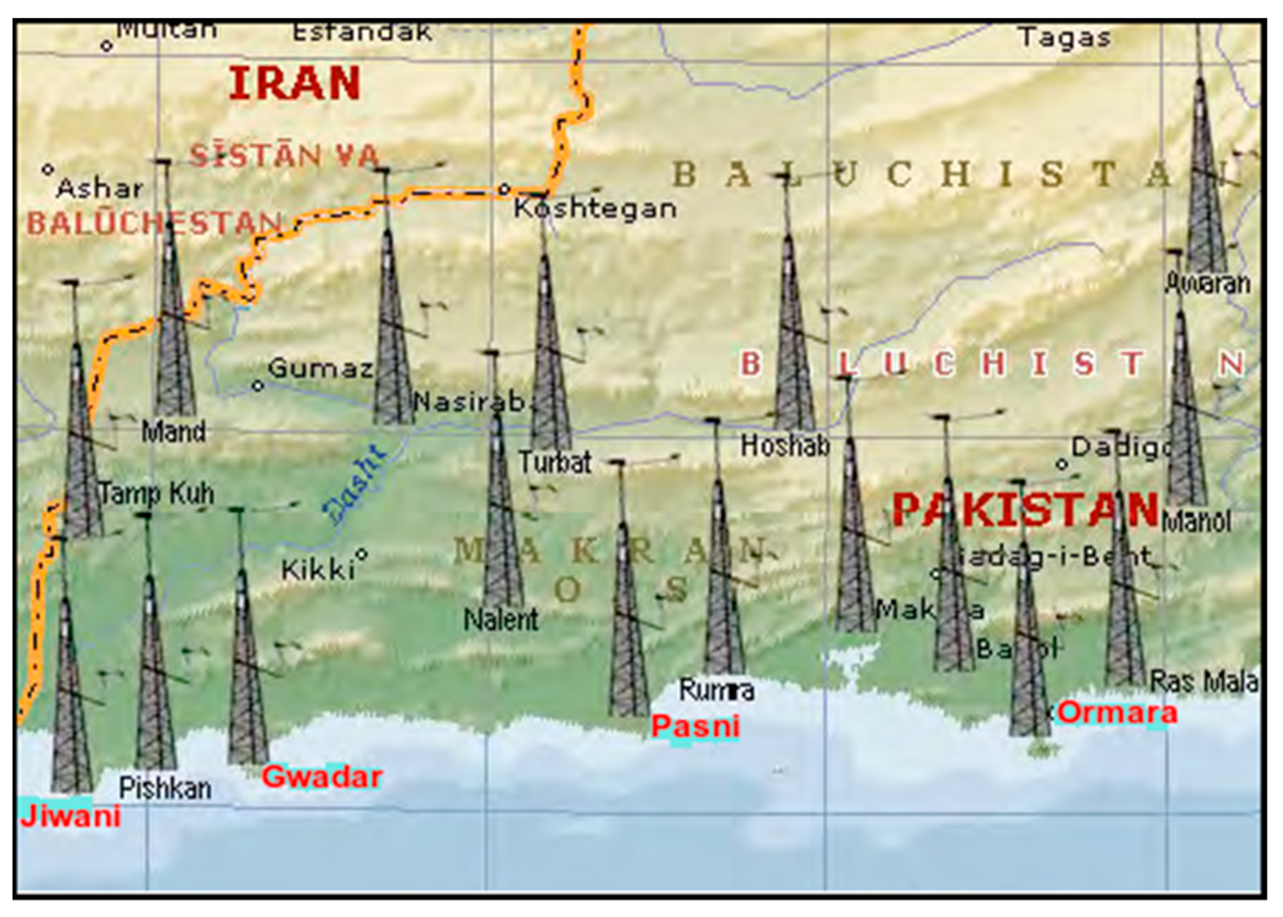
The year-wise growth and capacity of wind power in Pakistan are presented in

Table 1. Annual production capacities and growth of wind power in Pakistan.

Year	Capacity (MW)	Growth (MW)	Growth (%)
2007	0	0	-
2008	6	6	-
2009	6	0	-
2010	6	0	-
2011	6	0	-
2012	56	50	+833.4
2013	106	50	+89.3
2014	256	150	+141.6
2015	256	0	-
2016	591	335	+130.9
2017	789	198	+33.6
2018	1186	397	+50.4
2019	1236	50	+4.3
2020	1236	0	-
2021	1335	99	+8.1

. When wind energy plants were connected to the central grid for the first time in Pakistan, 8 megawatts (MW) of wind power was supplied and zero growth followed for the next three years. After 2011, a dramatic increase happened until 2019 due to rising interest in renewable energies worldwide. The highest growth was observed in 2012, 2014, and 2016 [11]. Moreover, the Ministry of Energy (Pakistan) expects that annual installation of wind energy plants will increase year by year. In [12], the authors discussed the future success and current scenario of RERs for under-construction and operational RER projects such as wind energy, solar energy, biogas, biomass, and hydropower, along with the role of institutions and organizations in the RER field. The proposed wind energy sites in Pakistan are shown in Figure 1. In [13], the authors explored sites for wind farm installations in a coastal area of Pakistan. The total area of Pakistan is $796,095 {\mathrm{Km}}^2$ including $77,085 {\mathrm{Km}}^2$ area with water regions. Pakistan’s total coastal line length is 1100 km, while the wind zone area is 250 km. In this paper, the authors considered four coastal areas of Baluchistan to estimate wind power density (WPD) in these regions, as shown in Figure 1.

Evaluating the economic feasibility of wind projects is particularly challenging due to the wind’s intermittent nature and the high sensitivity of project profitability to various parameters. This highlights the importance of uncertainty analysis in the wind power industry. A combination of sensitivity analysis and the Monte Carlo method for a technical and economic model of a wind farm assisted in better understanding the impact of uncertainties on the financial risks of wind projects [14]. Wind farms can be fully exploited based on a detailed representation of statistical characteristics to find the exact wind turbine type and configuration. This resulted in a clear relation between the error of a Weibull distribution and an estimation error of wind energy generation. Therefore, selecting a suitable distribution function is pivotal in choosing the correct wind turbines and maximizing wind energy production [15]. Therefore, carefully selecting estimation functions is critical in accurately calculating cost analysis and determining optimal wind turbines. In this regard, we examined eight numerical methods for four sites possessing enormous wind energy potential. This work will provide guidance to future project designers to accurately determine the cost analysis and extract the maximum wind energy using an appropriate method.

Widely adopted PDFs are unimodal types, including Weibull, Rayleigh, exponential, Gauss, gamma, and lognormal functions [16]. The two-parameter Weibull distribution (WD) function is commonly used to calculate WE characteristics and represent wind speed. As it is more general than the Rayleigh, the Gauss, and exponential functions, it typically performs better than the lognormal function [17]. Overall, the gamma function performs similarly to the Weibull function. Still, it presents the disadvantage that the analytical expression of the mean, variance, skewness, and kurtosis of the wind power PDF cannot be determined [18]. Recent literature also proposes a mixture of functions of unimodal distributions, such as the two-component mixture. In [19], it is described that when there are two peaks in the wind regime, using a mixture of functions or a maximum entropy function provides a better characterization of wind than using the conventional Weibull function alone. However, this is not the case in the current study.

Different numerical methods have been proposed in the literature to estimate WD parameters. The authors in [20] used the wind speed data of different time spans (daily, monthly, and annually) during a period of five and a half years (5.5 years) to estimate the Weibull s parameter (WSP), Weibull scale parameter (WCP), and wind probability density distribution at 30, 50, and 70 m height in Alacati, Turkey. In [21], the authors reviewed and analyzed different methods, such as the empirical, graphical, momentary, and maximum likelihood. A comparative assessment of offshore wind energy potential was provided using six different numerical methods for calculating WPD [22]. The authors of [23] estimated Weibull distribution parameters at low wind speeds considering six numerical methods for a selected region. In [24], the authors provided a comparative analysis of six numerical methods to calculate the coefficient of the Weibull distribution function at two different heights. The standard deviation method was applied to determine Weibull parameters considering various potential sites for performance analysis [25]. The authors of [26] used a technique called four moments mixture for WPD estimation in wind estimation applications. In [27], the authors utilized various numerical methods to estimate the potential of the sites Mersing and Port Dickson in Malaysia. The authors of [28] compared the performance of numerical methods used to calculate Weibull parameters for Cameroon. Different numerical methods were analyzed and compared concerning their performance to determine WCP and WSP for Weibull distributions from 2011 to 2015 for six coastal regions in Morocco [29]. The authors of [30] measured wind speed (WS) at three different heights and calculated the WD parameters (shape and scale) to evaluate the wind speed characteristics and wind energy potential at seven locations in Cameroon. In [31], five different numerical methods were analyzed: the maximum likelihood method, EM, EPM, GM, and modified MLM, and their performance was compared to determine the effectiveness of WD parameters. The authors of [32,33] provided a comparative analysis of various methods to determine Weibull PDFs. Moreover, the performance of multiple methods was analyzed for specific locations to determine the best possible method to determine the Weibull parameters accurately [34,35].

Our literature review provided various estimation methods applied to different datasets but showed no superior method compared to other methods considering the available datasets and probabilistic representation. Therefore, an estimation method must adhere to the available dataset and estimation functions to extract the maximum wind power generation. To this end, we attempted to analyze the various potential sites using multiple methods and provide the best possible outcome regarding maximized wind generation and reduced associated costs.

The works mentioned above successfully estimated Weibull parameters using six numerical methods and considered various potential sites. However, our work provides a comparative analysis of eight numerical methods to estimate the WPD of coastal areas of Pakistan. In this paper eight different numerical methods, an (a) empirical method, (b) graphical method, (c) wind atlas analysis and application program algorithm, (d) energy pattern method, (I) moment method, (f) least squares regression method, (g) maximum likelihood method, and (h) energy trend method, were analyzed to find the Weibull parameters, namely WSP and WCP, for the four regions Jiwani, Gwadar, Pasni, and Ormara. Further, we estimated the WE potential using WS, wind direction, and other data from coastal areas of Pakistan during a six-year period (2011–2016) which were obtained from the meteorological office in Karachi. Moreover, the best numerical method was determined by using the statistical indicators (i) analysis of variance ($R^2$), (ii) root mean square error (RMSE), and (iii) chi-square ($X^2$). The authors of the present study also estimated annual mean wind speed (MWS), standard deviation (SD), and mean WPD densities for the respective areas of Pakistan. Lastly, we determined the best WE site in the analyzed regions.

Considering the above discussion, our work’s pertinent contributions are as follows:

• Various methods are comparatively analyzed considering the specific dataset of Pakistan’s mentioned potential wind energy sites.
• Our comparative analysis provides insight into the best method concerning the available dataset, i.e., the method that results in maximum wind energy extraction from the mentioned sites.
• The proposed methods are explained in detail for available datasets and sites to provide the best possible results regarding maximized energy production.
• Finally, the best possible method is determined for each potential site, the one that achieved the maximum energy production, which is discussed in detail in the results section. This provides evidence for the best possible method for each location.

The remainder of our paper is organized as follows: Details of the Weibull distribution function, probability distribution function, cumulative distribution function, and wind power density calculation are discussed in Section 2. In Section 3, eight different numerical methods are analyzed. The critical discussion of results is listed in Section 4. A summary and a proposal for future work are discussed in Section 5.

2. Weibull Distribution Function (WDF)

Wind energy is more diffuse and has a more variable flux than other renewable resources, such as solar or tidal energy. To maximize wind energy benefits, the description of variation in wind velocity at a specific site is essential; it plays a significant role in developing wind energy conversion technology [30]. The WDF gives us an accurate approximation of natural phenomena to apply the laws of probability. It helps find the speed distribution of wind for studying the load analysis of wind. Recently this method has received great attention and focus from the application perspective of wind energy; not only because of its greater flexibility and simplicity but also due to its best fit to experimental data. WDF is classified into two main types, the cumulative distribution function and the probability distribution function [36].

2.1. Probability Distribution Function (PDF)

The WD function is a two-parameter function characterized by a WCP and WSP. These two parameters help find the WS, which gives us the optimum level of performance for a wind conversion system It also provides the range of speed over which the device operates and can be represented as

$$f\left(v\right)=\frac{k}{v}{\left(\frac{v}{c}\right)}^{k-1}{e}^{\left(-{\left(\frac{v}{k}\right)}^k\right)}$$

(1)

where $c$, $k$, and $v$ represent WCP, WSP, and WS, respectively.

2.2. Cumulative Distribution Function (CDF)

Integration of the WD function is called CDF, which shows the integration and cumulation of relative frequency for each velocity interval. The equation of the CDF can be presented as follows:

$$F\left(v\right)=1-e^{-{\left(\frac{v}{c}\right)}^k.}$$

(2)

2.3. Wind Power Density (WPD)

To benefit from WE, it is necessary to determine the WPD. The mathematical expression for WPD is as follows [30]:

$$P_w=\frac{1}{2} \left(\rho A{v}^3\right),$$

(3)

where $P_w$ is the WPD potential, A is the swept area of a wind turbine, $\rho$is the air density, and $v$ is the WS. The WPD is highly dependent on the WS (3). While WS is vital in calculating the WPD, wind direction also plays a significant role in installing wind farms. Moreover, specific time intervals of wind velocity are also crucial for a region to detect WPD potential. Several functions are used for calculating the dispersion of WS, whereby the two-parameter WD function is the most used [30].

3. Evaluation of Weibull Parameters

The shape parameter of a Weibull distribution is crucial for investigating and finding the characteristics of wind waves at a site. The Weibull scale factor shows the WPD potential of that spot. The larger the value of the WCP, the higher the wind potential. These two parameters of the WD function affect the distribution curve; therefore, these parameters should be considered collectively for determining the characteristics of a region’s wind. Different methods are used to determine the parameters of the WD function, as justified by various studies [25]. Here we will discuss eight numerical methods, i.e., an (a) empirical method, (b) graphical method, (c) wind atlas analysis and application program algorithm, (d) energy pattern method, (e) moment method, (f) least squares regression method, (g) maximum likelihood method, and (h) energy trend method.

3.1. Graphical Method (GM)

One of the main advantages of using a graphical method is that it can provide a clear and intuitive way to understand the characteristics of wind speed data. Using the Weibull distribution in combination with graphical methods, such as probability plots, can provide a more comprehensive understanding of the data and how well it fits the Weibull model, which can be very useful in understanding the reliability of a system or product and making predictions about future failures. Therefore, a GM is used with the Weibull distribution function [36]. In this method, a graph is constructed so that a straight line is drawn and built for a cumulative WD, where the shape factor shows its slope. Taking the logarithm of (2), we get the following expression [28]:

$$-\mathit{ln}\left\{1-F\left(v\right)\right\}=klnv-klnc.$$

(4)

The relation between $lnv$ and $-\mathit{ln}\left\{1-F\left(v\right)\right\}$ is shown in (4). We plot so the horizontal axis of this graph from a Weibull paper is v while on the vertical axis, we have $ln{\left(1-F\left(v\right)\right)}^{-1}$. We get a straight line as a result, with a slope “k”. While plotting the Weibull distribution, v is along the vertical axis and $ln{\left(1-F\left(v\right)\right)}^{-1}$ is along the horizontal axis.

3.2. Empirical Method (EM)

The main advantage of using an empirical method in research is that it relies on observation and experimentation to gather data and test hypotheses, which can provide strong evidence for or against a theory or claim. An empirical method’s main benefit is collecting reliable and valid data, which can be used to test hypotheses and establish causal relationships. EM provide a comprehensive understanding of the data and the underlying processes that generated them, which can be valuable in making predictions, design decisions, and improving the performance of a system or product. In this regard, use of EM is considered to evaluate the Weibull distribution function [5,36]. In EM, data distribution permits the resolution of the relation between the mean WS value and SD values between the WSP numerical methods used to compute the WSP and the WCP. WCP and WSP can be presented as follows [5,36]:

$$k={\left(\frac{\overline{v}}{\sigma }\right)}^{1.086}$$

(5)

$$c=\frac{\overline{v}}{\mathrm{ᴦ}\left(1+\frac{1}{k}\right)}$$

(6)

$$\overline{v}=\frac{1}{n}{\displaystyle \sum }_{i=1}^n{v}_i$$

(7)

$$\sigma =\sqrt{\frac{1}{n}{\displaystyle \sum }_{i=1}^n\left(v_i-v_m\right)}$$

(8)

where “$\sigma$” represents the variance, “$\overline{v}$” represent the mean WS, and “ᴦ” shows the gamma function.

3.3. Energy Pattern Method (EPM)

The energy pattern method’s primary purpose is to identify areas of high and low wind speeds within a specific region, which can help identify the most promising locations for wind energy development. The method can also be used to analyze the effect of topographical features such as mountains, lakes, and coastlines on wind patterns. This information can be used to optimize wind turbine placement and improve the efficiency of wind energy projects. The main advantage of the EPM is to identify patterns and relationships in the dataset, which can be used to make predictions and forecasts about future usage. By analyzing patterns in historical data, the EPM can help to identify trends and forecast the future. Additionally, it could also be used for simulation and energy optimization by including probability distributions so that the EPM can provide a comprehensive way of dealing with the randomness and uncertainty of the datasets. The EPM calculates the mean wind speed [36]. The mean of the WS cubes and the cube of the MWS are used in this method to calculate the WSP, WCP, and energy pattern factor ”$E_{PF}$” in [36].

$$E_{PF}=\frac{\left(\frac{1}{n}\right){{\displaystyle \sum }}_1^n{v}_i^3}{{(\left(\frac{1}{n}\right){{\displaystyle \sum }}_1^n{v}_i)}^3}$$

(9)

$$k=1+\frac{369}{E_{PF}^2}$$

(10)

$$c=\frac{v_m}{\mathrm{ᴦ}\left(1+\frac{1}{k}\right)}$$

(11)

3.4. Moment Method (MM)

One of the main advantages of using the moment method for wind speed data is that it can provide a simple and efficient way to describe the wind speed variability at a specific location. The method can estimate the mean, standard deviation, skewness, and kurtosis of the wind speed distribution, providing valuable information about the wind speed characteristics at a particular site. The moment method is a statistical technique used to estimate the parameters of a Weibull distribution, a common probability distribution used to model wind speeds. The Weibull distribution is often used because it can model both the mean and the variability of wind speeds and account for the skewness and kurtosis of the data. The moment method uses the sample mean, sample standard deviation, sample skewness, and kurtosis to estimate the parameters of the WD of wind speeds [28]. Further, the MM is the classical method to find out WDF parameters. The WSP and WCP are computed from the first two moments of the WDF. These calculations are based on the average velocity of wind, WCP, and gamma function [36]

$$k={\left(\frac{0.9874}{\sigma /v_m}\right)}^{1.0983}$$

(12)

$$c=\frac{v_m}{\mathrm{ᴦ}\left(1+\frac{1}{k}\right)}$$

(13)

where “$\sigma$” shows the WCP.

3.5. Energy Trend Method (ETM)

In the context of wind energy systems, using the ETM to analyze wind speed data can provide insights into the temporal behavior of the wind. This can be useful in understanding the expected wind speeds at different times of the year, which can be valuable information for wind turbine design and operation [5]. Moreover, in the ETM, the WCP is calculated in the same way as in the maximum likelihood method MLM. The below mathematical equation can obtain the WSP after finding the energy pattern factor ($E_{PF}$) [5]:

$$E_{PF}=\frac{\left(\frac{1}{n}\right){{\displaystyle \sum }}_1^n{v}_i^3}{{(\left(\frac{1}{n}\right){{\displaystyle \sum }}_1^n{v}_i)}^3}$$

(14)

$$k=\frac{1}{3.9557E_{PF}^{o.898}}$$

(15)

$$c={\left(\frac{1}{n}{\displaystyle \sum }_{i=1}^n{v}_i^k\right)}^{\frac{1}{k}}$$

(16)

3.6. Least Squares Regression Method (LSRM)

The goal of the LSRM is to find the line (or hyperplane) that minimizes the sum of the squared distances between the predicted values and the actual values in the data set. The LSRM can be used to model the relationship between wind speed and other variables, such as wind direction, temperature, and air pressure. Fitting a line to the data using the LSRM can help to predict wind speeds at a particular location or time based on the values of these other variables. Some benefits of the LSRM include its relative simplicity and ease of interpretability and its robustness to outliers in the data. The LSRM also can handle multiple independent variables and model non-linear relationships.

Taking a double log of (1), we can obtain the following:

$$\mathit{ln}\left[-\mathit{ln}\left(1-f\left(v\right)\right)\right]=kln\left(c\right)$$

(17)

The above linear equation can be fitted using the LSRM [31,37]. The CDF F(v) can be calculated easily using an estimator, the median rank. The WCP and WSP of WD can be estimated as follows:

$$k=\frac{n{{\displaystyle \sum }}_{i=1}^{n}lnv xln\left[-\mathit{ln}\left\{1-F\left(v\right)\right\}\right]-{{\displaystyle \sum }}_{i=1}^{n}lnv x{{\displaystyle \sum }}_{i=1}^{n}ln\left[=\mathit{ln}\left\{1-F\left(v\right)\right\}\right]}{n{{\displaystyle \sum }}_{i=1}^{n}ln{v}^2-{\left\{{{\displaystyle \sum }}_{i=1}^{n}lnv\right\}}^2}$$

(18)

$$c={\left[\frac{1}{n}{\displaystyle \sum }_{i=1}^n{v}_i^k\right]}^{\frac{1}{k}}$$

(19)

3.7. WAsP Algorithm (WAsPA)

The WAsP (Wind Atlas Analysis and Application Program) algorithm is a tool used to model the wind resources at a specific location and predict the energy production of a wind farm. The WAsPA uses atmospheric boundary layer (ABL) and wind flow modeling to predict the long-term wind speed and direction at a specific site. One of the main benefits of the WAsP algorithm is its ability to consider the complex topographical and meteorological conditions that can affect wind patterns at a specific location. The WAsPA uses detailed terrain data and statistical models of wind flow to provide highly accurate predictions of wind resources and energy production [37]. The primary two requirements for the WAsPA are (a) the WPD of the fitted WD is the same as of the observed WPD and (b) the average values are the same for both the observed WD as well as fitted WD. The relation between observed and average proportional values is as follows:

$$X=1-F\left(v\right)$$

(20)

where “X” shows the proportional values for the observed WS greater than the average WS. The CDF F(v) estimates the proportional values that are smaller than v, whereas 1 − F(v) calculates the proportional values that are greater than v, while the MWS is represented in Equation (21).

$$\overline{v}=c\mathrm{ᴦ}\left(\frac{1}{k}+1\right)$$

(21)

For fulfilling the second requirement of the WAsPA we substitute (21) in (2) to obtain the following equation

$$X=exp\left[-\mathrm{ᴦ}{\left(\frac{1}{k}+1\right)}^k\right]$$

(22)

which can be expressed as

$$-lnX=\mathrm{ᴦ}{\left(\frac{1}{k}+1\right)}^k$$

(23)

In performing the WAsPA to fit, the WD, windo-grapher 5 software determined X and solved Equation (23) iteratively, using Brent’s method to calculate the WSP [37].

3.8. Maximum Likelihood Method (MLM)

The MLM is a statistical technique used to estimate the parameters of a probability distribution that best fit a set of observed data. In wind speed, the MLM can estimate the parameters of a probability distribution that describe the wind speeds at a particular location. For example, a commonly used probability distribution for wind speeds is the Weibull distribution, often used to model wind speeds in the wind energy industry. By using the MLM to estimate the parameters of the Weibull distribution, it is possible to make accurate predictions of future wind speeds at a given location [27]. The maximum likelihood estimation approach is a mathematical statement recognized as the WD of a period of WS data [27]. In the MLM, numerical iterations are required to calculate the WCP and WSP of the WD. The parameters WCP and WSP of the WD are computed through the following equations:

$$k={\left(\frac{{{\displaystyle \sum }}_1^n{v}_i^k\mathit{ln}\left(v_i\right)}{{{\displaystyle \sum }}_1^n{v}_i^k}-\frac{{{\displaystyle \sum }}_1^{n}ln\left(v_i\right)}{n}\right)}^{-1}$$

(24)

$$c={\left(\frac{1}{n}{\displaystyle \sum }_1^n{v}_i^k\right)}^{1/k}$$

(25)

4. Critical Analysis of Results

4.1. Wind Speed (WS) Statistics from All Regions

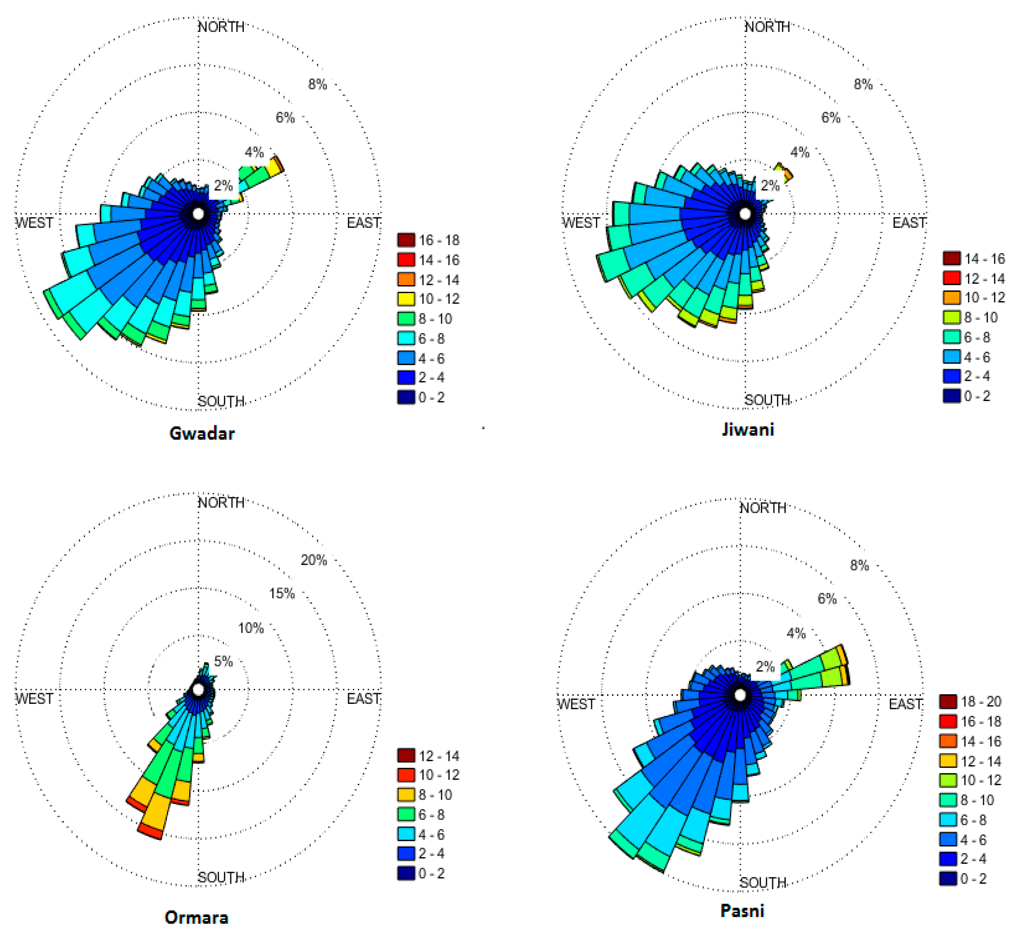
In this paper, coefficients of the WD function and WE characteristics were determined for the coastal areas of Pakistan (Gwadar, Jiwani, Ormara, and Pasni). Wind data from 2011 to 2016, measured at a 50 m height, were obtained from Karachi’s meteorological office. WE potentials were statistically evaluated for all regions based on hourly WS data. The actual WS data and different numerical methods were used to calculate WD parameters. Furthermore, the wind rose chart was used to visualize the WS patterns in all regions, as represented in Figure 2, which shows the wind density direction concerning all areas’ wind frequencies. The wind rose chart helps with the decision for wind design machines at any site. The dominant WS direction is south to the west for Gwadar, southeast to the west for the Jiwani region, southwest to the west for the Ormara region, and south to the southwest for Pasni, as depicted in Figure 2.

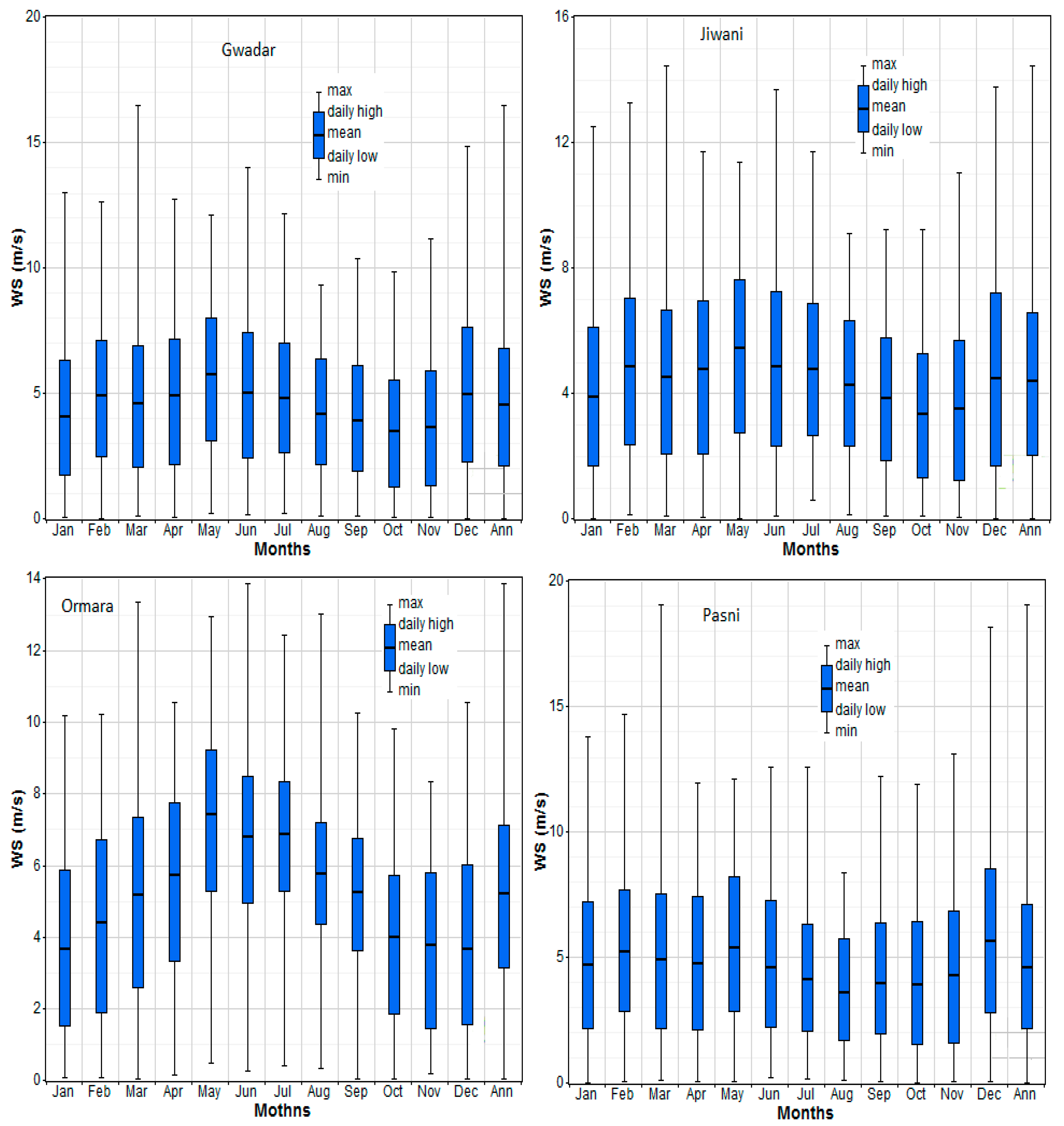
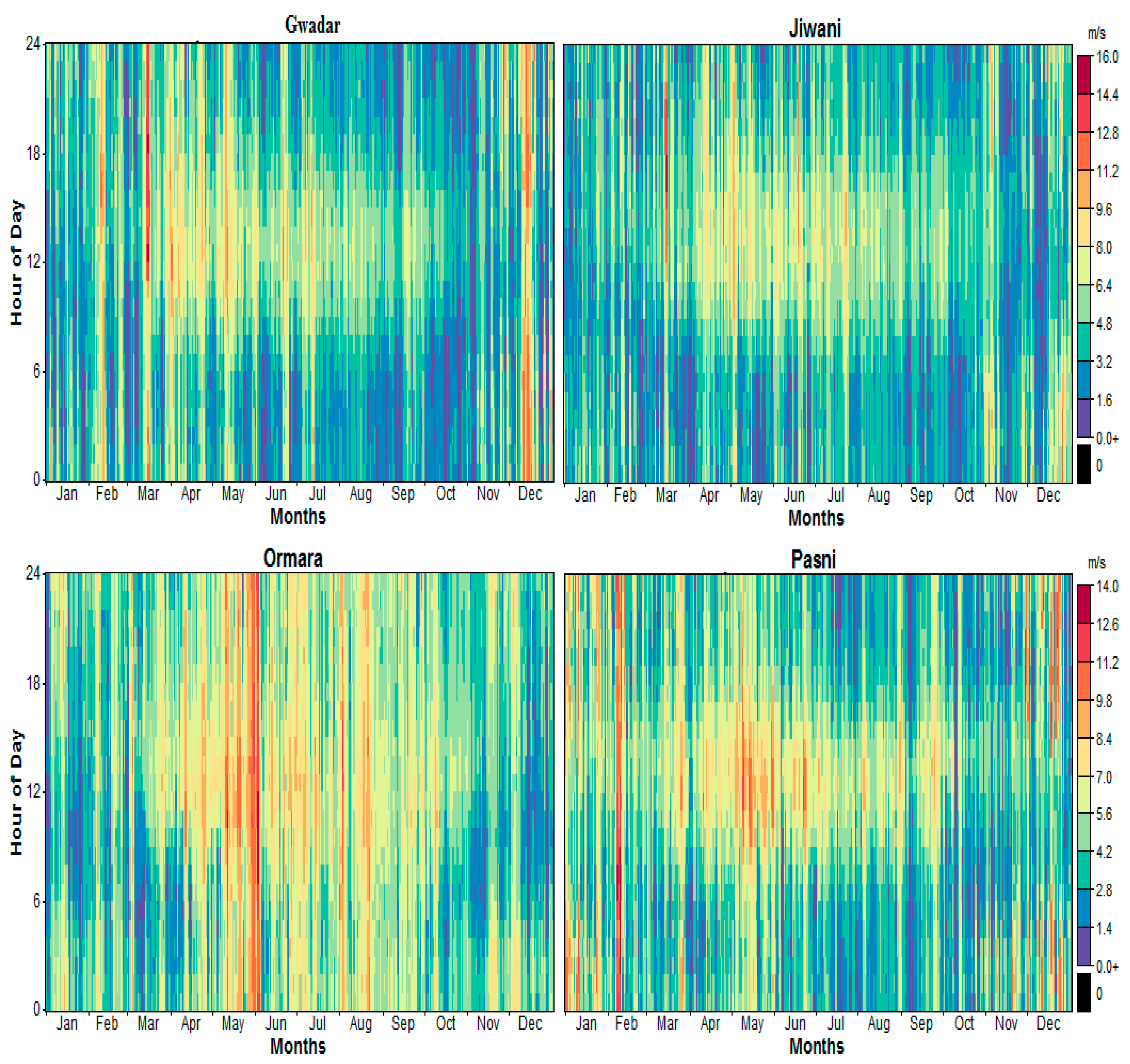
Hourly average WS data over six years for all four regions at 50 m height are shown in

Table 2. WS (m/s) statistics of all regions.

Regions	MWS	Minimum	Maximum	SD
Gwadar	4.579	0.299	10.642	2.088
Jiwani	4.423	0.263	10.212	1.990
Ormara	5.250	0.590	10.148	1.914
Pasni	4.652	0.244	11.241	2.199

. The maximum annual MWS of 5.25 m/s was detected at Ormara with an SD of 1.914 m/s, and the minimum MWS of 4.423 m/s was observed at Jiwani with an SD of 1.990 m/s. The data are arranged by monthly maximum and minimum, and daily low and high (in these months). The MWS, used to measure the seasonal variation in WS for all regions, is shown in Figure 3. According to Figure 3, the maximum monthly MWS was detected in May/Dec. Almost a minimum MWS was noticed in October in all regions. Moreover, years of representation of WS data are also shown in Figure 4 to visualize the WS statistic. It can be observed that the Ormara region is the windiest area compare to the others, while Jiwani is the least windy area.

4.2. Statistical Error Analysis (SEA)

The SEA is used to find the efficiency and best numerical method for each particular site. In this context, three statistical methods, such as RMSE, $R^2,$ and $X^2$ are used to calculate the efficiency and best method among eight numerical methods for each site. [31].

$$RMSE={\left(\frac{1}{N}{\displaystyle \sum }_{i=1}^N{\left(y_i-x_i\right)}^2\right)}^{\frac{1}{2}}$$

(26)

$$X^2=\frac{{{\displaystyle \sum }}_{i=1}^N{\left(y_i-x_i\right)}^2}{N-n}$$

(27)

$$R^2=\frac{{{\displaystyle \sum }}_{i=1}^N{\left(y_i-z\right)}^2-{{\displaystyle \sum }}_{i=1}^N{\left(y_i-x_i\right)}^2}{{{\displaystyle \sum }}_{i=1}^N{\left(y_i-z\right)}^2}$$

(28)

where N,$x_i,$z, n, and $y_i$ represent the number of observations, predicted data of WD, mean WS, number of constants used, and actual data, respectively. The aforementioned statistical error analysis is derived for eight numerical methods and gives rank to each numerical method to detect the best approach for each dataset. A detailed discussion follows in the coming section.

4.3. Analysis of the WD Function

The WD function is defined by the probability function f(v) corresponding with MWS. The WD functions for the six years 2011–2016 for the regions Gwadar, Jiwani, Ormara, and Pasni for eight numerical methods based on WSP and WCP are presented in Figure 5. The MWS and SD data for all regions are listed in

Table 3. Monthly WS and SD for all regions.

Months	Regions
	Gwadar		Jiwani		Ormara		Pasni
	WS	SD	WS	SD	WS	SD	WS	SD
	(m/s)	(m/s)	(m/s)	(m/s)	(m/s)	(m/s)	(m/s)	(m/s)
Jan	3.98	2.27	3.95	2.24	3.81	1.96	4.56	2.50
Feb	4.76	2.44	4.88	2.48	4.40	2.05	5.08	2.72
Mar	4.83	2.28	4.56	2.16	5.24	2.08	4.97	2.34
Apr	5.27	2.26	4.81	2.10	5.92	2.01	5.06	2.17
May	5.84	2.21	5.49	2.25	7.39	2.19	5.50	2.19
Jun	5.04	2.17	4.91	2.18	6.86	2.30	4.62	2.09
Jul	4.85	1.81	4.81	1.71	6.74	2.18	4.19	1.80
Aug	4.49	1.77	4.31	1.51	5.96	1.89	3.96	1.73
Sep	4.05	1.72	3.90	1.55	5.39	1.91	4.16	1.85
Oct	3.60	1.68	3.39	1.56	4.07	1.73	4.05	2.02
Nov	3.74	2.10	3.55	1.97	3.74	1.70	4.44	2.44
Dec	4.71	2.86	4.52	2.64	3.62	1.89	5.52	3.23

. Figure 5 verifies how the curves representing the WD function for each of the eight numerical methods included in this paper fit the histograms, giving an idea of which method offers the best fit to the data of collected WS. Furthermore, the statistical analysis results are listed in

Table 4. Weibull parameters and statistical analysis for Gwadar.

Numerical Methods	Weibull Parameters		Statistical Tests
	WSP	WCP	R2	RMSE	X2
Maximum likelihood	2.1350	5.1700	0.9620	0.0140	0.0213
Least squares	2.1440	5.1720	0.9577	0.0138	0.0229
WAsP	2.1070	5.1550	0.9501	0.0149	0.0258
Empirical method of Justus	2.1478	5.1426	0.9548	0.0143	0.0248
Energy pattern method	2.1300	5.1425	0.9522	0.0147	0.0255
Energy trend method	2.1710	5.0438	0.9454	0.0161	0.0261
Moment method	2.1365	5.1425	0.9532	0.0146	0.0255
Graphical method	2.0970	5.1510	0.9480	0.0151	0.0260

,

Table 5. Weibull parameters and statistical analysis for Jiwani.

Numerical Methods	Weibull Parameters		Statistical Tests
	WSP	WCP	R2	RMSE	X2
Maximum likelihood	2.174	4.993	0.9465	0.0161	0.0325
Least squares	2.160	5.003	0.9457	0.0162	0.0322
WAsP	2.156	4.983	0.9424	0.0167	0.0341
Empirical method of Justus	2.199	4.994	0.9502	0.0157	0.0317
Energy pattern method	2.182	4.994	0.9478	0.0160	0.0320
Energy trend method	2.072	4.844	0.9063	0.0213	0.0549
Moment method	2.188	4.994	0.9487	0.0159	0.0318
Graphical method	2.107	4.979	0.9336	0.0177	0.0357

,

Table 6. Weibull parameters and statistical analysis for Ormara.

Numerical Methods	Weibull Parameters		Statistical Tests
	WSP	WCP	R2	RMSE	X2
Maximum likelihood	2.354	5.915	0.9226	0.0177	0.0354
Least squares	2.178	5.973	0.9041	0.0182	0.0367
WAsP	2.496	5.978	0.9461	0.0153	0.0270
Empirical method of Justus	2.375	5.924	0.9266	0.0173	0.0350
Energy pattern method	2.392	5.923	0.9283	0.0172	0.0343
Energy trend method	2.188	4.726	0.8082	0.0284	0.0935
Moment method	2.366	5.924	0.9256	0.0174	0.0352
Graphical method	2.167	5.719	0.8506	0.0239	0.0675

and

Table 7. Weibull parameters and statistical analysis for Pasni.

Numerical Methods	Weibull Parameters		Statistical Tests
	WSP	WCP	R2	RMSE	X2
Maximum likelihood	2.053	5.255	0.9294	0.0173	0.0220
Least squares	2.163	5.236	0.9505	0.0151	0.0111
WAsP	1.918	5.166	0.8799	0.0220	0.0339
Empirical method of Justus	2.069	5.251	0.9328	0.0170	0.0216
Energy pattern method	2.016	5.250	0.9193	0.0183	0.0233
Energy trend method	1.863	4.822	0.8037	0.0297	0.0815
Moment method	2.057	5.251	0.9300	0.0173	0.0218
Graphical method	2.064	5.407	0.9446	0.0150	0.0202

. Finally,

Table 8. Ranking by statistical test results for eight numerical methods.

Numerical Methods	Regions				Discussion
	Gwadar	Jiwani	Ormara	Pasni
Maximum likelihood	1st	5th	5th	5th	-
Least squares	2nd	4th	6th	1st	-
WAsP	6th	6th	1st	7th	-
Empirical method of Justus	3rd	1st	3rd	3rd	1st choice
Energy pattern method	5th	3rd	2nd	6th	3rd choice
Energy trend method	8th	8th	8th	8th	-
Moment method	4th	2nd	4th	4th	2nd choice
Graphical method	7th	7th	7th	2nd	-

shows the ranking of all numerical methods for all regions.

4.4. Statistical Analysis of WSP and WCP

Statistical analyses are used to further explore the performance of these various procedures and their ability to match the measured results precisely. In this context, the statistical analysis results for a height of 50 m are listed in Table 4, Table 5, Table 6 and Table 7. According to the WSP, the observed value range for Gwadar was from 2.0970 to 2.1710, the WSP value range for Jiwani was 2.072 to 2.182, the WSP value range was from 2.188 to 2.496 for Ormara, and the WSP value varied from 1.863 to 2.069 for Pasni, all listed in Table 4, Table 5, Table 6 and Table 7. According to the above analysis, the Ormara region has greater constancy of WS than the other three regions, while the least constant region is Pasni compared to the other three regions. The value range of the WCP for all regions varied almost from 4 to 6, but the range for the Ormara region was 4.726 to 5.978, which means Ormara is windier than the other regions. Moreover, the theoretical results’ accuracies are listed in Table 4, Table 5, Table 6 and Table 7 for each site.

Furthermore, the ranking of eight numerical methods was calculated using statistical analysis results (RMSE, X², and R²). The numerical method is a good fit when the R² value is closer to unity while the X² value is closer to zero. According to these rules, eight numerical methods were ranked, as shown in Table 8. From Table 8, as we expected, it is impossible to say that one method is the best solution for all sites. From this analysis, for each dataset there is one preferred method, but this can be the worst for another dataset. The methodology used in this paper is necessary. For example, depicted in column 2, Table 8, the ML gave good results for the Gwadar region, while it did not give satisfactory results for the rest of the areas. Similarly, the EMJ gave the best outcome for the Jiwani region, but not the best for the other regions. Furthermore, the cumulative performance of each method for all regions is mentioned in the discussion column in Table 8. The EMJ and GM methods are the best and worst compromise, respectively, for all regions.

4.5. Evaluation of Power Density

The MWS and WPD were calculated for all coastal regions of Pakistan by using eight numerical methods to obtain WD parameters. The calculated results were compared with actual MWS and WPD values collected from measurements. We know that the difference between estimated WE and actual WE and the WD function data can be used to evaluate the accuracy of all eight numerical methods. The MWS $“V_m”$ and WPD $“P_m”$ for real-time data can be obtained using (29) and (30).

$$v_m=\frac{1}{n}{\displaystyle \sum }_{i=1}^n{v}_i$$

(29)

$$P_m=\frac{1}{2}\rho \overline{V^2}$$

(30)

The average of measured WS was 4.58 $\mathrm{m}/\mathrm{s}$, 4.42$\mathrm{m}/\mathrm{s}$, 5.27 $\mathrm{m}/\mathrm{s}$, and 4.67$\mathrm{m}/\mathrm{s}$ and the calculated power densities were 106 $\mathrm{w}/{\mathrm{m}}^2$, 93.7$\mathrm{w}/{\mathrm{m}}^2$, 145.7$\mathrm{w}/{\mathrm{m}}^2$, and 116.3 $\mathrm{w}/{\mathrm{m}}^2$, in Gwadar, Jiwani, Ormara, and Pasni, respectively. The results above were computed using real-time hourly WS from 2011 to 2016. According to this six-year period (2011–2016) of WS data, we analyzed that Ormara has a higher WE potential than the other three regions regarding the average WS and WPD. Furthermore, monthly and annual average WS and WPD for all regions are listed in

Table 9. Monthly and annual average WS and WPD for all regions.

Months	Regions
	Gwadar		Jiwani		Ormara		Pasni
	WS	WPD	WS	WPD	WS	WPD	WS	WPD
	m/s	w/m2	m/s	w/m2	m/s	w/m2	m/s	w/m2
Jan	3.98	82.50	3.95	79.20	3.81	63.00	4.56	118.40
Feb	4.76	123.90	4.88	131.20	4.40	87.40	5.08	160.90
Mar	4.83	119.70	4.56	101.40	5.24	130.10	4.97	133.40
Apr	5.27	140.00	4.81	108.10	5.92	170.10	5.06	124.30
May	5.84	173.80	5.49	152.10	7.39	310.70	5.50	151.30
Jun	5.04	124.70	4.91	118.20	6.86	263.70	4.62	99.40
Jul	4.85	100.10	4.81	95.10	6.74	246.60	4.19	71.50
Aug	4.49	83.30	4.31	67.40	5.96	169.50	3.96	61.20
Sep	4.05	63.30	3.90	54.00	5.39	131.60	4.16	72.00
Oct	3.60	48.40	3.39	40.20	4.07	64.20	4.05	74.00
Nov	3.74	67.70	3.55	40.20	3.74	52.90	4.44	109.30
Dec	4.71	145.00	4.52	122.10	3.62	52.90	5.52	222.00
Annual	4.68	106.00	4.42	93.70	5.27	145.70	4.67	116.30

to visualize the complete scenario, such as minimum and maximum WS and WPD in the six years. The maximum WS and WPD are observed in the summer session, while the minimum WS and WPD are observed in the winter session.

The help of WSP and WCP also obtained the average WS and WPD. The estimated average WS, $V_m,$ and WPD, $P_w,$ of the WD function can be calculated by using Equations (31) and (32) [27]:

$$V_w=c\mathrm{ᴦ}\left(1+\frac{1}{k}\right)$$

(31)

$$P_w=\frac{1}{2}\rho c^3\mathrm{ᴦ}\left(1+\frac{1}{k}\right)$$

(32)

Furthermore, the actual values were compared with estimated values to check for conformity. The WPD and MWS of eight numerical methods are listed in

Table 10. Average WS and WPD for eight numerical methods.

Numerical Methods	Regions
	Gwadar		Jiwani		Ormara		Pasni
	WS	WPD	WS	WPD	WS	WPD	WS	WPD
	m/s	w/m2	m/s	w/m2	m/s	w/m2	m/s	w/m2
Maximum likelihood	4.58	105.26	4.42	93.28	5.24	145.34	4.66	114.77
Least squares	4.50	104.98	4.43	94.38	5.29	159.43	4.64	108.06
WAsP	4.57	105.64	4.41	93.41	5.30	144.00	4.58	117.29
Empirical method of Justus	4.55	103.03	4.42	92.40	5.25	145.05	4.65	113.63
Energy pattern method	4.55	103.81	4.42	93.03	5.25	144.23	4.65	116.58
Energy trend method	4.47	96.27	4.29	89.08	4.19	78.65	4.28	98.72
Moment method	4.55	103.52	4.42	92.81	5.25	145.46	4.65	114.29
Graphical method	4.56	105.87	4.42	93.28	5.06	140.57	4.79	124.36

. In terms of calculated WPD based on the six-year data period examined, the EM, MLM, EPM, MM, LSRM, and WasPA algorithms showed optimum performance. At the same time, the ETM and GM provided weak performance for the whole period in four coastal regions of Pakistan.

5. Conclusions

This research presents the best numerical approach for determining the coefficients of the Weibull distribution function in four different coastal regions of Pakistan. All methods presented in this article were applied to monthly and yearly WS data for a period ranging between 2011 and 2016. The numerical results were analyzed by using three different types of statistical error tests, i.e., analysis of variance ($R^2$), chi-square ($X^2$) and RMSE. The suggested simulation model was proven appropriate for analyzing wind power generation capacity. It has been reported that it is critical to account for the monthly variations in wind speed using the Weibull approximation since wind energy potential varies greatly. According to the simulation findings, Ormara has the largest wind energy potential, whereas Jiwani is the area least possible for renewable energy. Statistical tests revealed that estimated values from all techniques, except for the ETM and GM, were close to actual data from all four sites. Future studies will consider more potential sites using the eight numerical methods.

References

1. Abdul, D.; Wenqi, J.; Tanveer, A. Prioritization of renewable energy source for electricity generation through AHP-VIKOR integrated methodology. Renew. Energy 2021, 184, 1018–1032. [Google Scholar] [CrossRef]
2. Asghar, R.; Ullah, Z.; Azeem, B.; Aslam, S.; Hashmi, M.H.; Rasool, E.; Shaker, B.; Anwar, M.J.; Mustafa, K. Wind Energy Potential in Pakistan: A Feasibility Study in Sindh Province. Energies 2022, 15, 8333. [Google Scholar] [CrossRef]
3. Azeem, B.; Ullah, Z.; Rehman, F.; Ali, S.M.; Haider, A.; Saeed, S.; Hussain, I.; Mehmood, C.; Khan, B. Levenberg-Marquardt SMC control of grid-tied Doubly Fed Induction Generator (DFIG) using FRT schemes under symmetrical fault. In Proceedings of the 1st International Conference on Power, Energy and Smart Grid (ICPESG), Mirpur Azad Kashmir, Pakistan, 9–10 April 2018; pp. 1–6. [Google Scholar] [CrossRef]
4. Ullah, K.; Basit, A.; Ullah, Z.; Asghar, R.; Aslam, S.; Yafoz, A. Line Overload Alleviations in Wind Energy Integrated Power Systems Using Automatic Generation Control. Sustainability 2022, 14, 11810. [Google Scholar] [CrossRef]
5. Usta, I.; Arik, I.; Yenilmez, I.; Kantar, Y.M. A new estimation approach based on moments for estimating Weibull parameters in wind power applications. Energy Convers. Manag. 2018, 164, 570–578. [Google Scholar] [CrossRef]
6. Hussain, I.; Ali, S.M.; Khan, B.; Ullah, Z.; Mehmood, C.A.; Jawad, M.; Farid, U.; Haider, A. Stochastic Wind Energy Management Model within smart grid framework: A joint bi-directional service level agreement (SLA) between Smart Grid and wind energy district prosumers. Renew. Energy 2019, 134, 1017–1033. [Google Scholar] [CrossRef]
7. Wei, J.; Zhang, Y.; Wang, J.; Wu, L.; Zhao, P.; Jiang, Z. Decentralized Demand Management Based on Alternating Direction Method of Multipliers Algorithm for Industrial Park with CHP Units and Thermal Storage. J. Mod. Power Syst. Clean Energy 2022, 10, 120–130. [Google Scholar] [CrossRef]
8. Saeed, S.; Asghar, R.; Mehmood, F.; Saleem, H.; Azeem, B.; Ullah, Z. Evaluating a Hybrid Circuit Topology for Fault-Ride through in DFIG-Based Wind Turbines. Sensors 2022, 22, 9314. [Google Scholar] [CrossRef]
9. Sahu, B.K. Wind energy developments and policies in China: A short review. Renew. Sustain. Energy Rev. 2018, 81, 1393–1405. [Google Scholar] [CrossRef]
10. Hernández-Escobedo, Q.; Perea-Moreno, A.-J.; Manzano-Agugliaro, F. Wind energy research in Mexico. Renew. Energy 2018, 123, 719–729. [Google Scholar] [CrossRef]
11. The Wind Power—Wind Energy Market Intelligence—Online Access > Countries > Pakistan. Available online: http://www.thewindpower.net/country_en_65_pakistan.php (accessed on 18 January 2023).
12. Kamran, M. Current status and future success of renewable energy in Pakistan. Renew. Sustain. Energy Rev. 2018, 82, 609–617. [Google Scholar] [CrossRef]
13. Baloch, M.; Abro, S.; Sarwar Kaloi, G.; Mirjat, N.; Tahir, S.; Nadeem, M.; Gul, M.; Memon, Z.; Kumar, M. A research on electricity generation from wind corridors of Pakistan (two provinces): A technical proposal for remote zones. Sustainability 2017, 9, 1611. [Google Scholar] [CrossRef]
14. Afanasyeva, S.; Saari, J.; Kalkofen, M.; Partanen, J.; Pyrhönen, O. Technical, economic and uncertainty modelling of a wind farm project. Energy Convers. Manag. 2016, 107, 22–33. [Google Scholar] [CrossRef]
15. Marini, M.; Russo, M. Effects of wind source uncertainties on investment cost analysis. In Proceedings of the International Conference on Wind Power for the 21st Century, Kassel, Germania, 25–27 September 2000; pp. 45–48. [Google Scholar]
16. Biswas, P.P.; Suganthan, P.N.; Amaratunga, G.A.J. Optimal power flow solutions incorporating stochastic .ind and solar power. Energy Convers. Manag. 2017, 148, 1194–1207. [Google Scholar] [CrossRef]
17. Garcia, A.; Torres, J.; Prieto, E.; Francisco, A.D. Fitting wind speed distributions: A case study. Sol. Energy 1998, 62, 139–144. [Google Scholar] [CrossRef]
18. Shi, H.; Dong, Z.; Xiao, N.; Huang, Q. Wind Speed Distributions Used in Wind Energy Assessment: A Review. Front. Energy Res. 2021, 9, 769920. [Google Scholar] [CrossRef]
19. Chang, T.P. Estimation of wind energy potential using different probability density functions. Appl. Energy 2011, 88, 1848–1856. [Google Scholar] [CrossRef]
20. Ozay, C.; Celiktas, M.S. Statistical analysis of wind speed using two-parameter Weibull distribution in Alaçatı region. Energy Convers. Manag. 2016, 121, 49–54. [Google Scholar] [CrossRef]
21. Kaplan, Y.A. Determination of the best Weibull methods for wind power assessment in the southern region of Turkey. IET Renew. Power Gener. 2016, 11, 175–182. [Google Scholar] [CrossRef]
22. Patidar, H.; Shende, V.; Baredar, P.; Soni, A. Comparative study of offshore wind energy potential assessment using different Weibull parameters estimation methods. Environ. Sci. Pollut. Res. 2022, 29, 46341–46356. [Google Scholar] [CrossRef]
23. Kaplan, Y.A.; Lam, R.P.; Lam, L.C.H.; Hoxey, R.P.; Robertson, A.P.; Richardson, G.M.; Cook, N. Calculation of Weibull distribution parameters at low wind speed and performance analysis. Proc. Inst. Civ. Eng.—Energy 2022, 175, 195–204. [Google Scholar] [CrossRef]
24. Kaplan, Y.A. Comparison of the Performance of the Methods Used to Find the Weibull Parameters at Different Heights. Arab. J. Sci. Eng. 2021, 46, 12145–12153. [Google Scholar] [CrossRef]
25. Kaplan, Y. Determination of Weibull parameters with using standard deviation method and performance comparison at different locations. Sci. Iran. 2019, 27, 3075–3083. [Google Scholar] [CrossRef]
26. Sumair, M.; Aized, T.; Bhutta, M.M.A.; Siddiqui, F.A.; Tehreem, L.; Chaudhry, A. Method of Four Moments Mixture-A new approach for parametric estimation of Weibull Probability Distribution for wind potential estimation applications. Renew. Energy 2022, 191, 291–304. [Google Scholar] [CrossRef]
27. Safari, M.A.M.; Masseran, N.; Majid, M.H.A. Wind energy potential assessment using Weibull distribution with various numerical estimation methods: A case study in Mersing and Port Dickson, Malaysia. Theor. Appl. Clim. 2022, 148, 1085–1110. [Google Scholar] [CrossRef]
28. Djiela, R.H.T.; Kapen, P.T.; Tchuen, G. Wind energy of Cameroon by determining Weibull parameters: Potential of a environmentally friendly energy. Int. J. Environ. Sci. Technol. 2020, 18, 2251–2270. [Google Scholar] [CrossRef]
29. Allouhi, A.; Zamzoum, O.; Islam, M.R.; Saidur, R.; Kousksou, T.; Jamil, A.; Derouich, A. Evaluation of wind energy potential in Morocco’s coastal regions. Renew. Sustain. Energy Rev. 2017, 72, 311–324. [Google Scholar] [CrossRef]
30. Signe, E.B.K.; Kanmogne, A.; Emmanuel, G.D.; Meva’A, L. Comparison of seven numerical methods for determining Weibull parameters of wind for sustainable energy in Douala, Cameroon. Int. J. Energy Sect. Manag. 2019, 13, 903–915. [Google Scholar] [CrossRef]
31. Chaurasiya, P.K.; Ahmed, S.; Warudkar, V. Comparative analysis of Weibull parameters for wind data measured from met-mast and remote sensing techniques. Renew. Energy 2018, 115, 1153–1165. [Google Scholar] [CrossRef]
32. Teimourian, H.; Abubakar, M.; Yildiz, M.; Teimourian, A. A Comparative Study on Wind Energy Assessment Distribution Models: A Case Study on Weibull Distribution. Energies 2022, 15, 5684. [Google Scholar] [CrossRef]
33. Bingöl, F. Comparison of Weibull Estimation Methods for Diverse Winds. Adv. Meteorol. 2020, 2020, 3638423. [Google Scholar] [CrossRef]
34. Bagiorgas, H.S.; Mihalakakou, G.; Rehman, S.; Al-Hadhrami, L.M. Wind power potential assessment for seven buoys data collection stations in Aegean Sea using Weibull distribution function. J. Renew. Sustain. Energy 2012, 4, 013119. [Google Scholar] [CrossRef]
35. Saeed, M.K.; Salam, A.; Rehman, A.U. Comparison of six different methods of Weibull distribution for wind power assessment: A case study for a site in the Northern region of Pakistan. Sustain. Energy Technol. Assessments 2019, 36, 100541. [Google Scholar] [CrossRef]
36. Aries, N.; Boudia, S.M.; Ounis, H. Deep assessment of wind speed distribution models: A case study of four sites in Algeria. Energy Convers. Manag. 2018, 155, 78–90. [Google Scholar] [CrossRef]
37. Baseer, M.A.; Meyer, J.P.; Rehman, S.; Alam, M.M. Wind power characteristics of seven data collection sites in Jubail, Saudi Arabia using Weibull parameters. Renew. Energy 2017, 102, 35–49. [Google Scholar] [CrossRef] [Green Version]
38. UL Solutions. Windographer: Wind Data Analytics and Visualization Solution. Available online: https://www.ul.com/services/windographer-wind-data-analytics-and-visualization-solution (accessed on 19 January 2023).
Figure 1. Proposed wind energy sites in Pakistan [13].
Energies 16 01515 g001
Figure 2. Wind rose plots for all regions.
Energies 16 01515 g002
Figure 3. Daily high, low, MWS, and monthly maximum and minimum wind speeds in all regions [38].
Energies 16 01515 g003
Figure 4. Monthly and daily representation of WS data from all regions [34].
Energies 16 01515 g004
Figure 5. WD functions for all regions.
Energies 16 01515 g005