Highlights
What are the main findings?
- Energy consumption reduction up to 24% with the use of ECMS algorithm
- Method for EMS algorithms comparison under the same required energy
- Back engineering extracted commercial algorithm based on experimental data
What is the implication of the main finding?
- ECMS adaptability advantage can be utilized under different driving conditions
Abstract
The study examines alternative on-board energy management system (EMS) supervisory control algorithms for plug-in hybrid electric vehicles. The optimum fuel consumption was sought between an equivalent consumption minimization strategy (ECMS) algorithm and a back-engineered commercial rule-based (RB) one, under different operating conditions. The RB algorithm was first validated with experimental data. A method to assess different algorithms under identical states of charge variations, vehicle distance travelled, and wheel power demand criteria is first demonstrated. Implementing this method to evaluate the two algorithms leads to fuel consumption corrections of up to 8%, compared to applying no correction. We argue that such a correction should always be used in relevant studies. Overall, results show that the ECMS algorithm leads to lower fuel consumption than the RB one in most driving conditions. The difference maximizes at low average speeds (<40 km/h), where the RB leads to more frequent low load engine operation. The two algorithms lead to fuel consumption differences of 3.4% over the WLTC, while the maximum difference of 24.2% was observed for a driving cycle with low average speed (18.4 km/h). Further to fuel consumption performance optimization, the ECMS algorithm also appears superior in terms of adaptability to different driving cycles.
1. Introduction
Global warming due to increasing emissions of greenhouse gases (GHG) appears today as the main environmental pressure [1]. Transport is one of the key sources of manmade carbon dioxide (CO2) emissions [1,2,3]. This has led authorities around the world to set targets and take measures to reduce these emissions [3,4]. The European Union (EU) has set a target of reducing CO2 levels from new passenger cars by 37.5% by 2030, compared to 2021 [5]. Therefore, solutions such as electrified vehicles are promoted by the automotive industry to meet these targets [6].
Hybrid Electric Vehicles (HEVs) and Plug-in Hybrid Electric Vehicles (PHEVs) are currently the most widespread options for electrified vehicles in the market. HEVs and PHEVs have two independent energy sources, namely the battery and the fuel tank. However, only PHEVs can be charged directly by grid power and can cover substantial ranges (e.g., the latest models appear to have an electrical range of 100 km or 65 miles [7]) with electric power alone [6]. The share and mix between battery and engine power are constantly being decided during operation by an on-board energy management system (EMS) [1,6,8,9]. The EMS performance has a significant impact on fuel consumption (FC), which is directly linked to CO2 emissions. Therefore, EMS supervisory algorithms can be optimized to further decrease CO2 emissions from PHEVs.
Wu et al. [10] showed that there are a variety of principles for EMS algorithms. The main categories can be distinguished into rule-based (RB), optimization-based (OB), and learning-based (LB) ones. RB algorithms rely on a fixed set of rules, without a priori knowledge of driving conditions. OB algorithms are further split to offline or online ones. In online OB algorithms, such as the Equivalent Consumption Minimization Strategy (ECMS) [10,11,12,13], an instantaneous optimization is conducted based on current vehicle operation. In offline OB algorithms, a cost function is optimized for the complete driving cycle. Dynamic Programming (DP) [14,15] and Pontryagin’s Minimum Principle (PMP) [10,16] are some of the common offline OB algorithms. LB algorithms are capable of instantaneously and in real time controlling and learning the optimal power split operations. Reinforcement Learning [17,18] and Artificial Neural Networks are some principles that are used in LB algorithms implementation [10].
There are only limited works in the literature on how different algorithm categories compare to each other under different operation conditions. Actually, Torreglosa et al. [19] mentioned that the optimization algorithms presented in the literature are seldom compared against commercial RB strategies. In their study, they compared different EMSs for HEVs with RB strategies using FASTSim, an open-source tool that includes validated HEV RB models. That analysis showed that optimum EMSs may provide fuel consumption benefits of 5% to 10%, compared to commercial RB EMSs. Wu et al. [20] proposed an optimization-based strategy that appeared to reduce the fuel consumption of a 2010 Toyota Prius hybrid by 3.5–6%, compared to an RB algorithm that was earlier published by Kim et al. [21]. Hwang et al. [22] applied particle swarm optimization to improve the fuel economy of a power split hybrid, and showed up to 9.4% improvement compared to an RB algorithm. This limited previous work showed that there are further margins to improve fuel consumption over commercially applied algorithms.
In assessing the performance of different algorithms, one needs to make sure that the exact operation profile is followed over computer simulations or real-world experimentation with the various EMS approaches. Fuel consumption differences of only a few percentage units, such as those expected when varying the EMS, can be observed only due to slight deviations of the original speed profile in consecutive simulations, e.g., due to underpowering accelerations. Moreover, it needs to be ensured that fuel consumption improvement is assessed under the same state of charge levels (SOC) to avoid part of the difference only being due to variation in the battery depletion levels, e.g., over consecutive simulations. Although such conditions may be self-evident, these are seldom if at all demonstrated in published EMS algorithm comparison studies.
The article focuses on the comparative assessment of commercial RB and ECMS based algorithms for a plug-in hybrid vehicle powertrain. The purpose is to examine if further FC reduction can be achieved by introducing an enhanced EMS over a commercial one. A method is first presented to compare fuel consumption over identical battery state of charge (SOC) levels, vehicle distance traveled and wheel power demand. The proposed method suggests novel corrections for the fuel energy consumption of the compared EMS algorithms. More specifically, the method introduces correction terms for the deviations in the final SOC values, propulsion energy and benefits from regenerative braking between the compared EMS algorithms. We propose that such a method needs to be used in all similar studies of fuel consumption comparison.
2. Methods
2.1. Back-Engineered EMS Algorithm
A vehicle simulator of a parallel P2 PHEV [23] has been built in the AVL Cruise simulation platform. Its overall performance has been validated with actual experimental data collected by tests on an actual vehicle in the chassis dynamometer of Aristotle University. The vehicle’s technical specifications are listed in Table 1.

Table 1.
Parallel P2 PHEV Technical Specifications.
Table 2 shows the tests conducted in the lab on the particular vehicle to understand the performance of its stock EMS algorithm. A Worldwide harmonized Light vehicles Test Cycle (WLTC) [24] and an ERMES cycle [25] have been used for the tests. The different cycles are distinguished into cold and hot start ones, depending on whether the start engine coolant temperature was lower than 35 °C or higher than 70 °C, respectively. A single case with intermediate start temperature is identified as warm start in Table 2.
Table 2.
Driving cycles and specifications use for experimental validation of the back-engineered algorithm.
These experiments have been used to back-engineer the rules of the heuristic controller on-board the commercial vehicle. In this paper, the RB algorithm is a specialization of the general methodology described by Doulgeris et al. [26], while the specific controller algorithm is described in detail by Doulgeris et al. [27].
Figure 1 shows the flowchart of the RB algorithm. The engine switches on if the power demand, vehicle speed or acceleration, and SOC level are above specific thresholds. The power demand threshold for engine start depends on the SOC level. The engine always shuts off when the power demand becomes negative.

Figure 1.
Stock rule-based algorithm extracted from experimental evidence.
Figure 2 shows the engine power output decided by the algorithm curve, depending on the gear engaged (x-axis) and the vehicle speed (parameter). If the engine meets the criteria for switch-on according to Figure 1, then the engine power output is determined by Figure 2 depending on current vehicle speed and gear.

Figure 2.
Engine power output decided by the RB algorithm depending on gear and vehicle speed.
2.2. Alternative Algorithm Description
An Equivalent Consumption Minimization Strategy (ECMS) algorithm has been developed in the current study, as an alternative to the back-engineered RB one. Both of the algorithms—ECMS and the back-engineered one—are applied to the same vehicle simulator platform of parallel P2 PHEV that has been built in the AVL Cruise simulator platform. The ECMS algorithm aims at optimizing a predefined FC cost function for given operation conditions. The general cost function for fuel consumption optimization of a hybrid vehicle is given in Equation (1), where is a performance index that needs to be minimized. The integral term represents the total fuel consumption over a complete driving profile, as it integrates the instantaneous FC from an initial () to a terminal time stamp (). FC depends on the normalized engine load function u that ranges between 0 (engine shut off) to 1 (operation at full power—), according to Equation (2). The first term in Equation (1) is used as a soft constraint for the value of the SOC at the end of the cycle (). With the use of the function, SOC deviations from the final target value () are being penalized. The choice of the value depends on the examined study. Usually, in PHEVs applications, the charge depletion is permitted because the battery can be charged from the electric power grid. As a result, for PHEVs applications, the can be lower than the initial value of SOC [8,9].
The optimization of Equation (1) leads to the determination of the u for every second of the driving cycle, which in turn gives the instantaneous engine power output by means of Equation (2).
The ECMS optimization is subject to the conditions of the set of Equations (3)–(6). Equation (3) presents the power balance for the powertrain of a P2 parallel hybrid vehicle [28]. The sum of the demanded power at wheels () and the mechanical power losses () must be equal to the mechanical power output from the main power units (electric motor power— and engine power—). If the vehicle velocity is known, then the and can be determined by a vehicle power-based model. We have set up a vehicle model in AVL Cruise for this purpose. So, with the use of Equation (3), the power output of the electric motor is determined.
Equations (4)–(6) correspond to the physical constraints of the powertrain components. Equation (4) suggests that the engine cannot overcome its full load curve, represented by the maximum engine power output (). The electric motor is also limited by its full load curve, depending on whether it works as a motor ( > 0) or generator ( < 0) (Equation (5)), with corresponding limits given by and . Finally, the battery SOC cannot exceed a range of maximum () and minimum () levels for the purpose of maintaining battery life (Equation (6)).
Optimizing Equation (1) within the set of Conditions (3)–(6) is only possible when the operation mission is known a priori. In the real-world, a priori knowledge of the driving profile application is known only over in-lab tests and not for on-road driving. For on-road operation, the ECMS will have to be locally optimized according to the present driving conditions. Such local optimization is achieved by means of Equation (7), where the integral term of Equation (1) has been eliminated. In Equation (7), the engine fuel rate and the battery power flow expressed in terms of an equivalent fuel rate (Equation (8)—where QLHV is the fuel’s lower heating value) result in an equivalent total fuel mass rate by means of the equivalence factor (Equation (9)). The latter comprises the constant term and a penalization term that depends on SOC. The term is used as the main weighting factor of the inside the cost function. The p penalizes deviations of the current SOC values from the target. The usage of the p term is similar to the one of the term in Equation (1). The difference is that the penalization is made for the instantaneous values of SOC instead of the SOC value at the end of the cycle, because the optimization is only carried out locally. The battery power () in Equation (8) can be positive for power outflux from the battery (Equation (10a)) and negative when the EM acts as a generator that charges the battery (Equation (10b)), with and being the battery and electric motor efficiencies, respectively.
The algorithm basically decides on the engine operation variable u(t) in Equation (2) that leads to the lowest total equivalent fuel mass (). This procedure is repeated in every second of the complete mission profile. The algorithm takes into account two conditions regarding the potential battery charge or discharge. The first one is that a potential battery charge will lead to an SOC surplus, which can be utilized in the future. The second condition is that a present battery discharge generates a requirement for a future battery charge in order to retain the battery SOC within certain limits. An optimal solution can be guaranteed if the s term in Equation (7) is adapted appropriately (Equation (9)). In this way, although the s-by-s optimization cannot achieve as good a performance as the global optimal solution, it still produces a practical optimization solution that can be integrated in EMS without knowledge of the forthcoming driving profile.
Three alternative expressions for p have been examined in the current work (Equations (11a)–(11c)). In Type A expression, p is proportional to the difference of current SOC over a constant reference value (Equation (12a)). Therefore, this expression tries to keep SOC at a value close to the reference one over the complete driving profile—and it is tuned by a proportional term (). In Type B, the value varies with travelled distance (Equation (12b) [29]). The algorithm also tries to keep the current SOC close to the value, as in Type A. More specifically, in Type B, the value starts with an initial value () and then the decreases proportionally with the until it reaches the target SOC value (). In Type B, the total driving distance () must be either known or estimated. Some research articles mention that this type of linear SOC trajectory with distance seems to be close to the global optimal solution [30,31]. In Type C expression, a specific SOC window is used for determining p [8] (Equation (11c)). More specifically, the p value dependents on SOC, a target value for the SOC (, selected maximum and minimum SOC values and a selected superscript for the penalization function (). With this expression, SOC is retained above a certain level in order to ensure the battery physical constraints () proactively with the adaptation of the equivalence factor. Moreover, this expression constrains battery charging during charge sustain operation until a rational level (e.g., ).
Attention is required in selecting the parameters for each expression to achieve feasible solutions. For example, in our effort for parameters tuning, we spotted that some parameter combinations led to extremely low SOC levels or even that the vehicle could not follow the speed profile. So, after a trial-and-error basis in order to achieve feasible solutions, the setup of the algorithm parameters is presented in Table 3.
Table 3.
Parameters selected for the three ECMS versions.
The ECMS algorithm flowchart is illustrated in Figure 3. ECMS requires power demand, vehicle velocity, gear number and current SOC as input data. The first step is to select the numerical values for the physical limitations according Equations (4)–(6). After that, the algorithm calculates the equivalent fuel rate for the different candidate operating points by adjusting the equivalent consumption of the electrical motor according to the SOC, as described in Equations (9) and (11a)–(12b). Finally, the algorithm selects the case with the minimum fuel mass, which is then translated into specific torque outputs of the ICE and the electric motor.

Figure 3.
ECMS Procedure Overview.
2.3. Corrections for the Assessment of Different Algorithms
The assessment of different EMS algorithms needs to be carried out on a fair basis. Each EMS algorithm leads to different decisions for engine and motor engagement (Equation (2)) that may slightly affect the speed of the vehicle due to power availability and gear change interference. The different speed profiles will, in turn, result in a slightly different demanded power profile for each algorithm. These differences could have been avoided by backward modeling, because this approach guarantees that the vehicle exactly follows the target speed. However, in our approach, the forward modeling is chosen because forward simulators are based on physical causality. With these simulators, online control strategies can be developed [8]. Moreover, the SOC difference between trip start and end may differ between various algorithms. Nevertheless, when assessing the impacts of different algorithms on FC, one needs to make sure that the distance, demanded energy, and SOC differences are identical in the various simulations.
A method to adjust for such potential differences is, therefore, introduced. Assuming a total energy consumption over a theoretical accurate driving profile in each simulation, variations of this profile will lead to energy differences, not because of EMS performance but because of distance and SOC variations in each simulation. A corrected fuel-equivalent energy consumption (CE) can, therefore, be estimated from the simulated one (SE) by correcting for deviations in the SOC (), propulsion energy () and contribution of regenerative braking () in Equation (13). correction is needed to make sure that all simulations result in identical final SOC. The term corrects for slight differences in the driving profile (speed, acceleration and distance) of the simulations of a given driving sequence. Finally, adjusts the energy consumption when the simulated regenerative braking energy benefits are different from the ones calculated in the theoretically accurate driving profile. In that way, the energy differences due to driving profile variations at the braking phases can be corrected. The corrected energy correction of Equation (13) should be implemented in all relevant works where different optimization algorithms are being compared.
Equation (14) describes as the fuel energy delivery that covers the difference between the simulated and reference depleted energies from the battery (). In the denominator of Equation (14), the average product of the individual components’ efficiencies has been considered for the time moments that the battery is charged from the ICE, with being the ICE efficiency. The calculation for the reference value of the depleted battery energy is presented in Equation (15). The value is calculated as a difference from a final SOC level, which in our case has been selected to be 14%, with and being the battery capacity and average battery voltage, respectively.
The —Equation (16)—is the fuel energy that should be supplied to equalize the simulated energy demand at gearbox () with the one calculated from the theoretical speed profile (). The ICE efficiency should be the average one during positive power demand at gearbox inlet (). —Equation (17)—is the energy demand for vehicle motion for positive tractive force at the wheels (), with and being the force, theoretical vehicle speed and average transmission efficiency from gearbox inlet to vehicle wheels, respectively. consists of a polynomial function of vehicle speed (which corresponds to road loads) and the term for vehicle acceleration (Equation (18)—, , are coast down test coefficients and is the vehicle mass).
ΔEREG—Equation (19)—expresses the potential fuel energy that can be saved if the simulated speed profile was identical to the theoretical one () during decelerations. The simulated battery energy influx is calculated for the time instances that the power demand at gearbox inlet is negative. To convert the battery energy influx difference to fuel energy, the same average product of efficiencies as the one in Equation (14) has been used. The —Equation (20)—is the potential energy of braking that can be recuperated. In this calculation, the negative energy influx from the wheels () is calculated based on Equation (21). In the current study, the share of the total braking energy that can be recuperated () is assumed to be 40% of the total braking energy, while the rest is consumed at the mechanical brakes. The losses from the gearbox inlet up to the battery have been taken into account by the average product of the EM and battery efficiencies during the time events that is negative.
2.4. Drive Cycles Used in the Simulations
The performance of the Rule Based (RB) and the different types of ECMS Based (EB) algorithms are compared in different driving cycles, according to Table 4. Firstly, they are compared in WLTC driving cycle. After that, various driving cycles have been used in order to examine different conditions and identify the best algorithm in each case. For WLTC, ERMES and 10-15 Mode [32] cycles, the individual segments have been examined as well. Table 4 displays a summary of the characteristics of the different driving cycles that have been used. All simulations have been conducted with the same initial SOC of 20%, which allows a comparison of the algorithms during the most challenging charge sustain mode.
Table 4.
Simulated Driving Cycles and characteristics.
3. Results
3.1. Validation of the Rule Based Algorithm
Figure 4 and Figure 5 present examples for model accuracy in SOC and fuel consumption, respectively, for four of the seven conducted tests (Table 2). The initial SOC was the actual one at the beginning of each test. The simulated SOC profile satisfactorily follows the measured one during the course of each cycle. This can be reflected by the high correlation coefficient values for SOC (), which are higher than 69%. There is only one exception, for WLTC CS HOT1, where our back-engineered RB results in higher battery depletion in the 1000–1200 s range compared to the measured one. Apart from this, the simulated SOC follows the measured trend with a rather constant offset.

Figure 4.
SOC measurement vs. simulation—examples.
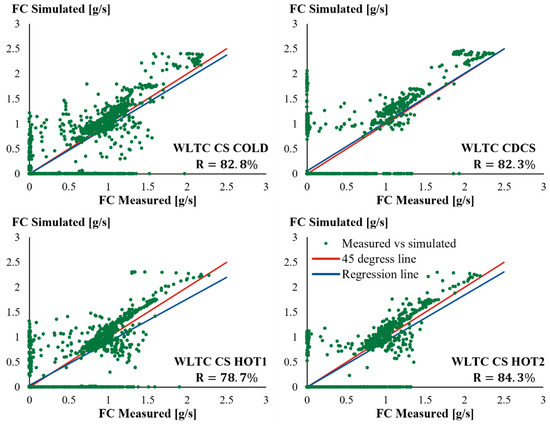
Figure 5.
FC measurement vs. simulation—examples.
Table 5 compares the total simulated and measured FC and final SOC () values for the seven tests conducted. The absolute error in the simulation of total FC is lower than 7% for five of the seven tests. In the WLTC CD and WLTC CDCS tests, the FC estimation error is higher, but over very low FC values that overall lead to satisfactory deviations (WLTC CD: 0.5 g/km; WLTC CDCS: 4.2 g/km). The correlation coefficient between instantaneous measured and simulated fuel consumption () is always higher than 70% except in WLTC CD (57.7%). In WLTC CD, the initial SOC is rather high (71.4%) so the engine engagement is limited leading to few points where the instantaneous fuel consumption is non-zero, and this leads to a drop of the regression coefficient. With regard to battery SOC, the simulated final SOC values are quite close to the measured ones for WLTC. For the ERMES cases, the simulated SOC varies more than the measured one in WLTC. Additionally, for the ERMES CS the value is negative. This means that the simulated battery charging events do not follow the measured ones for that test. It is worth mentioning that the parameters tuning for engine start/shut-down events (Figure 1) were based on the WLTC tests experimental data. As the ERMES cycle has different characteristics, we expected that the model could not have the same accuracy as in the WLTC tests. For all the other test cases, the is higher than 69% which implies satisfactory model performance.
Table 5.
Total FC and ΔSOC Comparison.
3.2. Comparative Assessment of RB and EB Algorithms in WLTC
Table 6 summarizes the simulation results for the three ECMS types (EBA, EBB, EBC) and the RB algorithm over WLTC. The FC values show correspondence to the simulation output (SFC) and the corrected ones (CFC), according to Equations (13)–(21). The table values clearly show that if no correction was introduced then one would come up with totally wrong conclusions regarding the relative performance of the different algorithms. For example, EBC leads to the highest FC difference over the RB (−3.4%), which is actually lower than the magnitude of the correction (−5.6%). Had the correction not been applied, the EBC would have actually resulted in +4.9% higher FC than the RB, i.e., this would have led to an entirely opposite conclusion than what is actually reached using the corrected values. This can be explained because the ΔESOC correction turns out negative for the EB and positive for the RB cases. The negative value for ΔESOC means that the final SOC is higher compared to the reference one in EB, and vice versa for RB. Additionally, Table 6 shows that ΔEPRO has a higher impact on EB cases. This indicates that the simulated speed profile in the RB simulation better follows the theoretical one than in EB simulations.
Table 6.
Consumption and mean efficiency values of the main powertrain components for WLTC.
The net energy flows between the different powertrain components during WLTC are presented in Figure 6. The shown energy flows stand for the positive propulsion instances. The electrical energy from the battery (2.89 MJ) and the energy demand at the gearbox inlet (13.2 MJ) have been adjusted to the exact same values in order to ensure that the comparison of the different algorithms is on a fair basis. Furthermore, the shown fuel energy consumption is the corrected one, which has been calculated from Equation (13).

Figure 6.
Net energy flows (kJ) for positive propulsion instances in WLTC for ECMS-Based Type A (EBA) algorithm, ECMS-Based Type B (EBB) algorithm, ECMS-Based Type C (EBC) algorithm and Rule-Based (RB) algorithm. ICE: Internal Combustion Engine, EM: Electric Motor, B: Battery and GB: Gearbox, FT: Fuel tank. Negative numbers correspond to energy loss.
The electric motor may function either as a propulsion device or as a generator for battery charging, depending on power flux direction. Assuming positive power flux from the battery to the gearbox, the energy flow through the EM ranges from 2121 kJ with the EBB to 1622 kJ with the RB algorithm. The difference in net energy flows is explained by the decisions of the different algorithms.
The lowest net EM energy flow is balanced by the maximum total energy outflux from the FT (30.6 MJ) with RB compared to EB. The simulation results in Table 6 show that the average ICE efficiency is quite close for all cases. Additionally, the demanded mechanical output energy from the ICE is higher in the RB case (11.59 MJ) compared to the EB (11.1–11.2 MJ). In RB, the electric motor contributes more for propulsion compared to the EB cases and results in higher battery discharge. This requires higher power demand from the ICE during hybrid mode to recharge the battery. That higher power demand for battery charging could have been saved had the EMS controller decided to directly command ICE propulsion with the assistance of the electric motor.
The above analysis showed that the description of the energy flows is very useful in order to understand the FC differences between RB and ECMS algorithms. For analysis convenience, in this paper a quantifiable metric for energy flow comparisons has been used, namely the average propulsion efficiency (). The is defined as the ratio of the demanded energy at the gearbox () over the sum of the two net energy flows from the energy sources during the positive propulsion phase (Equation (22)). The provided fuel energy is the corrected one, but only during the propulsion phases. Therefore, the correction terms of and have been added to the simulated fuel energy. Additionally, the reference battery depleted energy has been considered in the denominator. Table 6 shows that the RB algorithm results in the lowest propulsion efficiency and that leads to the highest fuel consumption.
As a benchmark, the results of Table 6 that have been obtained with localized optimization are compared to the global optimum for the known profile of WLTC. To do so, we have properly parameterized the hybrid electric vehicle model of Sundstrom et al. [34], which uses a DP a solution as an EMS algorithm. The parameterization has been achieved using exactly the same values for the individual components (ICE, EM, battery, Gearbox, axles, vehicle resistances and weight) with the ones used in the AVL Cruise simulated model. The DP model delivered 640.9 g as global optimum CFC, which is 7.3% lower than the one from the best-performing EBC (640.9 g vs. 691.4 g).
3.3. Comparison of RB and EB Algorithms for Other Cycles
Figure 7 illustrates the relative CFC difference between EB and RB algorithms for the different cycles. In most cases, EB achieves lower fuel consumption compared to RB. The highest FC reduction is observed for WLTC Low, which is 22.1–24.2% depending on the EB type, while the highest EB increase over RB is 2.7% over the ERMES Extra Urban. EB outperforms RB in all cycles of low speed. Evidently, the restrictions of RB on engine switch on criteria (Figure 1) and power output (Figure 2) have a cost on FC reached, while the adaptability of ECMS (Figure 3) allows for a much better result to be obtained.

Figure 7.
Fuel consumption change in ECMS algorithm types vs. Rule Based algorithm case for different cycles. EBA: ECMS Based Type A, EBB: ECMS Based Type B, EBC: ECMS Based Type C.
Table 7 better explains how EBC and RB perform for a low speed (WLTC Low) and a high speed (ERMES Extra Urban) cycle. In WLTC Low, EBC results in a higher propulsion efficiency by eight percentage units compared to the RB, and this leads to 22% FC reduction (RB: 582 g and EBC: 453 g). The improvement in propulsion is mainly linked to the mean ICE efficiency in this case. As Figure 2 shows, RB selects to operate the engine at lower load for vehicle speeds 0–30 km/h, which results in low engine efficiency. In reality, this selection may have to do with the need to retain low noise, vibration and harshness (NVH) levels in the vehicle cabin during low-speed driving. On the other hand, ECMS algorithm decisions for the engine load are dependent on the optimization of a cost function—Equation (7). As a result of its optimization-based functionality, ECMS leads to higher ICE Mean efficiency by 3.7 percentage units compared to RB in WLTC Low.
Table 7.
Consumption and mean efficiency values of the main powertrain components for WLTC Low and ERMES Extra Urban in the case of Rule Based (RB) and ECMS Based—C (EBC) algorithms.
The FC with ECMS appears higher than RB only in the ERMES cycle, and in particular in ERMES Extra Urban. In order to explain this, we can look the propulsion efficiency values at Table 7. The RB algorithm has a higher propulsion efficiency by 0.6 percentage units compared to EBC. The ERMES has a much higher power requirement and stronger accelerations than WLTC, which was used to tune the parameters of the ECMS algorithm (Equations (11a)–(12b) and Table 3). A better tuning for high power cycles could lead to lower FC compared to RB.
4. Discussion and Conclusions
This study makes an assessment and performance analysis for two types of energy management algorithms, including a back-engineered stock RB algorithm and an ECMS one.
A novel methodology to assess the different algorithms on a fair basis has been developed, introducing corrections for distance travelled, final SOC level and energy propulsion differences between alternative simulations. Our analysis showed that the impact of such corrections on fuel consumption can exceed 5%. Hou et al. [35] also considered SOC corrections when comparing different EMS algorithms, and found the impact of these corrections to be no more than 1% in fuel consumption. However, they did not correct for propulsion energy demand and regenerative braking. Our analysis shows that all three corrections can have a measurable result on fuel consumption values when different EMS algorithms are compared, and these should not be neglected in relevant studies.
The energy flow analysis also showed that the EMS affects both the efficiency of each powertrain component and the net energy flow between components. Therefore, it is the combination of these two magnitudes that affects overall total fuel consumption. As a result, the efficiencies of the individual components can be quite close for the two different EMS algorithms, but the FC can differ for the same energy demand.
Another important finding is that different driving conditions affect the magnitude of FC reduction that can be achieved with an alternative algorithm. Regarding the WLTC cycle, it has been found that the potential FC reduction with the use of ECMS algorithm is 3.4% over RB. For benchmarking purposes, a DP global optimization algorithm has been used for comparison. This requires a priori knowledge of the driving profile to find the optimum solution. The DP led to a 7.3% lower FC compared to the one from ECMS. Sun et al. [13] demonstrated that, on average, the FC achieved with DP can be 6.7% lower compared to an ECMS algorithm. ECMS algorithms, therefore, seem to offer good adaptability to driving conditions and sufficiently good final fuel consumption, which is not very distant from the global optimum.
With the use of ECMS, we found that fuel consumption in driving cycles with low average speeds (lower than 20 km/h) can be improved by up to 24.2% compared to a stock RB algorithm. The magnitude of improvement achieved was actually similar to the ones reported by Geng et al. [36], who proposed a combination of DP and ECMS to reduce FC by up to 19.9% in NEDC compared to RB. In another study, Hao et al. [37] used an adaptive ECMS to decrease the FC by 8–15% compared to an RB algorithm on a mild parallel hybrid vehicle. In our case, this large difference was partly because the RB forced the engine to operate at low loads when switched on in low average speeds. Although this may have been mandated in order to retain low NVH in the cabin at low speeds or due to pollutants emission control restriction, one needs to admit that an improvement margin of more than 20% is a significant incentive to invest more in powertrain efficiency control, especially in urban conditions.
This paper examines the energy optimization of the hybrid powertrain for propulsion. However, an EMS algorithm may consider additional parameters, such as consumption of auxiliaries for cabin comfort and the thermal management of the emission control devices. These parameters are not addressed in the current work, as they add complexity and extra investigation is required to achieve balance between real-time implementation and optimality. However, they can be addressed in a future work by extending the cost function expression to cover these terms and by extending the list of conditions that have been considered to the implemented the algorithms. Such conditions can also take into account NVH requirements that can be added as cost penalizing terms in relevant optimization.
In general, ECMS algorithms are simple to enforce in an ECU as they do not require a full set of guidance for all foreseeable conditions and could always be used as back-up, fail-safe algorithms. For example, in driving situations that have not been thoroughly considered when setting up an RB algorithm and which cause higher FC than what would be technically possible, an ECMS could step in instead. Moreover, an ECMS could be identical for different vehicle model variants, without needing to set exact limits for each version of the vehicle when, e.g., engine or motor sizes change while powertrain architecture stays the same. An ECMS algorithm can, therefore, have a more universal usage due to its adaptability features.
Supplementary Materials
The following supporting information can be downloaded at: https://www.mdpi.com/article/10.3390/en16031497/s1, Figure S1: Examined Cycles.
Author Contributions
Conceptualization, N.A., S.D. and L.N.; Methodology, N.A., S.D. and L.N.; Software, N.A. and S.D.; Writing—Original draft preparation, N.A.; Visualization, N.A.; Writing—Review and Editing, L.N.; Supervision, L.N. and Z.S. All authors have read and agreed to the published version of the manuscript.
Funding
The research work was supported by the Hellenic Foundation for Research and Innovation (HFRI) under the HFRI Ph.D. Fellowship grant (Fellowship Numbers: 607 and 6653).
Data Availability Statement
The data presented in this study are available in this article and the Supplementary Materials.
Acknowledgments
The authors would like to acknowledge support of this work by the personnel of the Laboratory of Applied Thermodynamics for performing the experimental campaign of the vehicle. The research work was supported by the Hellenic Foundation for Research and Innovation (HFRI) under the HFRI Ph.D. Fellowship grant (Fellowship Numbers: 607 and 6653).
Conflicts of Interest
The authors declare no conflict of interest. The funders had no role in the design of the study; in the collection, analyses, or interpretation of data; in the writing of the manuscript, or in the decision to publish the results.
Abbreviations
| B | Battery |
| CO2 | Carbon dioxide |
| CFC | Corrected fuel consumption |
| DP | Dynamic programming |
| EBA | ECMS based type A |
| EBB | ECMS based type B |
| EBC | ECMS based type C |
| ECMS | Equivalent consumption minimization strategy |
| EM | Electric motor |
| EMS | Energy management system |
| EU | European union |
| FC | Fuel consumption |
| GB | Gearbox |
| GHG | Greenhouse gases |
| HEVs | Hybrid electric vehicles |
| ICE | Internal combustion engine |
| LB | Learning based |
| NVH | Noise, vibration and harshness |
| OB | Optimization based |
| PHEVs | Plug in hybrid electric vehicles |
| PMP | Pontryagin’s minimum principle |
| R | Correlation coefficient |
| RB | Rule based |
| RPA | Relative positive acceleration |
| SFC | Simulated fuel consumption |
| SOC | State of charge |
| WLTC | Worldwide harmonized Light vehicles Test Cycle |
References
- Ehsani, M.; Gao, Y.; Gay, S.E.; Emadi, A. Modern Electric, Hybrid Electric, and Fuel Cell Vehicles, Fundamentals, Theory, and Design; CRC Press: Boca Raton, FL, USA, 2004; ISBN 0849331544. [Google Scholar]
- Küng, L.; Bütler, T.; Georges, G.; Boulouchos, K. How much energy does a car need on the road? Appl. Energy 2019, 256, 113948. [Google Scholar] [CrossRef]
- Fontaras, G.; Valverde, V.; Arcidiacono, V.; Tsiakmakis, S.; Anagnostopoulos, K.; Komnos, D.; Pavlovic, J.; Ciuffo, B. The development and validation of a vehicle simulator for the introduction of Worldwide Harmonized test protocol in the European light duty vehicle CO2 certification process. Appl. Energy 2018, 226, 784–796. [Google Scholar] [CrossRef]
- Dipierro, G.; Millo, F.; Tansini, A.; Fontaras, G.; Scassa, M. An Integrated Experimental and Numerical Methodology for Plug-In Hybrid Electric Vehicle 0D Modelling. SAE Tech. Pap. 2019, 24, 72. [Google Scholar] [CrossRef]
- CO2 Emission Performance Standards for Cars and Vans. Available online: https://ec.europa.eu/clima/policies/transport/vehicles/regulation_en (accessed on 5 May 2022).
- Mi, C.; Masrur, M.A.; Gao, D.W. Hybrid Electric Vehicles: Principles and Applications with Practical Perspectives; John Wiley & Sons, Ltd.: Hoboken, NJ, USA, 2011; ISBN 9780470747735. [Google Scholar] [CrossRef]
- Mercedes-Benz S580 e L Saloon. Available online: https://www.mercedes-benz.co.uk/passengercars/mercedes-benz-cars/models/s-class/saloon-wv223/plugin-hybrid/key-stats.module.html (accessed on 5 May 2022).
- Onori, S.; Serrao, L.; Rizzoni, G. Hybrid Electric Vehicles_Energy Management Strategies; Springer: London, UK, 2016; ISBN 9781447167792. [Google Scholar]
- Guzzella, L.; Sciarretta, A. Vehicle Propulson Systems; Springer: Berlin/Heidelberg, Germany, 2013; ISBN 978-3-642-35912-5. [Google Scholar]
- Wu, G.; Xuewei, Q.; Barth, M.; Boriboonsomsin, K. Advanced Energy Management Strategy Development for Plug—In Hybrid Electric Vehicles; A Research Report from the National Center for Sus; National Center for Sustainable Transportation: Davis, CA, USA, 2016. [Google Scholar]
- Sciarretta, A.; Guzzella, L. Control of hybrid electric vehicles. IEEE Control Syst. 2007, 27, 60–70. [Google Scholar] [CrossRef]
- Musardo, C.; Rizzoni, G.; Staccia, B. A-ECMS: An Adaptive Algorithm for Hybrid Electric Vehicle Energy Management. In Proceedings of the 44th IEEE Conference on Decision and Control, Seville, Spain, 12–15 December 2005; pp. 1816–1823. [Google Scholar]
- Sun, C.; Sun, F.; He, H. Investigating adaptive-ECMS with velocity forecast ability for hybrid electric vehicles. Appl. Energy 2017, 185, 1644–1653. [Google Scholar] [CrossRef]
- Lodaya, D.; Zeman, J.; Okarmus, M.; Mohon, S.; Keller, P.; Shutty, J.; Kondipati, N. Optimization of Fuel Economy Using Optimal Controls on Regulatory and Real-World Driving Cycles. SAE Int. J. Adv. Curr. Pract. Mobil. 2020, 2, 1705–1716. [Google Scholar]
- Serrao, L.; Onori, S.; Rizzoni, G. A Comparative Analysis of Energy Management Strategies for Hybrid Electric Vehicles. J. Dyn. Syst. Meas. Control 2011, 133, 031012. [Google Scholar] [CrossRef]
- Kim, N.; Cha, S.; Peng, H. Optimal control of hybrid electric vehicles based on Pontryagin’s minimum principle. IEEE Trans. Control Syst. Technol. 2011, 19, 1279–1287. [Google Scholar] [CrossRef]
- Xu, B.; Malmir, F.; Rathod, D.; Filipi, Z. Real-Time reinforcement learning optimized energy management for a 48V mild hybrid electric vehicle. SAE Tech. Pap. 2019, 2019, 1208. [Google Scholar] [CrossRef]
- Hu, X.; Liu, T.; Qi, X.; Barth, M. Reinforcement Learning for Hybrid and Plug-In Hybrid Electric Vehicle Energy Management: Recent Advances and Prospects. IEEE Ind. Electron. Mag. 2019, 13, 16–25. [Google Scholar] [CrossRef]
- Torreglosa, J.P.; Garcia-Triviño, P.; Vera, D.; López-García, D.A. Analyzing the improvements of energy management systems for hybrid electric vehicles using a systematic literature review: How far are these controls from rule-based controls used in commercial vehicles? Appl. Sci. 2020, 10, 8744. [Google Scholar] [CrossRef]
- Wu, J.; Ruan, J.; Zhang, N.; Walker, P.D. An Optimized Real-Time Energy Management Strategy for the Power-Split Hybrid Electric Vehicles. IEEE Trans. Control Syst. Technol. 2019, 27, 1194–1202. [Google Scholar] [CrossRef]
- Kim, N.; Rousseau, A.; Rask, E. Autonomie model validation with test data for 2010 Toyota Prius. SAE Tech. Pap. 2012, 48, 46. [Google Scholar] [CrossRef]
- Hwang, H.Y.; Chen, J.S. Optimized fuel economy control of power-split hybrid electric vehicle with particle swarm optimization. Energies 2020, 13, 2278. [Google Scholar] [CrossRef]
- Liu, W. Hybrid Electric Vehicle System Modeling; Wiley: Hoboken, NJ, USA, 2017; ISBN 9781119279327. [Google Scholar] [CrossRef]
- Tsiakmakis, S.; Fontaras, G.; Cubito, C.; Pavlovic, J.; Anagnostopoulos, K.; Ciuffo, B. From NEDC to WLTP: Effect on the Type-Approval CO2 Emissions of Light-Duty Vehicles; EUR 28724 EN; Publications Office of the European Union: Luxembourg, 2017; ISBN 978-92-79-71642-3. [Google Scholar] [CrossRef]
- Franco, V. Evaluation and Improvement of Road Vehicle Pollutant Emission Factors Based on Instantaneous Emissions Data Processing. Ph.D. Thesis, Universitat Jaume, Castello, Spain, 2014; p. 234. [Google Scholar]
- Doulgeris, S.; Tansini, A.; Dimaratos, A.; Fontaras, G.; Samaras, Z. Simulation-based assessment of the CO2 emissions reduction potential from the implementation of mild-hybrid architectures on passenger cars to support the development of CO2MPAS. In Proceedings of the 23rd Transport and Air Pollution Conference, Thessaloniki, Greece, 15–17 May 2019; pp. 1–12. [Google Scholar]
- Doulgeris, S.; Toumasatos, Z.; Prati, M.V.; Beatrice, C.; Samaras, Z. Assessment and design of real world driving cycles targeted to the calibration of vehicles with electrified powertrain. Int. J. Engine Res. 2021, 22, 3503–3518. [Google Scholar] [CrossRef]
- Lee, W.; Kim, T.; Jeong, J.; Chung, J.; Kim, D.; Lee, B.; Kim, N. Control analysis of a real-world P2 hybrid electric vehicle based on test data. Energies 2020, 13, 4092. [Google Scholar] [CrossRef]
- Sciarretta, A.; Serrao, L.; Dewangan, P.C.; Tona, P.; Bergshoeff, E.N.D.; Bordons, C.; Charmpa, L.; Elbert, P.; Eriksson, L.; Hofman, T.; et al. A control benchmark on the energy management of a plug-in hybrid electric vehicle. Control Eng. Pract. 2014, 29, 287–298. [Google Scholar] [CrossRef]
- Li, L.; Yang, C.; Zhang, Y.; Zhang, L.; Song, J. Correctional DP-Based Energy Management Strategy of Plug-In Hybrid Electric Bus for City-Bus Route. IEEE Trans. Veh. Technol. 2015, 64, 2792–2803. [Google Scholar] [CrossRef]
- Gong, Q.; Li, Y.; Peng, Z.R. Trip-based optimal power management of plug-in hybrid electric vehicles. IEEE Trans. Veh. Technol. 2008, 57, 3393–3401. [Google Scholar] [CrossRef]
- Dynamometer Drive Schedules. Available online: https://www.epa.gov/vehicle-and-fuel-emissions-testing/dynamometer-drive-schedules (accessed on 5 May 2022).
- Tanishita, M.; Kobayashi, T. Analysis of the Deviation Factors between the Actual and Test Fuel Economy. Vehicles 2021, 3, 162–170. [Google Scholar] [CrossRef]
- Sundström, O.; Guzzella, L. A generic dynamic programming Matlab function. In Proceedings of the 2009 IEEE Control Applications, (CCA) & Intelligent Control, (ISIC), St. Petersburg, Russia, 8–10 July 2009; pp. 1625–1630. [Google Scholar] [CrossRef]
- Hou, C.; Ouyang, M.; Xu, L.; Wang, H. Approximate Pontryagin’s minimum principle applied to the energy management of plug-in hybrid electric vehicles. Appl. Energy 2014, 115, 174–189. [Google Scholar] [CrossRef]
- Geng, W.; Lou, D.; Wang, C.; Zhang, T. A cascaded energy management optimization method of multimode power-split hybrid electric vehicles. Energy 2020, 199, 117224. [Google Scholar] [CrossRef]
- Hao, L.; Wang, Y.; Bai, Y.; Zhou, Q. Energy management strategy on a parallel mild hybrid electric vehicle based on breadth first search algorithm. Energy Convers. Manag. 2021, 243, 114408. [Google Scholar] [CrossRef]
Disclaimer/Publisher’s Note: The statements, opinions and data contained in all publications are solely those of the individual author(s) and contributor(s) and not of MDPI and/or the editor(s). MDPI and/or the editor(s) disclaim responsibility for any injury to people or property resulting from any ideas, methods, instructions or products referred to in the content. |
© 2023 by the authors. Licensee MDPI, Basel, Switzerland. This article is an open access article distributed under the terms and conditions of the Creative Commons Attribution (CC BY) license (https://creativecommons.org/licenses/by/4.0/).