Article

Reinforcement Learning-Based Pricing and Incentive Strategy for Demand Response in Smart Grids

Doctoral Program in Electrical Engineering, Institute of Electrical Energy (IEE), National University of San Juan (UNSJ), National Scientific and Technical Research Council (CONICET), Libertador General San Martin Avenue 1109, San Juan 5400, Argentina
*
Author to whom correspondence should be addressed.
Energies 2023, 16(3), 1466; https://doi.org/10.3390/en16031466
Submission received: 15 December 2022 / Revised: 12 January 2023 / Accepted: 20 January 2023 / Published: 2 February 2023
(This article belongs to the Topic Electricity Demand-Side Management)

Abstract

:
International agreements support the modernization of electricity networks and renewable energy resources (RES). However, these RES affect market prices due to resource variability (e.g., solar). Among the alternatives, Demand Response (DR) is presented as a tool to improve the balance between electricity supply and demand by adapting consumption to available production. In this sense, this work focuses on developing a DR model that combines price and incentive-based demand response models (P-B and I-B) to efficiently manage consumer demand with data from a real San Juan—Argentina distribution network. In addition, a price scheme is proposed in real time and by the time of use in relation to the consumers’ influence in the peak demand of the system. The proposed schemes increase load factor and improve demand displacement compared to a demand response reference model. In addition, the proposed reinforcement learning model improves short-term and long-term price search. Finally, a description and formulation of the market where the work was implemented is presented.

1. Introduction

Electrical systems are constantly changing due to modern technologies that seek sustainability, reliability, and safety. In addition, international agreements significantly support the modernization of electricity networks trying to minimize environmental impact [1,2]. An example of these policies is the Sustainable Development Goals (SDG) initiative carried out by the United Nations. Its goals are to promote the efficient use of electrical energy and to establish guidelines to promote smart cities [3]. This commitment includes 17 principal goals and more than 150 punctual tasks, which the member countries agreed to achieve by 2030; this translates into actions that directly motivate the implementation of smart grid technologies and the insertion of RES in the electricity supply chain.
In this sense, implementing less predictable and controllable RES presents problems for the electrical system. The system is mainly affected by the uncertainty of supporting the energy balance [4], the lack of flexible sources to cover the supply ramps [3,5,6], and the imbalance in electricity market prices, which is originated from the variation of the primary resource.
Therefore, through the demand response, signals (short and long-term) can be sent from the wholesale market to consumers. In the context of smart grids, demand response (DR) is presented as an alternative to responding to the demand, known as flexibility. It is even more interesting because it offers an excellent cost–benefit ratio for its implementation compared to other alternative sources of flexibility, such as expanding the electrical network [7]. Therefore, DR becomes a practical application alternative that can support energy transition and grid modernization. DR can be defined as the adaptation of electricity consumption to available production; with specific prices and incentives, consumers reduce or increase their consumption in particular periods. The variation in demand is carried out through two schemes that differ in the type of economic signal received by consumers. In the price-based scheme, electricity service providers offer a variable price to consumers. On the other hand, in incentive-based DR, rewards and punishments are given to consumers based on their degree of participation [8].
Consequently, with DR, final consumers achieve substantial savings on their electricity bills, and electricity market prices tend to decrease in size due to the demand reduction when there are peaks that increase the use of expensive and polluting energy sources [9]. Furthermore, it increases competition between energy providers and the reliability of the electrical system. All these result in a system with modern strategies and the ability to adjust energy intelligently and in real time.
To our knowledge, large-scale DR-smart grid solutions have not been implemented in power systems yet due to a lack of tools to understand and predict future consumer behavior and engagement. Furthermore, the researched articles consider price-based or incentive-based methods independently. However, a combination of both has not been contemplated yet from a short-long-term perspective, which would bring essential advantages to the electricity system, such as reducing price volatility and strengthening consumer participation in response programs to the demand in the distribution sector.
In this sense, this work focuses on developing a short- and long-term DR model based on prices and an incentive proposal that maximizes the benefit of electricity service providers and consumers. In addition, since artificial intelligence (AI)-based tools are used, the best signals were formulated that can reinforce consumer participation by changing power consumption efficiently. This work uses modern reinforcement learning methods and the characteristics of these approaches, which allows an agent (electricity service provider or aggregator) to constantly learn and adapt to the environment (consumer consumption) over time, and in this way contributes significantly to the integration of DR programs to the power grid while learning from consumer behavior.

2. Literature Survey

This section presents the state of the art of economic planning strategies and demand response schemes in smart distribution networks. In addition, the main contributions of this work are detailed.
  • Demand response, appliances and classification;
  • Price-based classification;
  • Incentive-based classification;
  • Solution methods;
  • Reinforcement Learning background.

2.1. Demand Response, Appliances and Classification

Research to convert the traditional electric system into a more efficient one has increased exponentially to reduce the environmental impact. Consequently, solutions can be found in the generation and transmission sector and on the demand side. Studies on this topic have focused on demand-side management and smart pricing as tools to motivate consumers to use electricity intelligently and efficiently [10].
In this sense, the proposed solutions vary from the installation of energy-efficient appliances and the efficient management of lighting fixtures to the expansion of the installed capacity of the system with DER and the implementation of dynamic electricity price systems in which the rate of consumption varies hour by hour [11]. This article is based on the solid relationship between demand-side management and smart grid networks, which requires permanent control and monitoring of the demand [12].
However, demand management indispensably requires involving the participation of consumers to achieve success in demand management. This is why DR is one of the strategies that had the most development due to the evolution of information and communications technology (ICT) and the growing research in smart networks. Furthermore, this strategy was shown to support the balance between generation and load in electrical systems. Finally, it improves market efficiency and generates mutual benefits not only for electricity companies but also for consumers [13,14].
Regarding the research benefits of DR, works related to reducing peak demand [15] and managing congestion in the distribution network are included in [16]. Thus, this researches mainly seek support for auxiliary services and the prevention of blackouts. Innovative solutions were also found, such as transactive energy control (TEC), for continuous response to system imbalance through intelligent economic signals [17]. In this sense, the TEC developed research includes advanced innovative data communication structures such as “Blockchain” data in [18]. That shows the strong relationship between DR programs, AI-based tools, smart grids, and ICT.
The works on DR show a precise classification of the economic signal used to manage electricity demand. Consequently, for price-based DR (PB-DR) using the time of use (ToU) method and appliance scheduling was found in [19]. Here, the author optimizes consumer restrictions and price changes to obtain a system that improves device decision-making. It is essential to point out that the master controller (MC) obtains the energy prices in the studied system and sends the demand forecast to the clients. Then, according to the contrast of information between consumers and the MC, the best schedule with minimum prices based on the forking algorithm is decided. Furthermore, a comprehensive examination of the various applications of demand response can be found in reference [20].

2.2. Price-Based Classification

Regarding the real-time price method RTP, it was seen that this has been the most progressive approach at present due to the ability to send economic signals to consumers in real-time under the smart network scheme [9,21]. In addition, within the sub-classification of RTP methods, the mechanism that is part of the hourly market is the most effective one in demand [22,23]. Thus, there are also demand response programs in the electrical systems, which are being tested to verify and measure the effectiveness and responses of consumers. For this reason, some examples found in the literature appeared below: first, the Independent System Operator of New England (ISO-NE) has implemented a scheme that offers three types of DR to its consumers: RTP, real-time charging, and DR day-ahead [24]. Moreover, some cases of DR in the United States are the SmartAC program of PG&E, the Smart Thermostat Program implemented by North California Edison, and the Gas and Electric Company of San Diego [25]. Finally, several studies on demand response are being carried out in China [26]. The price-based DR advantages and disadvantages are included in Table 1.

2.3. Incentive Based Classification

Incentive-based IB-DR programs were developed to focus on the security situation of electrical systems and the economic needs of the market. For example, the electricity service provider performs demand management under the smart grid concept by controlling heating and water heating equipment (turning them off entirely or changing their operating cycle) [10]. Therefore, load control is related to concepts such as home energy management systems (HEMS) [27,28,29]. Thus, for the direct load control (DLC) scheme, the solutions found send signals to the consumer who manages the loads in exchange for incentives [9]. In the same way, in [26], it is highlighted that the abandonment rate of the demand response scheme is high if the demand side management (DSM) is frequently executed.
Furthermore, in [30], a DR-DLC scheme is designed considering network congestion. Additionally, the self-consumption of distributed energy resources (DER) or the backup generator is considered in [31]. In the same way, as in PB-DR methods, the advantages and disadvantages of implementing incentive-based schemes are presented below in Table 2.

2.4. Solution Methods

2.4.1. Classical Methods

Various methods have been used to solve the demand optimization problem in DR programs. Within the literature, several techniques have been found, from action sequences to intelligent process automation. Consequently, a classification is made between classical algorithms and modern algorithms. Within the classical view, there are works on linear programming (LP) [32] and nonlinear programming (NLP) [33]. In addition, mixed integer linear programming (MILP) [34] and mixed integer nonlinear programming (MINLP) [35] have been used to control binary variables, such as the switching on and off of electronic components or loads. For the first case, in [36], the DR problem is solved through linear optimization, whose objectives are to minimize the bills of residential consumers and the waiting time for household appliances. Under this scheme, by combining the RTP method with incentives (IB-DR), savings and load reductions in waiting time are achieved [33,37,38,39]. Finally, in [40], a DLC scheme is designed to minimize demand peaks in the service provider company.
Likewise, in [23], a ToU method is formulated to manage the consumption of electrical appliances by different consumers. The results of the previous work show a notable load reduction, specifically during peak hours. In [41], the author used MILP for cogeneration networks with storage systems. This study considered optimization as a multi-objective function of an economic-environmental nature. In [42], MILP is used to bid between microgrid generators in the context of smart grids. The approximation to the uncertainty of wind and photovoltaic generators is made.
Similarly, in [43], the author introduces a new pricing scheme to mitigate peak demand and reduce associated electricity procurement costs by eliminating the accumulation of deferrable loads during low-price periods of time of use (ToU) pricing. The proposed scheme incorporates a peak-to-average ratio (PAR) incentive on energy consumption charges for each TOU price period, which is incorporated into consumer home energy management systems (HEMS) under mixed-integer linear programming (MILP) and the supplier ToU pricing computation. The proposed PAR incentive scheme was implemented in a sample of 200 households, and the results showed that it effectively avoids deferrable load accumulation, decreases power procurement costs, and reduces consumer electricity bills. Finally, the author manifests that future research should focus on implementing and investigating peak rebound in real-time pricing.
From the above, it was seen that in cost minimization problems using linear programming, if the energy consumption of consumers is considered to be discontinuous, the problem becomes more complex than even a MILP. Furthermore, the operation of DSM systems is based on deterministic rules and abstract models [44]. Therefore, its composition based on stationary rules cannot guarantee optimization in front of continuous variable change. In contrast, the models for DR are general approximations of reality and, therefore, may need to be more realistic compared to the electrical system. Moreover, these models are strictly limited by the skill and experience of the modeler.

2.4.2. Modern Methods

About modern algorithms for solving DR optimization, game theory has become one of the most widely used. This method models the interaction of agents or actors and the benefits of each of them [45]. In addition, it has significant disadvantages. For example, the method does not consider innovation or mutation between the agent and the environment because each actor has a defined static function [46,47].
The modern approach uses a computational technique known as dynamic programming. With this technique, a course of action is decided considering future stages without the need for experiments; the emphasis is on planning. The complexity of modeling energy and economic transactions between consumers and the electrical system requires the use of this approach to deal with the DR problem.
Dynamic programming is also relevant for handling uncertainties in DR problems; this is a credit assignment problem since a reward or punishment must be assigned to each interacting decision set to optimize actions balancing immediate and future costs [48]. However, since this technique is not equipped with intelligence, the functions are calculated recursively, and this causes memory to keep increasing. In contrast, these data are, in most cases, not used again. One tool that supports the modern decision-making approach is the Markov theory. This theory is defined as a simplified model of a complex decision-making process and mainly addresses the time-varying parameters involved in DR, which complements the dynamic programming approach to improve further performance in solving the problem.
One of the AI-based tools currently used in solving the DR problem is reinforcement learning (RL). This algorithm allows an agent to continuously learn and adapt to the environment with unknown information. One of the most significant advantages of this approach is that it works even if the structure in the underlying Markov chain changes. Therefore, this tool is used to solve real-life problems. A widespread example is Google algorithms [49]. Such successful cases have solved problems without being programmed to fix them. This method has been massively developed in the video game industry, where information is obtained from all the players. Then, the best decisions are obtained in the environment [50]. The technique that has given the best results in solving RL problems is the Q-Learning method.
In this sense, AI can contribute significantly to the DR problem as it can automate energy systems while learning from human behavior to minimize consumer discomfort and increase human–controller interaction. Therefore, one of the essential characteristics of the RL algorithm is its easiness to obtain and learn from human feedback over time. In addition, in some instances, the thermal comfort of consumers can be used as a reward for the controller. In this context, the lack of satisfaction with consumer needs would generate negative rewards for the learning process.

2.5. Reinforcement Learning Background

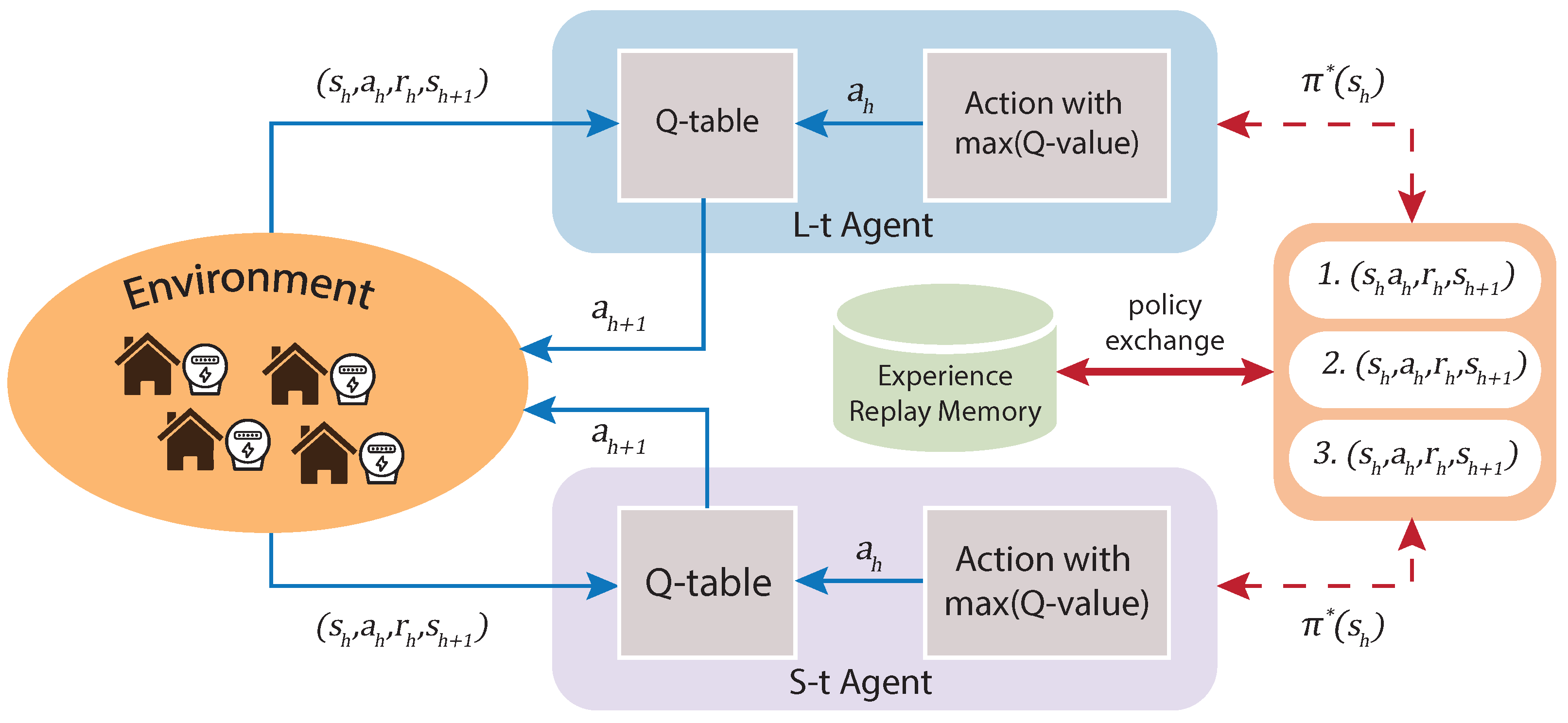
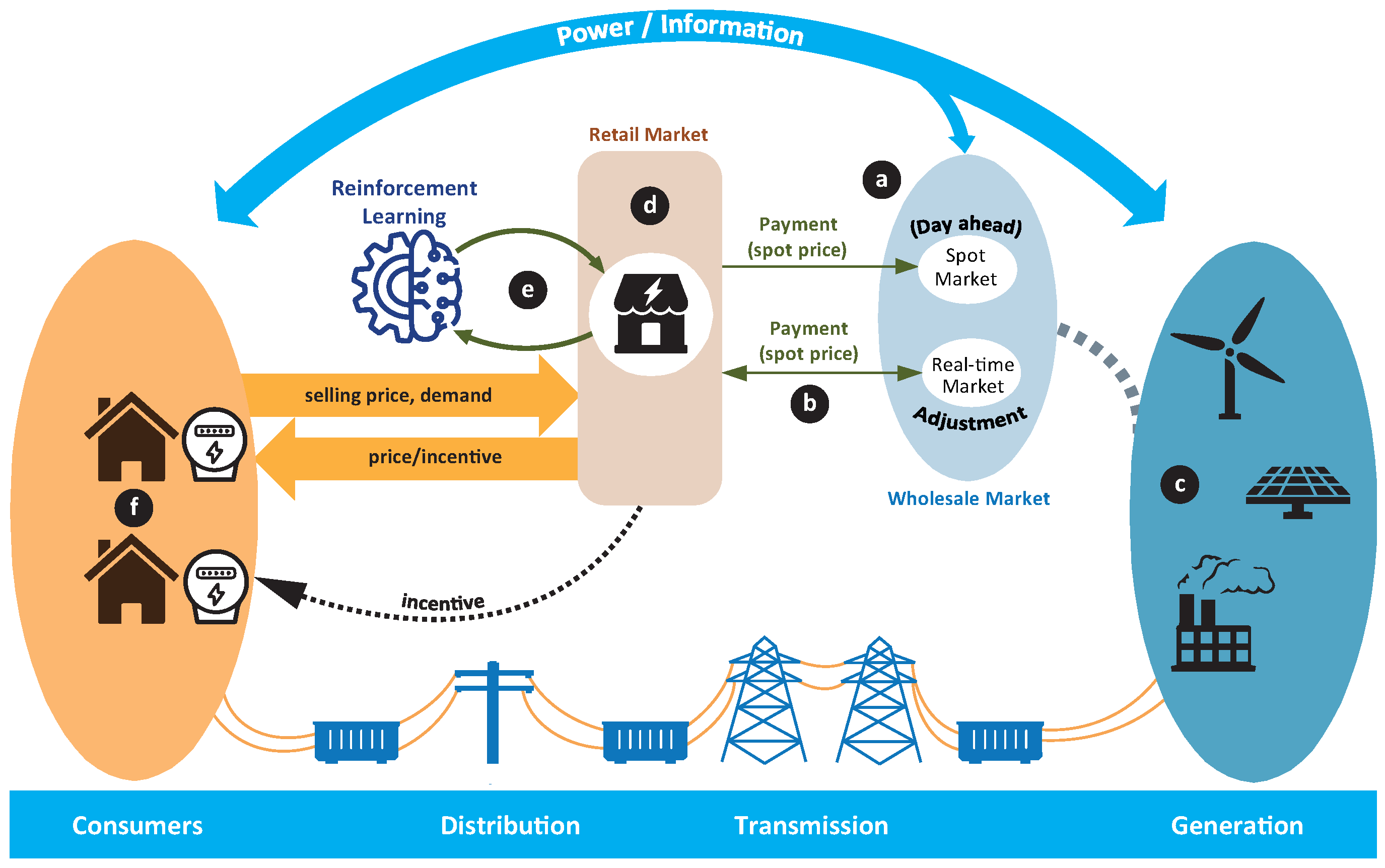
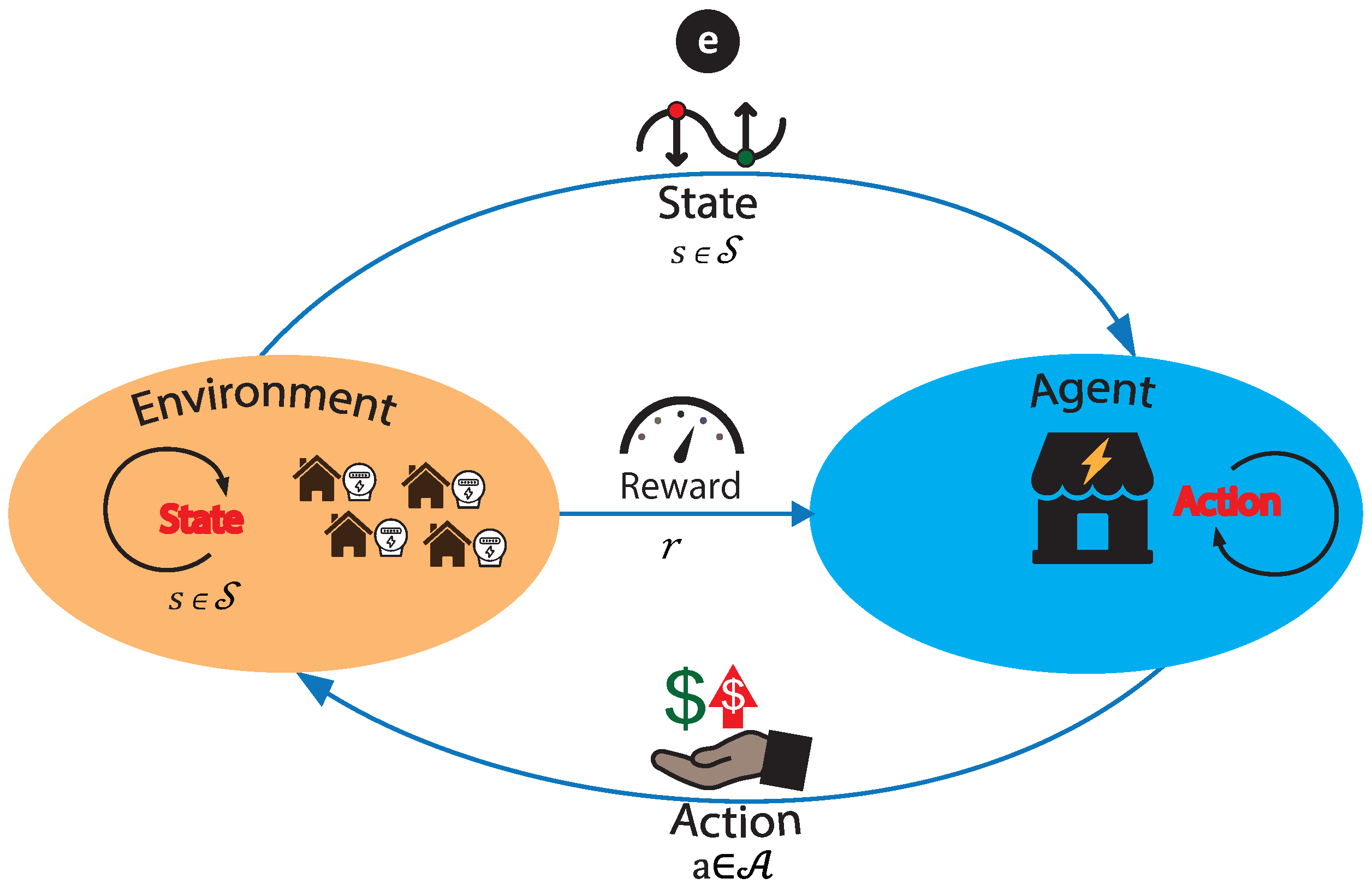
The reinforcement learning (RL) approach is based on object-directed learning from interaction (agent–environment) much more than other learning approaches within machine learning. Specifically, the learning algorithm has no specific actions to perform but must discover which actions will produce a more significant reward through trial and error. That is the goal of the algorithm: to maximize the reward. Furthermore, such actions may affect immediate and future rewards, as current actions will figure out future scenarios. Thus, in each state, the environment makes available a set of actions from which the agent will choose. The agent influences the environment through these actions, and the environment can change state in response to the action of the agent. Next, the process mentioned above is graphically summarized in Figure 1.
Accordingly, it was found that one of the techniques that best understands consumer preferences in a dynamic environment is RL, which is in fact state-of-the-art approach focused on this method. Consequently, articles that consider DR programs based on prices and incentives, consumer satisfaction, RL, consumer classification, and application in practical cases were analyzed in depth.
In [40], an RL architecture is proposed for the best control of HVAC air conditioning systems of an entire building to save energy considering thermal comfort while taking advantage of demand response capabilities. The work mentioned above achieves a maximum weekly energy reduction of up to 22% by applying RL compared to a reference controller. In contrast, the feasibility of applying deep reinforcement learning to control an entire building for demand response purposes is proven. Thus, average power reductions (or increases) of up to 50% were achieved, considering the limits of acceptable comfort. It has been found in these works that the use of applications is improved. For example, in [8], a method is proposed for managing a multipurpose energy storage system (ESS) to participate in response programs for the demand with RL. The work above focuses primarily on industrial consumers to provide them the opportunity to obtain added profits through market participation in addition to offering an improvement for the management of electrical loads. This paper also explores the benefits of using ToU rates, explicitly showing that consumers can obtain more benefits due to changing their consumption from one-time slot to another with a lower price.
Similarly, a neural network is established in [51] to build a series of strategies to obtain control actions in discrete time. For this, RL is used as support to determine a policy that establishes the optimal point for the thermostat configuration. One of the noteworthy features developed by the author is the development of a new objective function truncation method to limit the size of the update step and improve the robustness of the algorithm. In addition, a DR strategy was formulated based on electricity prices according to the time of use, which considers factors such as the environment, thermal comfort, and energy consumption; the proposed RL algorithm is used to learn the thermostat settings in DR time.
In [52], the author proposed a centralized control strategy utilizing a single-agent reinforcement learning (RL) algorithm known as a soft actor critical for optimizing electrical demand across multiple levels, including individual buildings, clusters, and networks. This approach diverges from traditional rule-based control methods, which typically focus on optimizing the performance of individual buildings. Thus, the evaluation of the proposed controller revealed a cost reduction of approximately 4%, with a maximum decrease of 12%. Additionally, daily peaks in electrical demand were found to be lowered by an average of 8%, resulting in a decrease in the peak-to-average ratio of 6–22%. However, it is essential to note that the study also highlights a possible issue with price-based programs, stating that these approaches can sometimes lead to unintended increases in demand during periods of low electricity prices. Despite this, the study also notes that the adoption of multi-agent coordination in demand response applications has not been widely adopted in recent years, possibly due to the lack of understanding of its potential benefits in reducing peak demand or altering daily load profiles.
A DR algorithm based on dynamic prices for smart grids is presented in [53]. Furthermore, the development and formulation of prices to deal with high and highly variable bid prices in the context of RL are shown in this paper. For this, an hourly real-time demand response approach is used. One of the advantages pointed out by the author is that with this algorithm, reliability support is provided to the system, and it achieves a general reduction in energy costs in the market. At the same time, the approach allows flexibility for the system to react quickly to supply demand and correct differences in the energy balance. In addition, a method presented supplies incentives to reduce energy consumption; this occurs when market prices are high, or if the system reliability is at risk.
One of the motivations presented by the author to choose RL is the solution to the problem of making decisions that occur stochastically and thus being able to maximize an immediate and cumulative reward. The scenario presented has a single centralized network operator that keeps, installs, and manages the electrical system. In addition, an electricity service provider is formed of residential, commercial, and industrial consumers. Therefore, the supplier plays a fundamental economic role in the energy supply since it buys the energy from the wholesale market and sells it to consumers at retail prices.
Likewise, [54] presents a multi-agent reinforcement learning (MARL) algorithm for addressing the challenges of community energy management, specifically, peak rebound and uncertain renewable energy generation. The proposed method utilizes a leader-follower Stackelberg game framework, in which a community aggregator serves as the leader, forecasting future renewable energy generation and optimizing energy storage scheduling, updating a Q-table, and initializing a community load profile for all residential consumers. Residential consumers, acting as followers, predict their own renewable energy generation, and schedule home appliances through a sequential decision-making process, utilizing their own individual Q-tables. The proposed MARL algorithm was extensively evaluated against state-of-the-art methods and was shown to be more efficient, reducing peak load, average cost, and standard deviation of cost while effectively addressing the uncertainty of renewable energy generation.
A hybrid DR mechanism is developed in [38], which combines prices and incentives in real-time. This hybrid DR mechanism is modeled under the approach of a Stackelberg game. Within this approach, the agents that participate in the mechanism are the network operator, a retailer that performs the functions of a demand aggregator, and finally, the end consumers. Similarly, in [55], these theoretical RL practical feasibility of approaches is shown by implementing an experimental setup. This work, however, does not consider an incentive scheme that reinforces the participation of consumers.
In the same way, in [56], an online pricing method is proposed considering the response of consumers as unknown, for which the RL approach is used as a tool for decision-making, offering the best incentives. In this work, it is considered that the response behavior of the consumers is unknown, which complicates the resolution of the problem with economic incentives. Seven deep reinforcement learning algorithms (with a transfer learning approach) are empirically compared in [3]. Limitations in the RL and DR studies are highlighted here, including methods for comparing methodologies and categorizing algorithms and their benefits. In [57], the method is framed under the scenario in which the long-term response of consumers is unknown, thus, the author proposes an online pricing method, where long short-term memory (LSTM) networks are combined with a reinforcement learning approach to perform the virtual exploration. In addition, LSTM networks are used to predict the response of the consumer, and through reinforcement learning, the response of the consumer is framed to find the best prices to maximize total benefit and avoid the adverse effects of myopic optimization on RL.
The author in [58], focuses on solving the industrial consumer demand response problem; the need for these schemes is evident due to the size of consumption in the industrial sector compared to the residential or commercial one. In this article, the author proposes a demand response scheme based on multi-agent deep reinforcement learning for the energy management of the components of a discrete industrial process. Here, the simulation results showed that the presented demand response algorithm can minimize electricity costs and support production tasks compared to a non-demand response benchmark.
The articles that include the theme of reinforcement learning are extensively reviewed in [59], emphasizing those algorithms used to solve each problem. In addition, the contribution made by the research mentioned above is that of proposing a basic framework to help standardize the classification of demand response methods. In this extensive investigation, the author briefly deduces that although many articles have considered human comfort and satisfaction as part of the control problem, most have investigated single-agent systems in which electricity prices do not depend on electricity demand energy. These characteristics do not represent the electricity real-world behavior of markets since electricity prices strongly depend on demand. The maximum demand can be shifted instead of reduced by modeling these characteristics.
Among the articles that concentrate their study on electric heating is [60], in which a model that focuses on improving the reduction in carbon emissions and the use of RES is presented. Therefore, this study uses the Weber–Fechner law and a clustering algorithm to build quantitative models of demand response characteristics. In addition, a deep Q network is used to generate dynamic prices for demand aggregators. Specifically, this study considers the quantification of consumer behavior of demand response participants and the differences between consumers. Finally, intelligent electric heating management can provide a favorable environment for demand response.
As has been already mentioned, demand response improves grid security by supplying flexibility to the electricity system through the efficient management of consumer demand while supporting the real-time balance between supply and demand. Thus, with the large-scale deployment of communication and information technologies, distributed digitalization, and the improvement of advanced measurement infrastructures, approaches based on copious amounts of data, such as multi-agent reinforcement learning (MARL), are widely relevant in solving demand response problems.
Due to the massive interaction of data, it is expected that these management systems can lead to significant threats from an information security perspective. For this reason, in [61], the author suggested a robust adversarial multi-agent reinforcement learning framework for demand response (RAMARL-DR) with increased resilience against adversarial attacks. Therefore, the process contemplates formulating a scenario in which the worst case of an adversary attack is simulated. In this case, in addition to the benefits of demand response, it is possible to improve the resilience of the electrical system.
The impact of demand response in a long-term scenario is evaluated in [62], using a model from the Portuguese electricity system in the OSeMOSYS tool. Three scenarios were analyzed to obtain the potential long-term demand response, which differs by the carbon emissions restrictions. This work showed the potentiality of the demand response algorithm to face the problems of optimal management of resources in scenarios with a high penetration of RES derived from the energy transition.
Similarly, in [50], an incentive-based DR program with modified deep learning and reinforcement learning is put forward. First, a modified deep learning model based on a recurrent neural network (MDL-RNN) was proposed, which identifies the future uncertainties of the environment by forecasting the wholesale price of electricity, the production of photovoltaic (PV) sources, and the consumer load. In addition, reinforcement learning (RL) was used to obtain the optimal hourly incentive rates that maximize the profits of the energy service of providers and consumers.
In the literature, there are also hybrid methods that combine the reinforcement learning approach with methods such as those based on rules, a sample of them is [63]; this study investigates the economic benefits of implementing a reinforcement learning (RL) control strategy for the participation in an incentive-based demand response program for a cluster of commercial buildings. The performance of the RL approach is evaluated through comparison with optimized rule-based control (RBC) strategies, and a hybrid control strategy that combines both is also proposed. The study results indicate that while the RL algorithm is more effective in reducing total energy costs, it is less effective in fulfilling demand response requirements. On the other hand, the hybrid control strategy, which combines RBC and RL, demonstrates a reduction in energy consumption and energy costs by 7% and 4%, respectively, compared to a manually optimized RBC and effectively meets the constraints during incentive-based events. The proposed hybrid approach is discussed as a trade-off between random exploration and rule-based expert procedures that can effectively handle peak rebound and promote incentive-based demand response programs in clusters of small commercial buildings.
Within the bibliography, approaches that contemplate the electrical restrictions of networks, as in [64], have also been found where a demand response approach based on batch reinforcement learning is formulated. This approach has the objective of avoiding violations of restrictions to the distribution network. Consequently, through the adjusted Q iteration, the author calculates a secure network policy through historical measurements of load aggregators. Thus, the wide use of the reinforcement learning approach to deal with frequency regulation problems is shown in this study. It is also interesting to mention the vital adaptability for unknown electrical networks achieved by using these artificial intelligence-based approaches.
The demand response methodology not only shows promising results for the electricity market but some studies have also demonstrated its significant relevance to achieving benefits for the actors involved in a supply process, as is the case of the natural gas market. For example, in [65], the point mentioned earlier was demonstrated in this approach, like the electricity market. Furthermore, demand response is used for predictive management in the multilevel natural gas market. In this case, it is shown that it is possible to achieve a better trade-off between supplier profits, gas demand volatility, and consumer satisfaction. In addition, the author developed a model based on the Markov decision process to illustrate the dynamic optimization of energy prices. In that way, the results indicated that the proposed method can achieve the objectives of peak reduction and valley filling in different periods.
Accordingly, a model that helps consumer contribution to DR programs is developed in this paper by combining the price-based DR approach with an incentive proposal. Furthermore, this model is framed within modern AI techniques, specifically reinforcement learning (RL). Consequently, the contribution of this work to the state of the art is its proposal of a novel DR model that combines prices and incentives (PB-IB-DR) to efficiently manage the active response of the end-consumer demand with reinforcement learning.

2.6. Research Gaps and Contributions

This work draws its contribution to the state of the art from an extensive investigation of many previous works. The methodology includes the search through the keywords: “price-based,” “incentive-based,” “short-long term,” “demand response,” and “reinforcement learning,” resulting in highly related articles published after the year 2016, which are shown in Table 3.
From the state of the art, the following unresolved problems stand out:
  • Although there is research that considered real-world data in future scenarios that show promising results, there is still a lack of a complete methodology that considers the characteristics of electricity markets, such as the difficulty in sending signals to consumers (satisfaction), the various rate options, price rates, incentives, and subsidies.
  • The application of RL algorithms in demand response problems is a recent field of research that has not been fully developed from a long-term perspective yet.
  • Research regarding RL in demand response has been applied in ideal scenarios; therefore, neither market aspects nor the contextualization of an application framework is considered.
  • Most investigations do not contemplate different schemes and price rate options, such as the time of use scheme, which allows a better transition and insertion of new changes in the network, such as the massive insertion of RES or electro-mobility.
  • Current methods have been successful in reducing peak rebound events; however, these methods do not fully incorporate the modeling of consumer behavior in terms of satisfaction and comfort. This would enable a more accurate formulation of prices and incentives.
Thus, in this paper is introduced a DR scheme that integrates schemes based on prices and incentives, motivating consumers to change their electricity consumption patterns, which results from considering consumption satisfaction. It is also intended to establish an optimal rate of prices and incentives in the context of modern markets. In addition, tools based on the reinforcement learning framework are used in this work, which increases the penetration rate of RES by providing flexibility to the electrical system and reducing uncertainty in long-term planning. This results from including the signals of the wholesale market in the formulation of rates and incentives and transferring them optimally to consumers. Consequently, the aim is to achieve efficient electrical energy management that allows consumers to manage new system agents, such as electro-mobility and demand aggregators, taking advantage of all available RES. Furthermore, the proposed method adds bidirectional dissatisfaction value for modeling users more accurately and considers their behavior when determining demand response prices offered by the service provider.
Therefore, the purpose of this work is to develop the following:
  • A DR model that combines demand response models based on prices and incentives (P-B and I-B) to efficiently manage the active response of consumer demand considering their satisfaction.
  • A price scheme in real time and by the time of use allows demand management to minimize the variability of electricity supply prices that motivates end consumers to change their consumption patterns.
  • Description and formulation of a market in which the implementation of this study is proposed that includes an adjustment market to support deviation in demand based on short-term benefits for consumers and service providers.

3. Problem Formulation

This work is situated in the context of two markets. Specifically, it has established a wholesale market where generation plants sell their energy in two schemes: on the one hand, a day-ahead market ( d 1 ) Figure 2a closes a settlement over time ( h = 24 ) and, on the other hand, an adjustment market ( d ) Figure 2b is established in real time in a period of h. These two markets enable receiving price signals directly from renewable and all available generation units Figure 2c. Due to these characteristics, this scheme merits partitions in two stages. Thus, on the one hand, a time scale of d a = h H 1 . . . 24 day-ahead ( d 1 ) time steps is denoted by a vector; on the other hand, an hour ( h ) represents each hour at the current day ( d ) represented by r t . It is essential to mention that the vector d a that is obtained is adjusted every hour by the lapse r t , as explained in Figure 3.
Among the actors participating in this market, retailers Figure 2d take on a substantial relevance in this work because the reinforcement learning tool Figure 2e will allow economic planning of the resale of energy from the wholesale market to consumers. For this reason, it is required that the planning must be carried out in the two time periods (day-ahead and real-time, respectively). In this sense, retailers must balance energy supply and demand economically. Traditionally, this balance was achieved by adapting the supply of electrical energy to the demand of the system, that is, the consumers. However, due to the considerations mentioned earlier of the massive penetration of non-conventional RES, it is necessary to have flexibility in demand, which will also allow demand to be adjusted to supply.
Therefore, the retailer needs to obtain information from consumers and market prices (Figure 3). In this sense, on instant h = 0 , the retailer, according to forecast demand sent to the market, receives the price of energy from the spot market for 24 h of the following day. Moreover, in the same way, generators, according to the demand that must be covered, offer prices in the spot market. Once this premise is fulfilled, in the day-ahead stage d a = 1 . . . 24 , the retailer obtains the energy prices of the following day and proceeds to carry out the planning of the energy balance. Therefore, we will focus the analysis on the electricity retailer that economically manages the resale of energy while maximizing its profits. Consequently, for this function, it is necessary to obtain wholesale energy prices from the market for 24 h of the following day. From the consumers Figure 2f, historical and processed data of their demand behavior is required, from that information it is obtained their elasticity, behavior in system peaks, and load factor, among others.
The retailer sends the information from the spot market and consumers to the algorithm. These data constitute the input for the reinforcement learning algorithm, which will process these data, return a price to consumers as an output, and predict the variation in demand (demand response). Therefore, the RL algorithm enables the period t i m e = h ( r t ) since it first calculates an electricity sale price for the 24 h of the following day, which is sent to consumers at t i m e = 24 ( d a ) ; these prices can be received both in a domestic energy management system and directly by consumers. In other words, the consumer may or may not participate in their consumption in the demand response program.
Once consumers receive the 24 prices for the next day, as mentioned, they can plan their consumption according to their elasticity. However, this proposed approach to reinforcing consumer participation also operates in the real-time adjustment market. Therefore, we are now going to focus the analysis on this scenario. At this moment, the algorithm already has historical information on consumers. Therefore, the algorithm can estimate the possible behavior of the consumer, which allows obtaining a priori incentives; these incentives will be sent in connection with a satisfaction function. In this sense, the consumer also receives a finite number of incentives for hours required to change the behavior, and the elasticity has low values; this approach is based on the critical peak price (CPP) mechanism.
For the instant of time t = h ( r t ) , the algorithm compares the estimated behavior of the consumer through the historical ones and, throughout each hour, modifies its elasticity and a proposed factor, called the experience factor, which allows, on the one hand, modifying and personalizing prices to obtain incentives based on the experience of their behavior throughout the day. However, it is essential to point out that the algorithm considers a possible scenario when the consumer does not respond to the demand response program; that is, the consumption is not modified compared to the historical one. In this case, shipping pricing will approximate a less variable and approximate pricing scheme (similar to a ToU time of use scheme). Furthermore, if the consumer does not respond to this simplified pricing scheme, the scheme will eventually convert to a fixed pricing scheme, known as a flat rate. Here, the question could arise as to whether the scheme could first consider a flat rate and then become a real-time hourly price scheme, an action that the algorithm can effectively carry out. However, it is not the focus of this work since the proposed hypothesis considers, in the first instance, that the consumer is willing to participate in modifying the electricity demand.

3.1. Reinforcement Learning Overview

The reinforcement learning (RL) approach addresses the problem of how an agent can maximize the benefit that it can obtain in an environment by perceiving the reaction (reward) that a state (state) gets due to an action (action). The objective of this agent is to learn which set of actions (policy) will allow the highest performance (return) from the environment, so it is understood that each action modifies the environment; this process is based on interactive learning between the agent and the environment. The aforementioned is presented in Figure 4.
During reinforcement learning, the agent constantly interacts with the environment. First, the agent acquires the state and uses this state to generate an action and a decision. Then this decision will be made in the environment, which will generate the next state and the reward for the current action according to the decision made by the agent. The purpose of the agent is to obtain as much reward as possible from the environment.
Reinforcement learning is the third primary machine learning method besides supervised and unsupervised learning. For example, supervised learning is based on learning from a training set provided by an external supervisor. Meanwhile, unsupervised learning is a typical process of finding hidden structures in unlabeled data. Finally, reinforcement learning focuses more on learning than on results purely from the interaction between the agent and the environment, which poses a unique challenge defined as the balance between “exploitation” and “exploration”, which is to achieve a balance between the actions you know and new actions unknown.
Consequently, reinforcement learning is based on a trial-and-error learning interaction, where learning generally does not have direct orientation information; the agent must continuously interact with the environment to obtain the best policy (Policy) through trial and error. Moreover, in this approach, rewards are delayed; that is, instructional information for reinforcement learning is rarely provided up front and is often provided after the fact (last state).
Within the elements that make up the reinforcement learning approach is the environment, an external system in which the agent is located; here, the agent can perceive a particular system and perform specific actions depending on the state it perceives. Furthermore, the agent is a system embedded in the environment that can change its state through its actions. Therefore, at first it is necessary to build a model that considers these elements. It is necessary to model the consumers with their respective benefits for the environment.

3.2. Modeling of Electricity Consumers

The consumer model comprises a chain of elements that make up the individual benefit. Within this chain of elements is found, for example, the value of the energy purchased from the service provider (energy price), the incentive granted by the demand response (reduction or increase), the decrease or increase in demand in each period, and the cost of dissatisfaction. In this work, two types of consumers have been considered: on the one hand, consumers who buy energy through an RTP and on the other hand, consumers who purchase energy through a time of use price scheme ToU. In this context, RTP and ToU consumers can be incentivized to perform demand responses. Specifically, the benefit for RTP consumer is presented in Equation (1), and the formulation for consumers (ToU) is determined in Equation (7).
U b e n u , h = u = 1 U h = 1 H η u · ( Δ C u , h · μ u , h ) ( C u , h · r u , h ) + η u ( 1 ρ ) · ( ϕ u , h )
ϕ u , h ( C u , h ) = β u , h 2 · ( C u , h ) 2 + C u , h
β u , h > 0
η u = ( ν u , e n d ν u , s t ) · ν u , D R ν t o t
where β represents the preference of consumer regarding the willingness to perform demand response; therefore, the higher value indicates that the consumer adopts a conservative stance to reduce consumption the above is shown in Figure 5. In this example, while the value of β increases, the consumer is willing to reduce his consumption for his electricity demand. Consequently, the β factor is a value that must be represented for each consumer. A parameter has also been added to measure experience throughout the execution of the DR model (Figure 3). In this sense, ν u , s t represents the time defined in hours in which the first economic incentive is sent to each consumer, while ν u , e n d defines the current or final time of the last incentive sent to consumers from the provider. In addition, the term ν t o t represents the experience of the consumer participation in the DR model while the time incentives are applied. Finally, ν u , D R represents the number of times the consumer participated in the DR model as a member. Consequently, η u is a parameter that will reinforce those incentives sent by the service provider to consumers who actively participate in reducing their demands.
However, within this approach, it is necessary to analyze not only the decrease in consumption but also the increase and its influence on consumer satisfaction; that is, a model that considers these two scenarios is necessary, for example, the above is shown in Figure 6. On the one hand, the model considers the scenario where a reduction in demand consumption represents a cost of dissatisfaction that increases when this decreases. On the other hand, it is considered when the consumers receive an economic incentive to increase their consumption, which reduces the cost of dissatisfaction.
ϕ u , h ( P u , h , C u , h ) = P u , h · β u , h ( C u , h P u , h ) 3 C u , h
β u , h > 0
ϕ u , h represents the consumer satisfaction function; this function quantitatively models satisfaction based on the difference between the nominal demand and actual consumption of consumers. If the consumption is less than the demand, the value of the function is positive, which means that the consumers are not satisfied, which results in a decrease in the representative cost for the final consumer. In addition, the function value increases faster as the actual load decreases, representing rational consumer behavior concerning demand response. On the other hand, if the consumption is greater than the demand of consumers, the value of the function is negative, which means that the consumers are satisfied. However, the slope of function decreases as the actual load increases because consumers will not be infinitely more satisfied when using more electricity. This bidirectional satisfaction function denotes a key attribute that confers a significant benefit in mitigating peak rebounding effects, mentioned in the Demand Response (DR) approaches outlined in [43,52,54,63]. Finally, when the actual load is equal to the consumer demand, the value of the function is zero. Then, for those consumers who are willing to add themselves to an hourly rate that varies depending on use, the following Equation (7) is established [66,67]:
U T o U b e n u , h = u = 1 U h = 1 H η u · ( Δ C T o U u , h · μ u , h ) ( C T o U u , h · r u , h ) + η u ( 1 ρ ) · ( ϕ u , h ) ,
where r u , h represents the retail price offered to consumers by energy providers. This price can vary hourly or by time slots. It is proposed to carry out a previous grouping that will serve as input for both the short-term and long-term reinforcement learning algorithm. Consequently, consumers have been classified based on their behavior and influence on the demand curve. The classifier uses weight variables such as the concurrency and coincidence factors. These indexes represent the inverse diversity factor and the relationship between the demand of each consumer and the maximum demand set of consumers over the sum of the maximum individual demands expressed as a percentage. The influence of the coincidence factor is determined by the habits of the population and the climatic conditions, among others.

3.3. Modeling of Service Provider

In this sense, the electricity reseller will be called a service provider (SP). In this work, the SP, aggregator, or marketer has been modeled as an agent of the electricity market that obtains energy from the wholesale market in the two proposed schemes. On the one hand, the SP buys power one day before in the “day-ahead” market, and on the other hand, it also buys energy every hour in the “real-time” market. In this sense, the electricity purchased in either of the two markets is then sold to distribution consumers. Therefore, the SP will obtain its benefit from this resale of energy. However, as explained above, the SP is not in charge of the maintenance and operation of the distribution networks; it only fulfills the function of energy commercialization. Consequently, the utility of the business of SP results from the sale of energy in both short- and long-term markets. Therefore, the function that represents its utility is expressed as follows:
S P d a b e n u , h = u = 1 U h = 1 H ( Δ C u , h · r u , h ) + ( Δ C T o U u , h · r T o U u , h ) Ω · μ u , h · ( Δ C u , h + Δ C T o U u , h ) ( C u , h · z h d a )
Ω = 0 S P b e n t o t S P b e n r e f 1 S P b e n t o t > S P b e n r e f
S P b e n t o t = u = 1 U h = 1 H S P d a b e n u , h
S P r t b e n u , h = u = 1 U h = 1 H ( Δ C u , h · r u , h ) + ( Δ C T o U u , h · r T o U u , h ) μ u , h · ( Δ C u , h + Δ C T o U u , h ) ( C u , h · z h r t )
μ m i n μ u , h μ m a x
In this sense, it is necessary to note that the methodology considers wholesale market prices in the day-ahead and real-time markets. Therefore, a neural network has been used to predict this price and thus reduce the uncertainty of wholesale price. With this, it will be possible to estimate the utility the SP will obtain under the two schemes. In addition, data from the Argentine electricity market has been used [68]. The estimation of these parameters using a neural network under the following parameters. For prediction error measurement, the root-means-square error is used as follows.
R M S E = i = 1 n ( y i y i ^ ) 2 n
where y i is the expected result and y i ^ is the model prediction.

3.4. Objective Function

The objective function presented below considers the maximization of each of the individual benefits, that is, for consumers under a real-time price scheme and those who purchase energy from the supplier through a price defined by time slots.
r t d a = m a x u = 1 U h = 1 H ( U b e n u , h + U T o U b e n u , h + S P d a b e n u , h )
r t r t = m a x u = 1 U h = 1 H ( U b e n u , h + U T o U b e n u , h + S P r t b e n u , h )

3.5. Demand Response Scheme

A detailed methodology scheme used in this work is presented in this section and is described in Figure 7. Once the data from the meters installed in each consumer are obtained, the elasticity is calculated as determined in [69]. Once the elasticity calculation is performed, these data are classified using the k-means grouping algorithm. For this purpose, the pseudo-code used for the grouping is presented in the Algorithm 1.
Algorithm 1: Cluster of consumers C-ABD.
Energies 16 01466 i001
In this sense, the characteristics that have been useful for clustering the typical curves of consumer demand have been the coincidence factors, the same ones shown in Figure 8.
In this context, with the data resulting from the classification and the data set of the wholesale market, the input data are made up, which, in this case, will be those that make up the inputs of the two reinforcement learning approaches, on the one hand, of short term and long term. Therefore, in this sense, reinforcement learning is proposed at each stage. However, on the other hand, the RL approach focuses on the interaction between the agent and environment rather than learning techniques such as supervised and unsupervised.
For this reason, it is necessary to formulate, in the first instance, the environment; in this case, it is made up of the energy measurements of each consumer. On the other hand, there is the agent, which comprises processing from the perspective of the service provider, aggregator, and marketer. Therefore, these two agents interact in a discrete-time sequence t T . When the agent observes the change in the RL environment due to an action, it establishes state observations. A state S comprises all the parameters the marketer or demand aggregator obtains from the consumer. The agent actions A are the prices/incentives offered to the consumers. Finally, the final reward of the approach was proposed as the set of rewards (benefits) presented in Equations (19) and (20), denoted as r t .
S d a : [ Δ C u , h , Δ C T o U u , h , Z h d a , C u , h , ϕ u , h ]
S r t : [ Δ C u , h , Δ C T o U u , h , Z h r t , C u , h , ϕ u , h ]
A u , h : [ μ u , h , r u , h , r T o U u , h ]
u U h H r t d a = u U h H r U b e n u , h + u U h H r U t o u b e n u , h + u U h H r S P d a b e n u , h
u U h H r t r t = u U h H r U b e n u , h + u U h H r U t o u b e n u , h + u U h H r S P b r t e n u , h
Within these actions, it is essential to define a policy π . This policy is a rule that the agent must use to decide what to do given the knowledge of the current state of the environment since it represents the function that maps the action A to the state S .
Q s d a u , h , a u , h = Q s d a u , h , a u , h + α · [ r s d a u , h , a u , h + γ · Q s d a u , h + 1 , a u , h + 1 Q s d a u , h , a u , h ]
Q s r t u , h , a u , h = Q s r t u , h , a u , h + α · [ r s r t u , h , a u , h + γ · Q s r t u , h + 1 , a u , h + 1 Q s r t u , h , a u , h ]
Therefore, the pseudo-code shown in Algorithm 2 is characterized by having a memory that stores the optimal policies of the L-t RL algorithm. This tuple of policies serves as a support so that in the first instance, the agent S-t can start without considering an e-greedy policy but proceed with this a priori tuple and then start iterating, maximizing the reward. Every time the agent obtains an optimal policy, the S-t Q-learning algorithm stores its tuple to make a trade-off between the two short-term and long-term approaches. Therefore, as in Figure 9, Agent L-t obtains from the environment, state, and rewards s h , a h , r h , s h + 1 due to the actions a h + 1 . With this information, the Q-table is obtained. In addition, through the policy interaction approach, the actions that maximize the Q-values are found, that is, the rewards r h of Q * s h , a h As an output of the L-t Q-learning algorithm, the optimal policy π * S h is obtained and stored in the replication memory of the experience. Once the temporality change has been made, as explained in Figure 2, the agent searches for the actions that maximize the max ( Q - v a l u e ) reward. In this sense, the agent already has part of the previous knowledge and uses the iterations of the L-t agent as input for the optimal policy π * S h search.
Algorithm 2: ERM Q-learning.
Energies 16 01466 i002

4. Result Analysis

4.1. Application Scenario

This work has taken as input data, the data provided by the smart meters of the consumers in a distribution network grid. This electric network is part of an innovation project, “Caucete Smart Grid” This project aims to transform part of the current electrical distribution network of the City of Caucete (placed in the province of San Juan—Argentina) into an innovative and modern network [70]. This update will improve the operation, control, and electrical performance of network. The goals of the project are to contribute to energy efficiency (electricity) and a better quality of service to maximize global and comprehensive benefits for consumers, the electricity company, and society in general, increasing social benefits. In addition, it looks to promote, in turn, the use of RES for electricity generation, such as photovoltaic solar energy. Finally, the ability to provide the system with an advanced measurement infrastructure to show consumption patterns and achieve a sustainable system with innovative strategies is viewed.
This approach will support the “Caucete” smart grid project by enabling or enhancing consumer participation in a demand response program, supplying economic targets for electricity consumers and retailers. For this, the method has been framed within a day-ahead market. On the one hand, a reduction in the consumption price or specific discounts will be achieved for consumers by including incentives (concerning their degree of participation). In addition, it will be possible to provide the electricity system to consumers with active involvement and elastic demand. On the other hand, among the benefits that electricity retailers will obtain is improved planning of its usefulness and having a tool that allows prompt response to events such as a reduction in supply.
Moreover, under this approach, other actors indirectly receive aim from the demand response, as is the case of operators and electricity companies that will be able to count on a flexible tool that allows them to face the challenges of technological changes such as decarbonization or the entry of agents such as electric vehicles, and so on. Thus, electric companies can plan their expansion better by having a DR program. Specifically, by having an elastic demand, it will be possible to balance the loads to avoid the underuse of equipment in electrical infrastructure. Finally, the electricity system will be able to use its energy resources better to maximize the use of RES [71]. As mentioned in this work, the electrical power and electrical consumption measurements come from the “Caucete” smart grid project; therefore, the measurements of each consumer are obtained, and through Algorithm 1, they are classified by their incidence in the peak (internal or external coincidence factor).
First, a consumer whose electricity consumption does not coincide with the peak of the system and occurs after 8:00 p.m. was selected. However, this consumer has its peak between 1:00 p.m. and 7:00 p.m. Therefore, the cluster must detect this behavior and group the consumption curves according to the DR requirements. In this case, in Figure 10 (blue), within the cluster options, a curve that covers the peak of the consumer is no longer considered, which was considered in Figure 10 (red). Finally, the behavior of the different variables is shown in Figure 11.
Likewise, the residential consumer contemplated for this work was selected. The result of the classification for a residential consumer is shown in Figure 12. Furthermore, Figure 13 shows how the classification adequately separates each data set into the corresponding neighborhoods. In addition, since each consumer needs an adequate separation of clusters and a calculation of the number of clusters, the Calinski-Harabasz criterion is used to obtain the optimal number of clusters for each consumer. In this case, for the same consumer, the result is 4, as shown in Figure 14.
The price at which a retailer or aggregator buys energy is needed as input to the algorithm from the wholesale market side (day-ahead market, real-time market). In addition, as shown in Figure 7, it is required to forecast these values to reduce the volatility of these prices through the data estimation and forecasting process. Therefore, the prices offered by the national energy regulator (CAMMESA) have been taken as a reference. The data was estimated through an intelligent network to forecast time series.
To predict the values of future time steps of step, we trained a stepwise regression LSTM network, where the responses are the training steps with values changed by a single action. The data was configured as 90% for training and the other 10% for testing. In addition, the LSTM layer with 128 hidden units was used. This LSTM network was tested with the following parameters, with three algorithms, namely Adam, SGDM, and RMSProp. This test shows that the algorithm with the best result in terms of error (RMSE) is Adam; therefore, this algorithm was chosen, Figure 15.

4.2. Long-Term Q-Learning

After obtaining the price forecast data with the consumer classification using the C-ABD algorithm, the L-t Q-learning algorithm is executed. The typical curves of each consumer are required, and one of the curves resulting from the clustering process was selected. Specifically, it is shown in Figure 16 how real-time pricing looks to move away from a flat price signal towards a dynamic pricing scheme. This price variation reduces consumer peaks, considering maximizing at the same time the benefits of the consumer and the marketer or aggregator.
As shown in Figure 16, in addition to the RTP and ToU prices, a static ToU rate was proposed that considers the schedules previously established by the national electricity regulator. In this case, it is necessary to mention that the ToU dynamic pricing scheme can be established at any time, considering three price levels to facilitate consumer participation.
Figure 17 shows how, by including a wholesale market price signal and matching factors, the share of consumer demand is achieved to reduce the peak of the system (set of consumers). Furthermore, it is observed that the approach no longer recognizes the peak of consumers as the target to reduce. Therefore, the hours in which consumer demand peaks present moderate price signals against the scenario without considering coincidence factors. These scenarios are presented in Figure 18, as well as the variation in demand due to the new price signals. It is essential to point out that the static time of use price signal, in this case, is inefficient because it does not obey the dynamic behavior of demand; this is a feature known in advance. In addition, because the method considers the bidirectional satisfaction expressed in Figure 6, it can be seen how the algorithm offers prices that motivate the consumer to increase their consumption. This characteristic is observed for the first consumption hours of the day. Therefore, it is observed in Figure 17 how the consumer obtains prices that consider an elasticity shown in Table 4 [66].
In this sense, it is shown in Figure 18 that the consumer effectively reduces consumption at the time established as the peak of the system. Therefore, the demand response objective is achieved. On the other hand, because the model offers consumers a lower price than a flat rate, it is observed that in these hours, the electricity consumption tends to increase to a lesser extent, but it fulfills the transfer function of the system peak.
The prices obtained from the reinforcement learning approach result from maximizing the benefits of each of the actors; for this reason, Figure 19 shows the behavior of the accumulated reward for the formulation of demand response prices, considering the first three clusters shown in Figure 12. As can be seen, the algorithm manages to maximize its objective in around 600 episodes. In this case, the algorithm has been configured so that the number of episodes is 1000. In addition, it is observed that the algorithm looks for similar strategies for the three cases, which points to similar growth.

4.3. Long Short-Term Q-Learning

The results of the model, defined in Figure 20, will be presented in this section. For this analysis, the same consumer analyzed in the previous section was taken in the first instance; it will be considered that the consumer has already received a price scheme and responded to the day-ahead signals. Therefore, the model will seek to offer new adjustment prices to promote an even more robust response and sends economic incentives based on new consumer demand to reinforce responses to energy spikes. As can be seen, the consumers have reduced their consumption of it when the system peak is encountered. In other words, the model formulates the incentives by observing the peak of consumers and downplaying the peak of system.
The preceding is because the consumer no longer has excessive consumption during system hours, which allows him to receive price signals according to his behavior. Consequently, the model seeks to reduce the peak of consumers at 10:00 a.m. and encourages them to increase their consumption during off-peak hours. Finally, it can be seen how, with these two approaches, it is possible to encourage consumers to respond to two specific events effectively. On the one hand, the need to reduce the demand peak that coincides with the peak of the system, and on the other, when it is necessary to maximize the load factor of the distribution network by increasing consumer consumption during off-peak hours.
A horizon of four days was established to determine the prediction of the model and the reference consumer data to verify that the algorithm understands the long term. In addition, it verifies that the model transfers data through shared memory between the short and long-term approaches to improve performance and the search for the best solution possible. In this sense, it can be seen in Figure 21 how in the long term, the algorithm finds the best prices to reduce not only the peaks of the system but through incentives; it manages to determine the long-term peak, generating a signal that can even support a direct load control scheme.
In this document, we measured the performance of the proposed pricing schemes based on two metrics. In the first place, the total change in electrical energy per day, called the variation in demand, was taken as a reference. Consequently, this demand variation factor DV considers the relationship between consumption before any demand response action and the same consumption after implementing a demand response scheme. The above factor is expressed in Equation (23).
DV = o r i g C u n e w C u o r i g C u
In addition, we also measured the average load factor of consumers to compare the formulation of prices and if it manages, despite the actions to respond to demand, to improve the load factor. This metric can be extrapolated to a measure that represents the high peak consumer demand and the effectiveness of the pricing scheme in displacing electricity demand. For this, Equation (24) was taken as a reference.
LF = A v L M a x ( L h )
With the indices shown in the previous equations, it has been possible to measure the performance of the presented model; therefore, in this case, the evaluation is presented considering a sensitivity in the elasticity for the same consumer (Figure 22).
Consequently, it is shown as, from a minimum participation value, the real-time and time of use rate presented by the model increases the load factor compared to the demand response that only takes the reduction into account (reference model). In addition, the variation in demand was considered, and it has been possible to determine that, as observed in the graphs in the same way as the previous metric, the rate of time of use offers a better load displacement than the reference model. The hardware and software characteristics of the computer used for the simulation are shown below in Table 5.

5. Conclusions and Future Works

This work proposes a DR model based on prices and incentives (P-B and I-B). The results on consumers demonstrate the importance of considering the coincidence factor of electricity demand and thus be able to characterize each behavior of consumers, to focus on the appropriate demand response strategy. This originates from the fact that by considering the peaks of the system, a better signal to the consumer can be obtained to perform “peak clipping.” The short- and long-term approach presented for a combined real-time and day-ahead market demonstrates the usefulness of considering incentives that reinforce consumer behavior and demand adjustment. Furthermore, the long-term functionality presented by the model offers the advantage of adjusting the demand response objectives.
Finally, this work proposes a Q-learning model with memory exchange from the short term to the long term; this approach allows to focus on the economic incentives of the consumers and improves the formulation of prices in a real-time market as well as for the schemes of prices designed to cover the long term such as the time of use price scheme. Consequently, the improvement of the load factor of consumers was demonstrated, reflecting the effectiveness of the model in displacing the consumption peaks.
In future works, we have seen the need to consider various types of consumers and focus the study on the particularities of elasticity. In addition, it is necessary for demand response programs to be effectively implemented in distribution systems to take into account tariff aspects and the influence of nodal prices. Therefore, a tariff model that complements this presented work is already under development. Instead, it is essential within the characterization of consumers and demands it is necessary to consider various types of satisfaction factors for each of the consumers, in addition to the analysis of their influence on the model presented.
This study presents a new methodology, including the introduction of a bidirectional satisfaction factor and a real-time adjustment market, that is aimed at balancing the energy supply and demand. However, it is acknowledged that additional research is required to further refine and improve the proposed methodology to more effectively address the potential for peak rebound effects in this context.

Author Contributions

Conceptualization, E.J.S. and M.E.S.; methodology, E.J.S. and M.E.S.; formal analysis, E.J.S. and M.E.S.; investigation, E.J.S. and M.E.S.; writing—original draft preparation, E.J.S. and M.E.S.; writing—review and editing, E.J.S., M.E.S. and M.J.; supervision, M.E.S.; project administration, M.E.S. All authors have read and agreed to the published version of the manuscript.

Funding

This research received no external funding.

Institutional Review Board Statement

Not applicable.

Informed Consent Statement

Not applicable.

Data Availability Statement

Not applicable.

Acknowledgments

This work was supported by the German Academic Exchange Service with a scholarship for a Ph.D. scholarship of Funding programme/-ID: Third Country Programme Latin America, 2018 (57399476).

Conflicts of Interest

The authors declare no conflict of interest.

Abbreviations

The following abbreviations are used in this manuscript:
hThe number of hours per day H = 24
d a The time scale of d a = h 24
r t Real-time framework h = 1
sState of the environment at time t , s S d a and s S r t
rRL-Reward includes benefits for consumers and service providers
a Actions from agent to environment a A
U b e n u , h Consumer benefit with real-time pricing scheme u = 1 , , U
USet of Consumers U = 12
η u The participation factor of each consumer in each hour:
limited by ν u , i n i < ν u , e n d < ν u , t o t
ρ Weighting factor ρ 0 , 1
Δ C u , h Decrease or increase demand per consumer with real-time price at a specific time
μ u , h The incentive for each consumer at a specific time
r u , h Real-time price for each consumer
ϕ u , h Dissatisfaction cost of each consumer
β u , h The dissatisfaction cost reflects acceptance of consumers of the DR
Δ C T o U u , h Decrease or Increase in Demand per ToU consumer in a specific time slot
C T o U u , h Demand per consumer ToU in a specific time slot
U T o U b e n u , h Consumer benefit with price scheme ToU u = 1 , , U
S P d a b e n u , h Service Provider Benefit (day-ahead)
Ω Incentive binary variable
z h d a Wholesale price from Day-ahead market
S P b e n t o t Sum of Service Provider Benefits (day-ahead, real-time)
S P r t b e n u , h Service Provider Benefit (real-time)
r t d a , r t r t The day-ahead and Real-Time Reward
C u Electric Energy Consumption per consumer
P h u Peak power per consumer
M p u Peak demand of each consumer
C k The cluster of each category
QQ-table of Q-Learning
ECoefficient of elasticity per consumer
D V Demand variation factor
L F Load Factor

References

  1. Neves, D.; Pina, A.; Silva, C.A. Assessment of the potential use of demand response in DHW systems on isolated microgrids. Renew. Energy 2018, 115, 989–998. [Google Scholar] [CrossRef]
  2. Cardoso, C.A.; Torriti, J.; Lorincz, M. Making demand side response happen: A review of barriers in commercial and public organisations. Energy Res. Soc. Sci. 2020, 64, 101443. [Google Scholar] [CrossRef]
  3. Peirelinck, T.; Kazmi, H.; Mbuwir, B.V.; Hermans, C.; Spiessens, F.; Suykens, J.; Deconinck, G. Transfer learning in demand response: A review of algorithms for data-efficient modelling and control. Energy AI 2021, 100126. [Google Scholar] [CrossRef]
  4. Nakabi, T.A.; Toivanen, P. Deep reinforcement learning for energy management in a microgrid with flexible demand. Sustain. Energy Grids Netw. 2021, 25, 100413. [Google Scholar] [CrossRef]
  5. Parrish, B.; Gross, R.; Heptonstall, P. Energy Research & Social Science On demand: Can demand response live up to expectations in managing electricity systems? Energy Res. Soc. Sci. 2019, 51, 107–118. [Google Scholar] [CrossRef]
  6. Parrish, B.; Heptonstall, P.; Gross, R.; Sovacool, B.K. A systematic review of motivations, enablers and barriers for consumer engagement with residential demand response. Energy Policy 2020, 138, 111221. [Google Scholar] [CrossRef]
  7. Blanke, J.; Beder, C.; Klepal, M. An Integrated Behavioural Model towards Evaluating and Influencing Energy Behaviour—The Role of Motivation in Behaviour Demand Response. Buildings 2017, 7, 119. [Google Scholar] [CrossRef]
  8. Oh, S.; Kong, J.; Yang, Y.; Jung, J.; Lee, C.H. A Multi-Use Framework of Energy Storage Systems Using Reinforcement Learning for Both Price-Based and Incentive-Based Demand Response Programs. SSRN Electron. J. 2022, 144, 108519. [Google Scholar] [CrossRef]
  9. Deng, R.; Xiao, G.; Lu, R.; Chen, J. Fast distributed demand response with spatially and temporally coupled constraints in smart grid. IEEE Trans. Ind. Inform. 2015, 11, 1597–1606. [Google Scholar] [CrossRef]
  10. Arias, L.A.; Rivas, E.; Santamaria, F. Preparation of Demand Response Management: Case Study; IEEE: Santiago de Cali, Colombia, 2018; pp. 1–6. [Google Scholar] [CrossRef]
  11. Kim, G.; Park, J. 2018 IEEE International Conference on Big Data and Smart Computing A Study on Utilization of Blockchain for Electricity Trading in Microgrid. In Proceedings of the 2018 IEEE International Conference on Big Data and Smart Computing (BigComp), Shanghai, China, 15–17 January 2018; pp. 743–746. [Google Scholar] [CrossRef]
  12. Bui, V.H.; Hussain, A.; Kim, H.M.; Member, S.; Hussain, A.; Member, S. A multiagent-based hierarchical energy management strategy for multi-microgrids considering adjustable power and demand response. IEEE Trans. Smart Grid 2018, 9, 1323–1333. [Google Scholar] [CrossRef]
  13. Cui, H.; Zhou, K. Industrial power load scheduling considering demand response. J. Clean. Prod. 2018, 204, 447–460. [Google Scholar] [CrossRef]
  14. Sonsaard, P.; Ketjoy, N.; Mensin, Y. Market strategy options to implement Thailand demand response program policy. Energy Policy 2023, 173, 113388. [Google Scholar] [CrossRef]
  15. Panwar, L.K.; Konda, S.R.; Verma, A.; Panigrahi, B.K.; Kumar, R. Demand response aggregator coordinated two-stage responsive load scheduling in distribution system considering customer behaviour. IET Gener. Transm. Distrib. 2017, 11, 1023–1032. [Google Scholar] [CrossRef]
  16. Cortina, J.J.; López-Lezama, J.M.; Muñoz-Galeano, N. Modelo de Interdicción de Sistemas de Potencia considerando el Efecto de la Respuesta a la Demanda. Inf. Tecnológica 2017, 28, 197–208. [Google Scholar] [CrossRef]
  17. Hao, H.; Corbin, C.D.; Kalsi, K.; Pratt, R.G. Transactive Control of Commercial Buildings for Demand Response. IEEE Trans. Power Syst. 2017, 32, 774–783. [Google Scholar] [CrossRef]
  18. Tsolakis, A.C.; Moschos, I.; Votis, K.; Ioannidis, D.; Dimitrios, T.; Pandey, P.; Katsikas, S.; Kotsakis, E.; Garcia-Castro, R. A Secured and Trusted Demand Response System Based on Blockchain Technologies; IEEE: Piscataway, NJ, USA, 2018; pp. 1–6. [Google Scholar] [CrossRef]
  19. Yan, X.; Ozturk, Y.; Hu, Z.; Song, Y. A review on price-driven residential demand response. Renew. Sustain. Energy Rev. 2018, 96, 411–419. [Google Scholar] [CrossRef]
  20. Stanelyte, D.; Radziukyniene, N.; Radziukynas, V. Overview of Demand-Response Services: A Review. Energies 2022, 15, 1659. [Google Scholar] [CrossRef]
  21. Ghazvini, M.A.F.; Soares, J.; Abrishambaf, O.; Castro, R.; Vale, Z. Demand response implementation in smart households. Energy Build. 2017, 143, 129–148. [Google Scholar] [CrossRef]
  22. Erdinç, O.; Taşcikaraogvlu, A.; Paterakis, N.G.; Eren, Y.; Catalão, J.P. End-User Comfort Oriented Day-Ahead Planning for Responsive Residential HVAC Demand Aggregation Considering Weather Forecasts. IEEE Trans. Smart Grid 2017, 8, 362–372. [Google Scholar] [CrossRef]
  23. Wang, F.; Zhou, L.; Ren, H.; Liu, X.; Talari, S.; Shafie-Khah, M.; Catalao, J.P.S. Multi-Objective Optimization Model of Source-Load-Storage Synergetic Dispatch for a Building Energy Management System Based on TOU Price Demand Response. IEEE Trans. Ind. Appl. 2018, 54, 1017–1028. [Google Scholar] [CrossRef]
  24. Liu, Y. Demand response and energy efficiency in the capacity resource procurement: Case studies of forward capacity markets in ISO New England, PJM and Great Britain. Energy Policy 2017, 100, 271–282. [Google Scholar] [CrossRef]
  25. Hausman, E.D.; Tabors, R.D. The Role of Demand Underscheduling in the California Energy Crisis; IEEE: Big Island, HI, USA, 2004; p. 8. [Google Scholar] [CrossRef]
  26. Guo, P.; Li, V.O.K.; Lam, J.C.K. Smart demand response in China: Challenges and drivers. Energy Policy 2017, 107, 1–10. [Google Scholar] [CrossRef]
  27. Shareef, H.; Ahmed, M.S.; Mohamed, A.; Hassan, E.A. Review on Home Energy Management System Considering Demand Responses, Smart Technologies, and Intelligent Controllers. IEEE Access 2018, 6, 24498–24509. [Google Scholar] [CrossRef]
  28. Tushar, M.H.K.; Zeineddine, A.W.; Assi, C. Demand-Side Management by Regulating Charging and Discharging of the EV, ESS, and Utilizing Renewable Energy. IEEE Trans. Ind. Inform. 2018, 14, 117–126. [Google Scholar] [CrossRef]
  29. Wang, Y.; Lin, H.; Liu, Y.; Sun, Q.; Wennersten, R. Management of household electricity consumption under price-based demand response scheme. J. Clean. Prod. 2018, 204, 926–938. [Google Scholar] [CrossRef]
  30. Saebi, J.; Taheri, H.; Mohammadi, J.; Nayer, S.S. Demand bidding/buyback modeling and its impact on market clearing price. In Proceedings of the 2010 IEEE International Energy Conference and Exhibition, EnergyCon, Manama, Bahrain, 18–22 December 2010; pp. 791–796. [Google Scholar] [CrossRef]
  31. Hussain, M.; Gao, Y. A review of demand response in an efficient smart grid environment. Electr. J. 2018, 31, 55–63. [Google Scholar] [CrossRef]
  32. Mkireb, C.; Dembele, A.; Jouglet, A.; Denoeux, T. A Linear Programming Approach to Optimize Demand Response for Water Systems under Water Demand Uncertainties; IEEE: Kajang, Malaysia, 2018; pp. 206–211. [Google Scholar] [CrossRef]
  33. Rahmani-andebili, M. Modeling nonlinear incentive-based and price-based demand response programs and implementing on real power markets. Electr. Power Syst. Res. 2016, 132, 115–124. [Google Scholar] [CrossRef]
  34. Lu, T.; Wang, Z.; Wang, J.; Ai, Q.; Wang, C. A data-driven stackelberg market strategy for demand response-enabled distribution systems. IEEE Trans. Smart Grid 2019, 10, 2345–2357. [Google Scholar] [CrossRef]
  35. Hong, L.; Rizwan, M.; Wasif, M.; Ahmad, S.; Zaindin, M.; Firdausi, M. User-Defined Dual Setting Directional Overcurrent Relays with Hybrid Time Current-Voltage Characteristics-Based Protection Coordination for Active Distribution Network. IEEE Access 2021, 9, 62752–62769. [Google Scholar] [CrossRef]
  36. Mohsenian-Rad, A.H.; Leon-Garcia, A. Optimal Residential Load Control With Price Prediction in Real-Time Electricity Pricing Environments. IEEE Trans. Smart Grid 2010, 1, 120–133. [Google Scholar] [CrossRef]
  37. Asadinejad, A.; Tomsovic, K. Optimal use of incentive and price based demand response to reduce costs and price volatility. Electr. Power Syst. Res. 2017, 144, 215–223. [Google Scholar] [CrossRef]
  38. Xu, B.; Wang, J.; Guo, M.; Lu, J.; Li, G.; Han, L. A hybrid demand response mechanism based on real-time incentive and real-time pricing. Energy 2021, 231, 120940. [Google Scholar] [CrossRef]
  39. Hajibandeh, N.; Ehsan, M.; Soleymani, S.; Shafie-khah, M.; Catalao, J.P.S. Modeling Price- and Incentive-Based Demand Response Strategies in the Renewable-Based Energy Markets; IEEE: Milan, Italy, 2017; pp. 1–5. [Google Scholar] [CrossRef]
  40. Azuatalam, D.; Lee, W.L.; de Nijs, F.; Liebman, A. Reinforcement learning for whole-building HVAC control and demand response. Energy AI 2020, 2, 100020. [Google Scholar] [CrossRef]
  41. Fleschutz, M.; Bohlayer, M.; Braun, M.; Henze, G.; Murphy, M.D. The effect of price-based demand response on carbon emissions in European electricity markets: The importance of adequate carbon prices. Appl. Energy 2021, 295, 117040. [Google Scholar] [CrossRef]
  42. Habib, H.U.R.; Waqar, A.; Junejo, A.K.; Elmorshedy, M.F.; Wang, S.; Buker, M.S.; Akindeji, K.T.; Kang, J.; Kim, Y.S. Optimal Planning and EMS Design of PV Based Standalone Rural Microgrids. IEEE Access 2021, 9, 32908–32930. [Google Scholar] [CrossRef]
  43. Dewangan, C.L.; Singh, S.; Chakrabarti, S.; Singh, K. Peak-to-average ratio incentive scheme to tackle the peak-rebound challenge in TOU pricing. Electr. Power Syst. Res. 2022, 210, 108048. [Google Scholar] [CrossRef]
  44. Chen, L.; Li, N.; Low, S.H.; Doyle, J.C. Two Market Models for Demand Response in Power Networks. In Proceedings of the 2010 First IEEE International Conference on Smart Grid Communications, Gaithersburg, MD, USA, 4–6 October 2010; pp. 397–402. [Google Scholar] [CrossRef]
  45. Samadi, P.; Wong, V.W.S.; Schober, R. Load Scheduling and Power Trading in Systems with High Penetration of Renewable Energy Resources. IEEE Trans. Smart Grid 2016, 7, 1802–1812. [Google Scholar] [CrossRef]
  46. CHENG, L.; Yu, T. Game-theoretic Approaches Applied to Transactions in the Open and Ever-growing Electricity Markets from the Perspective of Power Demand Response: An Overview. IEEE Access 2019, 7, 25727–25762. [Google Scholar] [CrossRef]
  47. Yang, P.; Tang, G.; Nehorai, A.; Member, S.; Tang, G.; Nehorai, A.; Member, S.; Tang, G.; Nehorai, A. A game-theoretic approach for optimal time-of-use electricity pricing. IEEE Trans. Power Syst. 2013, 28, 884–892. [Google Scholar] [CrossRef]
  48. Chen, Q.; Wang, F.; Hodge, B.M.; Zhang, J.; Li, Z.; Shafie-khah, M.; Catalao, J.P.S. Dynamic Price Vector Formation Model Based Automatic Demand Response Strategy for PV-assisted EV Charging Station. IEEE Trans. Smart Grid 2017, 3053, 2903–2915. [Google Scholar] [CrossRef]
  49. Lu, R.; Hong, S.H.; Yu, M. Demand Response for Home Energy Management using Reinforcement Learning and Artificial Neural Network. IEEE Trans. Smart Grid 2019, 10, 6629–6639. [Google Scholar] [CrossRef]
  50. Wen, L.; Zhou, K.; Li, J.; Wang, S. Modified deep learning and reinforcement learning for an incentive-based demand response model. Energy 2020, 205, 118019. [Google Scholar] [CrossRef]
  51. Li, Z.; Sun, Z.; Meng, Q.; Wang, Y.; Li, Y. Reinforcement learning of room temperature set-point of thermal storage air-conditioning system with demand response. Energy Build. 2022, 259, 111903. [Google Scholar] [CrossRef]
  52. Pinto, G.; Piscitelli, M.S.; Vázquez-Canteli, J.R.; Nagy, Z.; Capozzoli, A. Coordinated energy management for a cluster of buildings through deep reinforcement learning. Energy 2021, 229, 120725. [Google Scholar] [CrossRef]
  53. Lu, R.; Hong, S.H. Incentive-based demand response for smart grid with reinforcement learning and deep neural network. Appl. Energy 2019, 236, 937–949. [Google Scholar] [CrossRef]
  54. Lai, B.C.; Chiu, W.Y.; Tsai, Y.P. Multiagent Reinforcement Learning for Community Energy Management to Mitigate Peak Rebounds Under Renewable Energy Uncertainty. IEEE Trans. Emerg. Top. Comput. Intell. 2022, 6, 568–579. [Google Scholar] [CrossRef]
  55. Zhang, X.; Lu, R.; Jiang, J.; Hong, S.H.; Song, W.S. Testbed implementation of reinforcement learning-based demand response energy management system. Appl. Energy 2021, 297, 117131. [Google Scholar] [CrossRef]
  56. Yu, M.; Hong, S.H. Supply–demand balancing for power management in smart grid: A Stackelberg game approach. Appl. Energy 2016, 164, 702–710. [Google Scholar] [CrossRef]
  57. Kong, X.; Kong, D.; Yao, J.; Bai, L.; Xiao, J. Online pricing of demand response based on long short-term memory and reinforcement learning. Appl. Energy 2020, 271, 114945. [Google Scholar] [CrossRef]
  58. Lu, R.; Li, Y.C.; Li, Y.; Jiang, J.; Ding, Y. Multi-agent deep reinforcement learning based demand response for discrete manufacturing systems energy management. Appl. Energy 2020, 276, 115473. [Google Scholar] [CrossRef]
  59. Vázquez-Canteli, J.R.; Nagy, Z. Reinforcement learning for demand response: A review of algorithms and modeling techniques. Appl. Energy 2019, 235, 1072–1089. [Google Scholar] [CrossRef]
  60. Zhong, S.; Wang, X.; Zhao, J.; Li, W.; Li, H.; Wang, Y.; Deng, S.; Zhu, J. Deep reinforcement learning framework for dynamic pricing demand response of regenerative electric heating. Appl. Energy 2021, 288, 116623. [Google Scholar] [CrossRef]
  61. Zeng, L.; Qiu, D.; Sun, M. Resilience enhancement of multi-agent reinforcement learning-based demand response against adversarial attacks. Appl. Energy 2022, 324, 119688. [Google Scholar] [CrossRef]
  62. Anjo, J.; Neves, D.; Silva, C.; Shivakumar, A.; Howells, M. Modeling the long-term impact of demand response in energy planning: The Portuguese electric system case study. Energy 2018, 165, 456–468. [Google Scholar] [CrossRef]
  63. Deltetto, D.; Coraci, D.; Pinto, G.; Piscitelli, M.S.; Capozzoli, A. Exploring the Potentialities of Deep Reinforcement Learning for Incentive-Based Demand Response in a Cluster of Small Commercial Buildings. Energies 2021, 14, 2933. [Google Scholar] [CrossRef]
  64. Lesage-Landry, A.; Callaway, D.S. Batch reinforcement learning for network-safe demand response in unknown electric grids. Electr. Power Syst. Res. 2022, 212, 108375. [Google Scholar] [CrossRef]
  65. Fan, L.; Su, H.; Zio, E.; Chi, L.; Zhang, L.; Zhou, J.; Liu, Z.; Zhang, J. A deep reinforcement learning-based method for predictive management of demand response in natural gas pipeline networks. J. Clean. Prod. 2022, 335, 130274. [Google Scholar] [CrossRef]
  66. Lu, R.; Hong, S.H.; Zhang, X. A Dynamic pricing demand response algorithm for smart grid: Reinforcement learning approach. Appl. Energy 2018, 220, 220–230. [Google Scholar] [CrossRef]
  67. Shafie-Khah, M.; Siano, P. A stochastic home energy management system considering satisfaction cost and response fatigue. IEEE Trans. Ind. Inform. 2018, 14, 629–638. [Google Scholar] [CrossRef]
  68. Salazar, E.J. Dataset of Estimation of the electricity demand of San Juan. Harv. Dataverse 2022. [Google Scholar] [CrossRef]
  69. Andruszkiewicz, J.; Lorenc, J.; Weychan, A. Demand price elasticity of residential electricity consumers with zonal tariff settlement based on their load profiles. Energies 2019, 12, 4317. [Google Scholar] [CrossRef]
  70. Coria, G.; Penizzotto, F.; Pringles, R. Economic Analysis of Rooftop Solar PV Systems in Argentina. IEEE Lat. Am. Trans. 2020, 18, 32–42. [Google Scholar] [CrossRef]
  71. Kazimierski, M.; Samper, M. Desarrollo fotovoltaico en San Juan: Un acercamiento al entramado de estrategias públicas para la transición energética. Cienc. Docencia Y Tecnol. 2021, 63, 46–48. [Google Scholar] [CrossRef]
Figure 1. Reinforcement Learning concept.
Energies 16 01466 g001
Figure 2. Market Scheme.
Energies 16 01466 g002
Figure 3. Temporality of the proposed model.
Energies 16 01466 g003
Figure 4. RL concept.
Energies 16 01466 g004
Figure 5. Unidirectional dissatisfaction value.
Energies 16 01466 g005
Figure 6. Bidirectional dissatisfaction value.
Energies 16 01466 g006
Figure 7. Flow Chart Model.
Energies 16 01466 g007
Figure 8. Coincidence Factors.
Energies 16 01466 g008
Figure 9. L-t and S-t Q-learning.
Energies 16 01466 g009
Figure 10. Clustering with/without Coincidence Factors.
Energies 16 01466 g010
Figure 11. Peak hour VS Energy peak VS CF.
Energies 16 01466 g011
Figure 12. Cluster-Residential Consumer.
Energies 16 01466 g012
Figure 13. Clusters and Centroids.
Energies 16 01466 g013
Figure 14. Optimal Number of Clusters.
Energies 16 01466 g014
Figure 15. Training process.
Energies 16 01466 g015
Figure 16. Price-based DR.
Energies 16 01466 g016
Figure 17. DR with Coincidence Factor.
Energies 16 01466 g017
Figure 18. DR Demand variation.
Energies 16 01466 g018
Figure 19. Average Cumulative Reward per episode.
Energies 16 01466 g019
Figure 20. Long–Short term Q-learning.
Energies 16 01466 g020
Figure 21. Demand variation/four days.
Energies 16 01466 g021
Figure 22. Load variation evaluation.
Energies 16 01466 g022
Table 1. Price-based DR.
ClassificationAdvantageDisadvantages
Time of Use (ToU)ToU allows good planning possibilities for consumers, easy to implement.ToU presents a limited impact on supply/demand and limited support for RES integration.
Real-Time Price (RTP)RTP presents good consumer planning possibilities, supports RES integration and reduces peak demand.RTP requires communication and measurement; under this scheme, it is difficult for consumers to plan their electricity consumption.
Critical Peak Price (CPP)CPP reduces the peak demand of the system and shows preset price levels.CPP has a limited number of hours of use, a minor impact on peak demand locally and no support for integrating RES.
Table 2. Incentive-based DR.
ClassificationAdvantageDisadvantages
Direct Load Control (DLC)DLC is easy to implement and reduces peak demand.DLC features a Limited number of hours of use and minimal impact on the supply/demand balance.
Interruptible or Cuttable Load/ Emergency ResponseInterruptible load reduces peak demand and is helpful for system requirements in contingencies.Interruptible charging has a limited number of hours of use, problems recovering charge after a while, and its use is uncertain.
Demand bidding/buybackDemand bidding/buyback reduces peak demand locally, offers good consumer planning possibilities, and can reduce total system losses.Demand bidding/buyback has a limited effect on peak hours and requires a legal framework.
Table 3. State-of-the-art.
ReferenceYearQ-LearningPrice-BIncentive-BSatisfactionShort-TermLong-TermToUReal-World
[56]2016
[39]2017
[49]2019
[40]2020
[57]2020
[58]2020
[50]2020
[60]2021
[3]2021
[38]2021
[55]2021
[8]2022
[51]2022
[61]2022
[64]2022
Own·
Table 4. Elasticity values.
Hours of the DayElasticity
(18:00–23:00)−0.7
(05:00–17:00)−0.5
(24:00–04:00)−0.3
Table 5. This is a table caption.
ItemDetail
Programming languagePython with Python 3.9 Interpreter
ProcessorIntel ( R ) Core ( T M ) i54200M CPU 2.50 GHz 2.49 GHz
Ram and Data12 GB
Execution time84.1052 minutes for (400 consumers) with 1 × 10 4 iterations each consumer
Disclaimer/Publisher’s Note: The statements, opinions and data contained in all publications are solely those of the individual author(s) and contributor(s) and not of MDPI and/or the editor(s). MDPI and/or the editor(s) disclaim responsibility for any injury to people or property resulting from any ideas, methods, instructions or products referred to in the content.

