Review

The Electrical Behaviour of Railway Pantograph Arcs

by
Andrea Mariscotti
Department of Electrical, Electronic and Telecommunications Engineering, and Naval Architecture, University of Genova, 16145 Genova, Italy
Energies 2023, 16(3), 1465; https://doi.org/10.3390/en16031465
Submission received: 31 December 2022 / Revised: 24 January 2023 / Accepted: 30 January 2023 / Published: 2 February 2023
(This article belongs to the Special Issue Electrical Phenomena of Modern Transportation Systems)

Abstract

:
Electric arcing is an unavoidable consequence of the current collection process by sliding contact in railways and metros, and in general in many electrified transportation systems (ETSs). The most relevant consequences in an electrical perspective are: the occurrence of transients triggering resonant behaviour and transient responses, reduction of the energy efficiency of the system, conducted and radiated disturbance, in particular for the new radio systems widely employed for signalling and communication. The involved parameters are many (type of materials, current intensity, DC and AC supply, relative speed, temperature), as well as the studied characteristics (arc instability and lifetime, dynamic behaviour, electrical system response, radiation efficiency and coupling to external radio systems). This work reports the state of the art in arc modelling, arcing experimental characterisation, interaction with the supply system, radiated emissions and disturbance to radio systems, providing a complete description of phenomena and of reference data, critically discussing similarity and differences between sources. Proposed arc models are many with different assumptions and simplifications for various applications, so that a critical review and discussion are a necessity, considering the many different approaches and not-so-obvious applicability. The comparison with experimental results highlights unavoidable discrepancies, also because of intrinsic arc variability and for the many involved parameters and operating conditions. The impact of the arc as embedded in the railway system is then considered, speaking of conducted and radiated phenomena, including interference to radio communication systems and arc detection. The most prominent effect for conducted emissions is the excitation of system resonances, including the LC filters onboard rolling stock and substations in DC railways, with consequences for disturbance and energy efficiency, and this is discussed in detail. Conversely, for high frequency emissions, the attenuation along the line circuit is significant and the effective distance of propagation is limited; nevertheless radiated electromagnetic field emissions are a relevant source of disturbance for radio systems within the ETS premises and outside (e.g., at airports). The published approaches to quantify performance reduction are discussed with emphasis on experimental methods.

1. Introduction

The present work aims to provide a critical overview of the electric arc phenomena related to current collection in electrified transportation systems (ETSs) and the consequences for the electrical system (power supply circuit) and radio communication and signalling systems.
Electric arcs are an unavoidable byproduct when current collection is achieved by sliding contact in overhead and third-rail ETSs. As known, current is transferred through the electric contact between the pantograph (or shoe) and the supply conductors. Due to the movement of the train both in the longitudinal travelling direction and in the other two transversal directions (lateral and vertical), the electric contact undergoes making and breaking repeatedly: this causes arcing, due to the formation of a plasma column between gapped surfaces, and in general electrical noise, due to dynamic effects and instability.
The formation and dynamic behaviour of the plasma column is a complex process, that depends on the type of material, the relative movement and speed, vertical pressure, wind intensity and direction, and other environmental conditions [1,2], besides obviously the DC or AC current intensity. Often electric arcs are reproduced in laboratory using a setup comprising a spinning wheel (simulating the catenary, whereas a piece of catenary conductor is attached to the wheel edge) and a movable sliding contact [3,4,5,6,7]. The sliding contact structure may be adapted to simulate variable pressure and different detachment conditions, but differences are unavoidable with respect to real site conditions. An alternative setup based on a pendulum sliding the contact on a fixed short catenary section has been proposed by [8] providing results for the high-frequency behaviour.
Pantograph arcing is first of all responsible of increasing wear and erosion of the contact surfaces [9,10,11] and of reducing the useful life of both the pantograph sliding contact and the catenary [12,13]. A first comprehensive review of the results available in the ’70s or earlier appears in [14], considering data from both current interruption and current collection applications. Lee et al. [15] have very recently provided a new modelling framework to account for the combination effect of mechanical loading force and current, starting from the heuristic model proposed some years ago by Bucca and Collina [16]. Li et al. [13] in particular provide a thorough discussion of experimental findings, showing that not always researchers agree on the negative effect of the flowing current: whereas it is believed that the current intensity promotes roughness and abrasive characteristics of the sliding surfaces, some researchers [17] suggest that the current facilitates the formation of the facial mask of the surfaces subject to friction, and Wang et al. [18] instead think that the wear amount increases with current intensity, whereas the friction coefficient decreases.
On the other hand, in an electrical perspective, electric arcing is responsible of the deterioration of the voltage and current waveform quality [19,20,21,22], of reduced energy efficiency by various direct and indirect mechanisms [23], of triggering oscillations of onboard devices, such as AC loco transformer [24], DC loco power drive [25] and DC loco filter [26], as well as conducted and radiated emissions at high frequency [27,28].
The origin of the disturbance is the electric arc itself: a flash occurs when the detachment of the two surfaces begins and the opening contact voltage is large enough to trigger the formation of a plasma column; depending on the detachment speed and other factors the plasma column may then break and possibly reignite, giving place also to multiple arcs. This is particularly evident in AC applications with arcs triggered around the zero crossing of the voltage waveform where the derivative is maximum. When the electric contact is perfect (conductive) the voltage drop between the catenary and the pantograph is (nearly) zero; the plasma column, when detachment occurs, allows continuation of current conduction at the expense of a voltage drop (arc voltage); when the arc extinguishes without having re-established the conductive contact, there is no conduction any longer and the voltage difference may be as large as the line voltage. The physical and electrical behaviour are discussed in more detail in Section 2, comparing the proposed arc models and the resulting dynamic behaviour.
The general arc waveform is a step-wise voltage variation with then a rapid extinction of the current. As a steep transient, it is able to excite various transient responses of the entire electrical system. The electric arc is thus accompanied by various types of oscillations and impulses: examples are shown in [24] for a high-frequency oscillation in an AC railway and [26] for a low-frequency oscillation in a DC railway (shown in Section 3.1 and Section 3.2, considering the few research works on this topic). The overall response of the electrical system is briefly considered in Section 3, discussing the typical modelling approach that is, however, common to other types of study such as stability, power quality and interference to signalling.
For radiated emissions a radiation model must be considered: the transient current flowing in the various conductors is responsible for magnetic field emissions, whereas the triggering of step-wise voltage changes is responsible for electric field emissions. In addition, the electric arc itself may be considered a small (Hertzian) radiating element, although the entire circuit made of supply conductors and pantograph (or shoe) represents a more complex radiating structure, that is discussed in Section 4 on a purely experimental standpoint, ignoring modelling of the radiating system that is first of all common to many other electromagnetic radiation problems and in many cases not convenient, if the large domain and the meshing requirements are considered.
As the high-frequency radiated emissions are relevant for their disturbance coupled onto radio systems (used for signalling and communication purposes), the attention is focused on modelling the coupling with the relevant antennas on the train roof (and possibly also inside the train frame), rather than a general electromagnetic model. Modelling of coupled disturbance is necessary because no other electric field measurements are carried out in that portion of space (roof top), as all other EMC tests are carried out wayside. A more straightforward approach is that of using the radio communication system (RCS) antenna itself and deal with the disturbance hitting directly the receiver input port. The problem then complicates for the approach to use to estimate the resulting quality: the bit error probability is discussed in Section 5, touching theoretical formulation, use of amplitude probability distribution, APD (as a new informative performance index) and more standard measurements carried out with the spectrum analyser detectors. With some initial works published 15–20 years ago [29,30,31,32], laying down the fundamentals and including the use of corrective coefficients for basic spectrum analyser measurements, research has progressed considering APD [33,34] and the extension to scenarios of multiple impulsive sources [35] and more complex message coding schemes [36].
Detection, finally, is an important part for what entails verification of current collection quality and recognition of defects in the pantograph and catenary: it may involve phenomena that are not strictly electric (that form the core of this review), and, indeed, methods based on waveform distortion [37] and electromagnetic emissions [38,39] are sided by very promising techniques based on various forms of luminous emissions [40,41], including image scanning, pattern recognition and various artificial intelligence algorithms [42,43,44], that are discussed in Section 6.
It is believed that readers and researchers would benefit from a thorough overview of the research threads of the multifaceted problem of electric arc behaviour and emissions: published references are many and the selected ones are a representative subset spanning over a hundred years, but focusing then in the last twenty.

2. Physical and Electrical Behaviour of the Electric Arc

The physical behaviour of electric arcs has been studied for a long time in relation not only to the sliding contact, but also to current interruption in circuit breakers, welding operation and spark gaps. One of the first works has more than a hundred years [45] with a consistent production in the ’30s [46,47,48] and ’40s [49,50,51,52], and some of the findings are still valid and state-of-the-art today, such as for the Cassie’s and Mayr’s models [48,51]. A new research effort sprung up in the ’70s and ’80s providing improved models (as for the Schwarz’s and Habedank’s models [53,54]) and insight in the mechanisms of emissions of electrified railways, mostly from an experimental standpoint [55]. Electric arc models have been made more complex and complete thanks to the newly available computers and circuit simulators, allowing a systematic analysis of electric networks and power electronics, for which there has been a significant increase of contributions in the last 10–15 years.

2.1. Electrical Characteristics and Basic Physics

The electric arc is a discharge occurring between two parts at different potential (electrodes) through a conductive path taking place in an otherwise non-conductive medium, such as ionised air (plasma). The temperature is extremely high and at the contact between electrodes and plasma the vaporisation of conductive material (e.g., metal) takes place. The two regions near the two electrodes are called anodic and cathodic regions, separated by the longer region of the plasma column. The voltage difference across the plasma column is approximately distributed uniformly along it, so with a constant gradient; the two regions at the electrode interface instead feature a non-linear variation of the voltage profile and the largest instability [56].
The arc phenomenon in a DC system with fixed electrode distance shows a peculiar behaviour where the arc voltage V a r c is inversely proportional to the arc current intensity I a r c , until a levelling point is reached at a given current intensity. In general, going insight a dynamic behaviour and following the model provided in [57], when inter-electrode voltage is initially applied there is a very small current flow and the plasma is not established yet (the “capacitor“ phase); when the voltage is reached that conduction through ionised plasma is possible the voltage immediately falls to a minimum value to sustain the current flow (the “arcing” phase); any increase of the current requires a small amount of voltage increase, in proportion to the electric arc resistance (the “burning” phase). This mechanism is shown in Figure 1; the curve is normalised by scaling factors, that for the chosen values are by coincidence realistic values for strong arcs in SF 6 , as commented by the authors [57], except for heat conductivity λ that is too large, by about an order of magnitude.
At low current, in fact, heating is moderate and the arc is characterised by lower temperature values, so that at any change of current there is a change of temperature and resistivity, as a consequence. At large current the temperature stabilises at the maximum allowed values, the plasma column particles have all the same temperature and local thermal equilibrium is reached with constant current density and with loss proportional to the arc cross section with air (or other medium) flow taking heat away from the whole plasma column. This is the starting idea of the Cassie’s model discussed below in Section 2.2.
The simple waveforms characterising arc ignition in AC systems see an almost sinusoidal current with a zero value interval around the zero crossing when the voltage is not sufficient to sustain the arc. The voltage in fact reignites at each half cycle as soon as the voltage is above a minimum ignition value, almost immediately returning to a lower value that represents mostly the voltage drop along the plasma column. A sketch of this behaviour is shown in Figure 2.
Increasing the electrode distance, the required voltage for conduction is larger and the arc is less stable and more exposed to turbulence; however, not all arc quantities have a definite monotonic behaviour with respect to the arc length:
  • the average electric field intensity E a and arc temperature T a increase almost linearly with separation of electrodes [58];
  • as expected, also the arc voltage increases linearly, at a rate of 2 V every 1 mm for a current conduction of about 100 A [58];
  • in [59] instead two practical expressions for E a are reported that do not include dependency on length: E a ( 1 ) = 1200 V / m   to   1500 V / m using literature references between 1946 and 1960, and E a ( 2 ) = 950 + 5000 / I with I expressed in A from [60]; the underlying assumption is that for long arcs almost the total voltage drop develops across the arc column;
  • the inception voltage for AC phenomena has an indefinite behaviour for small to intermediate arc length values (a larger value at 2 and 5 mm, reducing at about 10 mm and increasing again), but definitely larger for very long arcs (50 mm).

2.2. Electric Arc Models

Electric arcs for conductive phenomena at low frequency are generally modelled as a non-linear resistance, that encloses the complexity of the arc phenomena offering a more convenient circuit-oriented approach. The arc resistance R a r c depends on many parameters, such as arc length, shape and materials of electrodes, external conditions, etc., for which a great effort was carried out in the literature to recollect and define such dependency on the basis of experimental observations.

2.2.1. Static Electric Arc Model

Experimental studies have collected results at various current intensities and test conditions in the effort of deriving a parameterised V-I relationship. In the following the arc current I a is expressed in A , the arc voltage V a in V and the inter-electrode gap d in mm .
  • Steinmetz [45] more than 100 years ago carried out experiments on carbon electrodes for DC arcs at a fixed separation of 25.4 mm (1 inch), reporting the following synthetic expression:
    V a = 36 + 5.118 ( d + 8.382 ) ( I a ) 0.5
    having adapted the expression from inches to mm for the quantity d.
  • Always for DC systems, Nottingham [61] reported for copper electrodes:
    V a = 27.5 + 44 ( I a ) 0.665
    where the exponent n of I a r c is indicated by the author himself as 0.665 for the tested separation d = 3 mm and on average 0.67 for the separation ranging between 1 and 10 mm. In addition, it is observed that the exponent value is ruled by the material of the anode, being 0.995 for a carbon anode (ideally 1), although the used cathode was copper.
  • Browne [62] comments on the influence of short and long arcs and then reports an expression of general use:
    V a = 30 ( 1 + 0.0394 d ) + 11.81 d I a
    having adapted the expression from inches to mm for the quantity d.
  • Fisher [63] carried out AC measurements up to 20 kA and for a 25 mm to 100 mm arc length d, resulting in this empirical expression:
    V a = 25 25.4 d ( I a ) 0.15
    having adapted the expression from inches to mm for the quantity d.
  • Stokes and Oppenlander [64] identified a transition current level I t = 10 + 0.2 d , above which they derived an expression based on several measurements up to 20 kA and a 5 mm to 500 mm arc length d:
    V a = ( 20 + 0.534 d ) ( I a ) 0.12
  • Van and Worrington’s model [65] has been discussed in [59] for a better interpretation and interpolation of the original data; the originally proposed formulation and the one using outlier removal by robust fitting are:
    V a = 28.69 d / ( I a ) 0.4
    V a = 11.39 d / ( I a ) 0.427
    It must be noted that [66] reports a coefficient of 28.71 instead of 28.69.
  • Terzija and Koglin [59] provide also their own arc model:
    V a = ( 0.8553 + 0.4502 / I a ) d
    having taken the value of the arc voltage gradient from [60]; a ‘1000’ dividing factor is added to keep d expressed in mm .
  • Goda et al. [60] report previous studies formulating a linear relationship
    V a = ( 0.95 + 5 / I a ) d
    again, having included a dividing ‘1000’ factor to express d in mm .
  • Andrade et al. [66] provide a thorough evaluation of models for long arcs and high voltage levels, some of which are already reported above;
  • Paukert collected various measurements from other researchers ranging from 100 A to 100 kA and gaps between 1 mm and 200 mm.
It is observed that expressions (8) and (9) have been derived for long arcs, to the extent that tests in [60] were carried out with arcs 3.4 m long.
The above expressions are plotted altogether in Figure 3 for three different inter-electrode gap values ( d = 10 , 30 , 100 mm ) selected to match the most common values for the distance between the catenary and the sliding contact during detachment and bounces. The consider arc current values range from 1 A to about 3000 A, covering all pantograph current values for the most common DC and AC applications.
By analysing the spread of curves as shown in Figure 3, it is evident that there is a group of curves with similar slope and values and that there are some outliers with almost opposite or quite different behaviour: Fisher expression (4) has an increasing behaviour due to the selected exponent at the origin; Nottingham expression (2) detaches progressively from the rest of the curves and this is justified as it was derived for a 3 mm gap and held valid for the 1 mm to 10 mm interval.
For the remaining expressions it is possible to say in any case that the spread of predicted arc voltage values is large, even for expressions apparently derived under the same general assumptions.

2.2.2. Dynamic Electric Arc Model

Modelling of the dynamic behaviour is more complex and is less easy to prove experimentally. The electric arc dynamics are modelled by a differential equation in the current i a or by defining its dynamic conductance with its change through time. A good overview appears in [67] of the original contributions by Mayr [51] and by Cassie [48] and their combination in more complex models.
  • Cassie’s model is based on the assumption that the arc current density is constant, and so its resistivity and stored energy per unit volume. The resistance r is expressed as a function of voltage referred to a constant steady-state arc voltage E 0 and of arc time constant τ C , equal to the ratio θ of the energy stored and the energy loss (named energy loss rate), both per unit volume.
    1 r d r d t = 1 τ C 1 v 2 E 0 2
    The use of conductance g in place of resistance r is to ease the numeric calculation of expressions, as at very low resistance values convergence problems may arise.
    g + τ C d g d t = v 2 E 0 2
  • Mayr’s model instead assumes a heat loss occurring at the periphery of the arc, so that arc conductance varies with the stored energy.
    1 r d r d t = 1 τ M 1 v i P 0
    It is interesting to observe that for almost steady (or slowly varying) conditions, v i = P 0 and the model describes a hyperbolic characteristic and that P 0 may increase well above the product v i , allowing lower and lower current until arc extinction. Also in this case, rewriting for arc conductance brings to a simplification:
    g + τ M d g d t = i 2 P 0
Various approaches have been proposed to provide a dynamic model able to comprehend both low- and high-current behaviour, including detailed dynamics and losses, depending on the relevance of each quantity for the specific application: besides the electric arc from a sliding contact considered here, there are in addition current interruption, welding and plasma torch for melting and pyrolisis, to cite the most diffused applications [68]. So, more complex arc models have been investigated, mostly by combining different elementary arc models for different arc current amplitude intervals (called “series subarcs” in [69]), rather than forcing one arc conductance-energy model to fit all operating points. In particular, much different temperatures or atmospheres have justified the adoption of slightly different assumptions, resulting in some other models and variants applicable e.g., to gliding discharge scenarios [70] and variable plasma column length e.g., for current interruption applications [71], that are appended at the end of the Section.
The straightforward combination of Cassie’s and Mayr’s models would offer both benefits, handling both low- and high-current scenarios, including extinction of the arc. The Mayr’s model alone instead can be improved, leading to the so called Schwarz model. A larger flexibility is achieved by combining three parameterised independent arc equations in the so called KEMA model, necessitating then a more complex tuning by fitting to experimental values by means of e.g., genetic algorithms [67], compared to more traditional non-linear least squares methods, such as Levenberg–Marquardt [72] or Powell’s dog leg [73] for the solution of the simpler Schwarz model.
Guardado et al. [74] comment that almost all proposed models can be represented with a general relationship of the type
d v d t = Φ ( v , i ) d i d t v F ( v , i )
where Φ ( v , i ) and F ( v , i ) characterise the different models and, for example, for Cassie and Mayr models above they take the following form:
Φ C ( v , i ) = Φ M ( v , i ) = v / i
F C ( v , i ) = 1 τ C v 2 E 0 2 1
F M ( v , i ) = 1 τ M v i P 0 1
Models are discussed here below, including more recent studies that used and evaluated models’ behaviour against experimental results.
  • An improved Mayr’s model was proposed by Schwarz [53], where the time constant τ M and the cooling power threshold P 0 were made dependent on the arc conductance following a power law with two exponents, p and q:
    1 g d g d t = 1 τ M g p v i P 0 g q 1
    This method is what is in reality assumed by [73], with phrasing “first modified Schwarz model with two time-variant parameters”, namely τ and P 0 , with the time-varying characteristic indirectly assigned by means of dependency on the arc conductance g.
  • Habedank proposed the straightforward approach of defining a threshold current I 0 , holding (13) valid below it and (11) above it [54,75]. However, it is apparent that a problem of consistency occurs of the left and right derivatives at the transition point. This can be cured by allowing a smooth transition, that means mixing the results of the two intervals with a variable, but continuous, weighting factor σ ( i ) [76]: the two conductance terms g C and g M of the two Cassie and Mayr models, respectively, are then combined as
    g = ( 1 σ ( i ) ) g C + σ ( i ) g M
    In [76] the selected function is σ ( i ) = exp i 2 / I 0 2 ; Dai et al. [77] assign the value 1.2 to the exponent for a arc heater application. It is evident that θ is still to be defined and that it represents another degree of freedom of the model, or in other words a parameter that needs a further assumption on the internal physical behaviour of the arc: in [76] it is assumed that the energy loss rate θ is larger at low current and then stabilises to a lower value θ 0 with an exponential decay: θ = θ 0 + θ 1 exp α | i | .
  • Schavemaker et al. [78] proposed a more detailed analysis of the transition between Cassie and Mayr models, de facto improving the Habedank model. Another positive feature of the proposed model is that, compared to e.g., KEMA and other modified Mayr’s models, it requires fixing only 3 parameters, so easing the convergence of the fitting algorithm.
    1 g d g d t = 1 τ v i P 0 + P 1 v i 1
    where P 0 and P 1 are two cooling constants: the former measured in W is related to the design of the breaker in the original work (and transferable to the sliding contact arc); the latter is a pure coefficient controlling the influence of the electrical power at the input on the cooling power, so including the pressure build-up caused by ohmic heating during arc extinction; τ is a time constant in s . The values provided by the authors [78] for the experimental data measured at KEMA Laboratories are: τ = 0.27 μs , P 0 = 15917 W and P 1 = 0.9943 .
    An improved expression was then proposed by observing that modelled arc voltage was lower than the measured one for large currents, but this is a workaround where the correct value V * is determined experimentally a posteriori:
    1 g d g d t = 1 τ v i max ( V * i , P 0 + P 1 v i ) 1
  • As for the combined Mayr-Cassie model proposed by Tseng et al. [76] with smooth transition across the defined threshold, the Schavemaker model was augmented by a smooth transition of the exponential type into a Cassie model, as proposed by Guardado et al. [74]. In their work they consider the behaviour near the zero current zone, characterised by a low voltage with fast variation, in order to study problems of re-ignition in circuit breakers. The model is quite complex with several parameters:
    1 g d g d t = β ( v , i ) + 1 τ c ( v , i ) v 2 v cr 1 + 1 τ m ( v , i ) v i P 0 + P 1 v i 1
    where the introduced parameters are:
    β ( v , i ) = 1 v 1 i Φ ( v , i )
    τ c ( v , i ) = 1 v Φ ( v , i ) τ c ( i )
    τ m ( v , i ) = 1 v Φ ( v , i ) τ m ( i )
    Φ ( v , i ) = v 1 + e ( i i cr ) / ξ v cr i 1 + e ( i i cr ) / ξ i cr + Δ v ξ e ( i i cr ) / ξ 1 + e ( i i cr ) / ξ 2
    with v cr and i cr representing two thresholds that separate two regimes of operation of the arc with different characteristics, Δ v being the voltage fall when the current i reaches i cr and the Cassie model can be applied, and ξ is the parameter of a Fermi-Dirac like distribution function that describes the shape of the current around the transition point i cr .
    The authors [74] underline that these v cr , i cr , Δ v and ξ are newly introduced parameters that must be determined based on measured data. Calculated and measured values (taken from a high-voltage circuit breaking problem) match quite well with a worst-case deviation within 5%. Since the demonstration was carried out using only one set of measurement results, it is not clear to which extent parameters were tuned to the specific measured data to improve the correspondence with simulation results.
  • The already introduced KEMA model was first proposed in 2000 by Smeets and Kertesz [79] and then discussed and used more recently [67,80]. The model consists of three modified Mayr’s models connected in series, that are then subject to numerical fitting. The physical explanation is that of evident variability of behaviour for different current levels, at least for what already commented regarding the 500 A threshold that brings to select a Cassie or Mayr model. In [79] the proposed general arc model is
    d g i d t = 1 Π i T i g i λ i v i 2 g i T i i = 1 , 2 , 3
    where T i is the time constant, and λ i gives the degree of freedom of transition between a Cassie ( λ i = 1 ) or Mayr ( λ i = 2 ) model and, as a consequence, the generic parameter Π i takes the form Π i = P 0 or Π i = E 0 2 , for the two cases, respectively.
    1 g = i = 1 3 1 g i v = i = 1 3 v i
    The authors acknowledge the large number of parameters, but fix some of them as “empirical constants” (without pointing out if they are somehow customised instead to the specific problem)
    λ 1 = 1.4 λ 2 = 1.9 λ 3 = 2.0 T 2 = T 1 / k 1 T 3 = T 2 / k 2 Π 3 = k 3 Π 2
    From the λ values it is clear that one model is a Cassie-Mayr and the other two are a quasi-Mayr and a pure Mayr model. In the reported results the k values are given for each tested circuit breaker, but not the T and Π values.
  • Another model was developed [81], that we may call Khakpour’s model, providing a richer set of power terms related to arc physics, namely radiated and turbulent power loss, and power loss due to axial and radial mass flow. The power terms are then related to several physical parameters of the arc, such as the axial and radial mass flow, the speed of sound in the arc, besides geometrical parameters and several tuning parameters. Then the arc conductance would be simply g K = i a 2 / P tot , where P tot is the sum of all power terms. A more practical model that introduces the dependency on the arc diameter was proposed then in [82] and is reported below:
    1 g d g d t = 1 τ v i V * | i | a d k c 1
    having indicated with a and c two parameters and with d k three different expressions for the arc diameter, namely:
    d 1 = b | i | d 2 = b | i | q d 3 = b | i | q e a | i | d
    For the tests carried out both at AC (2 kV) and with a switched DC square wave (7 kV), the values of the parameters are as shown in Table 1.
Table 1. Parameters of Khakpour model [82].
Test TypeV* (V) τ ( μ s ) bqac
AC sin.5395 2.85 × 10 5 0.81.20.04
DC sq. w.22021 9.50 × 10 6 0.82.640.18
The Habedank model, as the straightforward combination of the two basic and most known models of Cassie and Mayr, is quite widespread and several authors have applied it for arc phenomena in railways [83,84], but also for photovoltaic systems [85] and DC distribution [86] applications.
The Schavemaker’s model has been successfully used to analyse pyro-breakers for superconducting applications [87].
It is observed that for applications where low current operation prevails, possibly with frequent arc ignition and extinction, also the Schwarz’s model alone has been used [72,73].
So far, dynamic models have not included the effect of the arc length: both arc conductance and cooling power depend in reality on the arc length, although they are usually assumed constant. Modelling work for variable arc length has proceeded in two directions, considering both a simple dependency on arc length to fit with experimental data, or a more complete understanding of arc physics and supporting assumptions. In the following the arc length is indicated with l, to distinguish it from the inter-electrode distance d, that’s shorter for elongated arcs.
  • In [69] the cooling power P 0 is linearly proportional to the arc length, including dynamic scenarios where the arc length is subject to change during e.g., circuit breaker opening.
  • Li et al. [58] discuss a “cybernetic” model [88], based on the definition of the time constant τ = γ I / l , where l is the arc length, I is the maximum arc current and γ is an empirical constant (that in [58] is set to 2.85 × 10 5 ).
  • From this Li et al. [58] introduce their own improved Schwarz arc model with the arc length d introduced directly into the former τ M quantity: τ M = γ I / d .
  • Variable arc length conditions were considered by Sawicki addressing dynamic elongation of the arc during e.g., circuit breaker opening, with contacts getting farther apart during manoeuvre, but equally applicable to detachment during a pantograph bounce [71]. His works start from the quantification of the heat dissipation process, considered first as a slow process with respect to external influence, depending on the lateral surface or the volume of the arc column. In [71] several models are discussed, but notation is sometimes ambiguous and numeric values and ranges of variation not always provided; the discussion of such models is anyway interesting, as not only points out similarities between models, but also because it covers a part of the research results that is not often considered by the mainstream publications.
    A Cassie-Berger model is introduced [89], using a variable Cassie voltage U C 2 = a l (following the arc length l with a parameter a) and a power term p that depends on the arc length variation: p = b | d l / d t | .
    1 g d g d t = 1 θ v 2 U C 2 + p / g 1 = 1 θ v 2 a l + b / g | d l / d t | 1
    Considering heat dissipation is slow and power loss is going to be determined mainly on the basis of the static characteristic, that we have discussed above in Section 2.2.1, Kulakov modified the Mayr’s model introducing anyway a dependency on arc length variation, but using an estimate of the electric field based on the static characteristic:
    1 g d g d t = 1 θ i g l E s t a t 1 1 l d l d t
    Connecting in series the two conductance terms of the Berger’s and Kulakov’s model, Sawicki shows how a model similar to the Habedank’s model can be obtained. The relative weight of the two conductance terms is introduced, as already done by [76,77].
    1 g d g d t = 1 θ ( 1 σ ( i ) ) v 2 U C 2 + p / g + σ ( i ) i g l E s t a t 1 σ ( i ) 1 l d l d t
    Abandoning the assumption of a slow heat dissipation process, variations of length and diameter of the electric arc (assumed of cylindrical shape) are taken into account in the model proposed by Voronin (considering the arc column lateral surface) and Sawicki [90,91] (considering the arc volume). The two equations are basically identical, but with a different selection of parameters.
    1 g d g d t = 1 θ S v i P S 1 1 l d l d t 1 + ln g l σ 0 S + 1 S d S d t 1 ln g l σ 0 S
    1 g d g d t = 1 θ V v i P V 1 1 l d l d t 1 + ln g l σ 0 S + 1 S d S d t 1 ln g l σ 0 S
    The parameters are: damping for the surface model θ S = q 0 p S S / 4 π , damping for the volume model θ V = q 0 p V , dissipated power for the surface model P S = p S l 4 π S and dissipated power for the volume model P S = p V l S .
    The two equations may be combined creating two new parameters describing the combined effect of surface and volume dissipation:
    θ S V = q 0 p V + p S 4 π / S
    P S V = l S p V + p S 4 π / S
    1 g d g d t = 1 θ S V v i P S V 1 1 l d l d t 1 + ln g l σ 0 S + 1 S d S d t 1 ln g l σ 0 S
Due to the difficulty of understanding the subtleties of the different models and of accessing experimental data and fixing the parameters of several models at once, model comparisons are few, whereas they would be extremely useful to assess the range of validity and reliability of models and underlying assumptions.
A first comparison of many of the mentioned methods was proposed in [92], but the analysis is limited and the results are not extensively discussed and critically evaluated.
Li et al. [58] provide a comparison of the Mayr, Schwarz, cybernetic and Li’s improved Schwarz models, using multi-physics simulation as benchmark, matched within 1% by the proposed improved Schwarz model at the selected 40 mm arc length. Results in [58] confirm also the intrinsic variability of arc phenomena, for which using the proposed test setup repeated arc events at the zero crossings of the AC waveform have slightly different peak and rise-time values.
Cassie, Mayr, Schwarz, Habedank and KEMA models are considered in [67], optimising their parameters with a genetic algorithm applied to a short-circuit scenario at a traction power station, rather than what discussed so far (pantograph arc). Habedank and KEMA result in an almost identical conductance curve vs. time, well matching the recorded data, as witnessed by the R 2 fitting performance in excess of 99%. However, as for the simulation of the evolution of voltage and current waveforms vs. time, tested on two examples, all models except Cassie behave almost similarly in terms of R 2 and maximum (or peak) error; the Habedank model is probably the least reliable of the remaining four models, if correspondence between curves is visually evaluated.

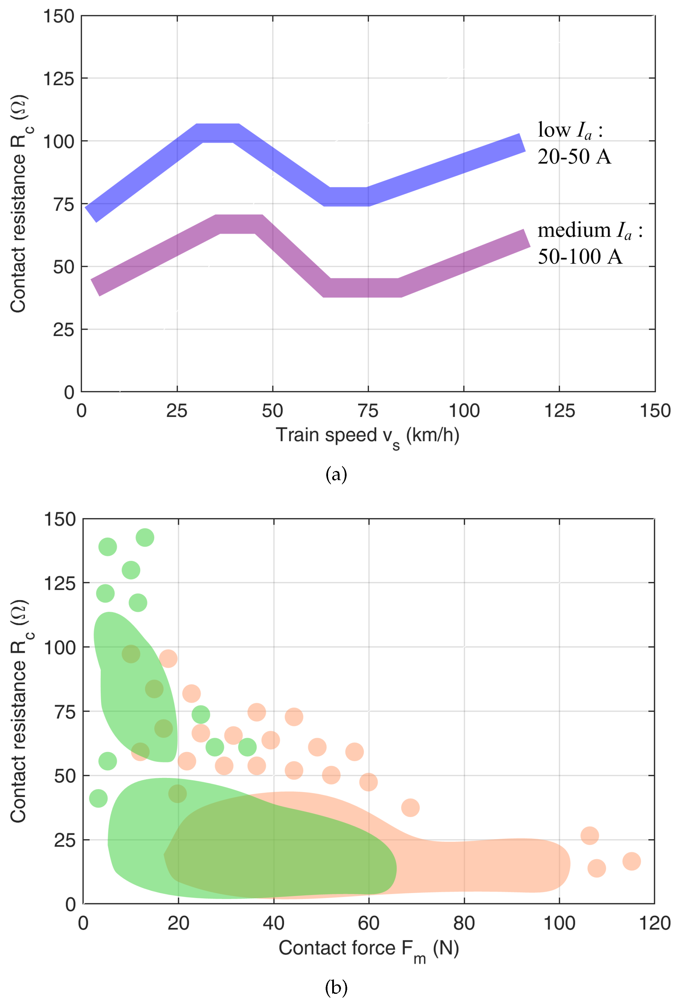
2.3. Electric Contact Resistance as a Function of Contact Force, Sliding Speed and Flowing Current

First of all it it is worth distinguishing between the static and the dynamic contact resistances (of electric nature) with obvious meaning and observing that the dynamic contact resistance can be made correspond to the electric arc resistance.
  • The static contact resistance R c s arises from the configuration of the stationary pantograph strip pressed against the contact wire and is subject to measurement under different intensity of the flowing current: the behaviour is inversely proportional to both the current intensity I a and the applied force F m with a larger variation in the low range of both, e.g., up to 20 A and 50 N to fix some reference values. A qualitative sketch is shown in Figure 4.
  • The dynamic contact resistance R c characterises all configurations with train motion; its behaviour versus current and force is more complex, basically considering that the purely vertical contact force of the static configuration is now skewed by a transverse friction in the direction of motion, with possibly minor components in the lateral direction due to the catenary staggering. The overall behaviour versus speed is an initial increase followed by a saddle with local reduction of the R c values and then a further increase; it is interesting to observe that this behaviour follows that of the friction coefficient. The exact shape depends of course on the applied force F m and the flowing current I a : as for the static contact resistance the most significant variations are observed at the lowest values, similar to the previously identified boundaries of 20 A and 50 N. A qualitative sketch is shown in Figure 4 distinguishing the dependency on train speed v and flowing current I a .
Figure 4. Static contact resistance vs. arc current I a for various contact force F m values: blue (about 20 N), pink (about 30 N to 50 N), light brown (about 50 N to 80 N), green (about 80 N to 120 N).
Energies 16 01465 g004
Several measurements were carried out in [93] keeping the sliding speed v s = 100 km / h and the arc current I a = 200 A in DC, showing almost doubled contact resistance values for the graphite strip than for the Kasperovski copper strip. Two interpolating expressions were derived for the contact resistance R c in Ω versus the loading contact force F m in N , but the original measured data are quite dispersed, as shown below.
R c ( Kasp ) = 0.013 + 0.09 e ( F m 14 ) / 11 R c ( graph ) = 0.015 + 0.18 e ( F m 4 ) / 7
An overall sketch of the results and of their distribution is shown in Figure 5. The curves in Figure 5a show the inversion phenomenon that creates a saddle at about 40 km/h to 70 km/h, after which there is again an increase with speed, but with a slightly lower slope [94]. The graphical representation in Figure 5b aims at showing the areas of clustered measured points (large coloured areas) indicating then where there are dispersed results (coloured circles).
It is worth underlining that the tests documented in the literature were carried out mostly at low-medium contact force values, in the order of some tens of N up to a hundred. With increasing speed the contact force increases and for high-speed trains values in the order of few hundreds N are common, as documented in [95], where the effect of pre-sag of the catenary and in general the dynamic behaviour of the contact force during a train run are shown. A significant oscillation of the contact force takes place, touching a minimum in the order of 50 N to 80 N every 50 m of simulated catenary (50 m corresponds to the separation of catenary masts). At each occurrence the electric contact resistance increases and there are the conditions for some arcing, e.g., as triggered by added train bouncing and wind force.
Starting from a different standpoint, that of very long arcs in static conditions, a simple formula is proposed in [59]:
R c = 2 2 π V a L I a
where V a and I a are the arc voltage and current (as defined previously in Section 2.2.1) and L is the electric arc length in m , which is intended as a large value for long arcs, so several times larger than the usual gap values at the sliding contact. It is worth noting that for long arcs the arc length L may be much longer than the electrode separation d.
A rapid comparison of this expression using the E a values considered in [59] (discussed in Section 2.2.1), taking L = 10 mm and an arc current I a = 100 A , the resulting arc resistance value is 0.11 Ω to 0.13 Ω , so among the worst values reported in Figure 5b. Reducing then the arc length to 5 mm, the predicted arc resistance would be half, so in the centre of the measured values, but going to shorter arc length values the effect of the surfaces and of the electric field distribution around the cathode cannot be ignored any longer.

2.4. Arc Duration and Electrode Erosion

2.4.1. Arc Duration and Its Dynamic Behaviour

The average arc lifetime (AAL) is an important measure of arc stability, taken as the time between arc initiation and self-extinction. Arc stability was identified in [14] as an important parameter for current collection, although we must underline that arcing occurs only at the detachment of pantograph and catenary, whereas the impression is that what was assumed at that time (47 years ago) was a more rigid current-collection system.
Arc stability at large current is confirmed by [14], where a 100 A arc is more tolerant to the variation of the inter-electrode gap (between 1 and 10 cm) than a 50 A arc, that shows a reduction of its AAL of two orders of magnitude. The Authors cogitate that the internal instability may be caused by increased susceptibility to self or external magnetic field or to the turbulence of the gas flow.
The cathode electrode shape is also highly important for the stabilisation of the electric arc, as explained quantitatively in [96], where the aligning force per-unit-length is calculated:
d F / d L = 10 6 I a 2 L sin α ( 1 cos α )
L being the arc length in mm , I a the arc current in A and α the arc inclination angle in degrees.
A small cathode electrode (like a pointed one) will exert a lower aligning force for which hollow cratered electrodes are usually preferred. The resulting AAL is generally ten times longer for the latter.
An overall picture of literature findings for the AAL dependency on the electrode geometry and arc current is reported in Figure 6.
As for the dynamic behaviour, arcs established between stationary electrodes possess their own speed of movement due to the interaction with the own magnetic field: values of arc velocity reported by Spink and Guile [97] for 9.6 mm brass electrodes are approximately linear with the arc current (about 80 m/s/kA for a 3.2 mm gap) and with a slope inversely proportional to the inter-electrode gap (longer arcs are slower, approximately linearly with their length).

2.4.2. Wear and Erosion of the Current Collection System

Although the focus of this work is on the electrical behavior of electric arcs for current collection in railway applications, selection of materials and technical solutions are heavily influenced by their behavior with respect to wear, that has a dramatic impact on reliability and safety of the collection system (pantograph or shoe) and of the overall ETS.
As well documented by Bucca and Collina [16] and further analyzed by Lee et al. [15], the normal wear rate (NWR) of the pantograph (expressed in volume of lost material per sliding distance, namely in mm 3 / km ) is a combination of the effect exerted by loading force and flowing current, including some experimentally adjusted parameters.
The original expression in [16] is:
N W R = k 1 1 2 1 + I a I 0 α F m F 0 β F m H + k 2 R c I a 2 H V ( 1 u ) + k 3 u V a I a V H m ρ
The overall NWR expression is reworked isolating several terms that indicate the contribution of the loading force F m alone ( N W R 1 ), of the flowing current I a alone ( N W R 2 ), of arcing erosion ( N W R 3 ) and the contribution of combined loading force and flowing current effect, distinguishing between synergy wear of flowing current to mechanical loading ( N W R 4 ) and viceversa of mechanical loading to flowing current ( N W R 5 ):
N W R 1 = k ˜ 1 F m F 0 β F m H
N W R 2 = 0.333 k 2 I a 2 H V ( 1 u )
N W R 3 = k 3 u V a I a V H m ρ
N W R 4 = k ˜ 1 α I a I 0 + α ( α 1 ) 2 I a I 0 2 α ( α 1 ) ( α 2 ) 6 I a I 0 3 +
N W R 5 = k 2 I a 2 H V ( 1 u ) ( 0.333 R c ) [ 1 e m ]
where:
F m is the total normal contact loading force in N ;
F 0 is the reference contact force in N (=90 for the results in [16]);
His the material hardness in MPa (=700 for copper);
H m is the fusion latent heat of the contact wire in kJ / kg ;
I 0 is the reference arc current in A (=500 for the results in [16]);
I a is the arc current in A ;
k 1 is an experimentally determined parameter related to the mechanical contact loading (adimensional, =22.4 for the results in [16]);
k 2 is an experimentally determined parameter related to the arc current (adimensional, =10.3 for the results in [16]);
k 3 is an experimentally determined parameter related to arc erosion (adimensional, =0.4 for the results in [16]);
α is the coefficient of dependence on the arc current (adimensional, =4.5 for the results in [16]);
β is the coefficient of dependence on the loading force (adimensional, =1.8 for the results in [16]);
R c is the contact resistance in Ω ;
uis the fraction of time for which the contact is lost (adimensional);
v s is the relative sliding velocity of the contact surfaces in m / s ;
v 0 is the reference velocity at the sliding contact in m / s (=44.4 for the results in [16]);
V a is the arc voltage, that is the potential difference between the contact wire and the current collector, in V ;
ρ is the mass density of copper in kg / m 3 (=8940).
The expressions reported above stem from least mean square fitting of the experimental results of [16] that are indeed quite dispersed, as previously shown for the electric contact resistance values in Figure 5.
Interestingly Lee et al. [15] observe that N W R 4 + N W R 5 is a negative term, that is reduces the effect of the two N W R 1 and N W R 2 terms, and is for this reason usually called “current lubrication”, adding some interpretation to what was stated in [16].
One last factor to consider for better understanding of wear is the power associated to the arc, that indeed depends on the arc voltage V a , in addition to the flowing arc current I a . The arc voltage has a complex dependency on the arc length, and on the arc current itself, the former related to the gap between the catenary and the contact strip (variable at each bounce and detachment) and the relative air flow speed (that depends in particular on the train speed) [93].

3. Electrical System Transient Response and Low-Frequency Conducted Emissions

Electrified railways, whether DC or AC, are characterised by a complex response that combines the natural transient response related to the physical length of the line sections [98] with the additional spurious responses caused by lumped loads, such as substations, rolling stock, and autotransformers, booster transformers, etc.
As a matter of fact, electric arcs are a wide-band excitation of the ETS transient response modes. The ignition of the electric arc corresponds to a step-wise voltage decrease or increase (depending on tractive or braking conditions) of the onboard internal line voltage downstream the pantograph. Such a step variation excites the rolling stock transient response and at a lesser extent the line transient response:
  • Rolling stock features a main response caused by the resonance of the onboard filter (DC rolling stock) or of the onboard transformer (AC rolling stock); whereas the DC onboard filter resonates around 10 Hz to 20 Hz [26,99], AC transformer resonances may be located at higher frequency, in the order of tens and hundreds of Hz, as they are caused by the stray inductance terms.
  • Line resonances for DC and AC railways are very similar, as they depend on the physical length and the per-unit-length parameters (not so different for lines with similar geometry) [100,101,102]; an exception is represented by the low-frequency resonance caused by the substation filter of DC railways studied extensively in [98,103,104].

3.1. Onboard and Substation Filters Excitation in DC Railways

The LC resonant filter located onboard DC rolling stock is quite relevant, as it is always provided although with different sizing and influences largely the system response [104].
The low-frequency transient response of the onboard filter manifests as an impressed current transient, as the filter inductance value is quite large, corresponding to several km of traction line inductance. Similarly, the traction power station (TPS) filter oscillation can be triggered by such a transient event if the locomotive happens to be not too far away: in this case the combined action can take the form of the oscillatory response shown in Figure 7. The slow onboard filter oscillation at about 20 Hz (corresponding to 50 ms) overlaps to the faster TPS filter oscillation, at about 120 Hz (corresponding to 8.33 ms, visible in the central portion left of 91.5 s). The appearance of TPS filter oscillatory response is a known byproduct of DC railways, as shown in [103], where a resonance peak of the pantograph impedance curve is visible slightly above 100 Hz and is clearly exposed to the excitation of an external source, such as the loco electric arc itself.
The relevance of such oscillatory responses is manifold. First of all, they are a source of low-frequency disturbance, not only for signalling circuits and devices connected to the track, but also for the control of the onboard braking chopper, causing undue energy dissipation [23]. The terms contributing to power losses are the arc itself (taking simply the integral of the voltage-current product), the triggered oscillations of onboard filter and the undue triggering of the rheostatic chopper (stabilising a catenary voltage excess that in reality is not there).
Filter oscillations then represent a bias for the components at higher frequency, possibly leading to out-of-scale issues, when for example measuring harmonics to assess disturbance to signalling. In fact, observing Figure 7, the otherwise small normal ripple around the DC line voltage of about 3800 V is masked by significant over and under voltages (peaking about 2000 V and 1400 V). The same for the pantograph current that was initially negative (braking condition) and then slowly return to the pristine value after the transient.
Finally, what reported as a power drive electromagnetic torque oscillation [25] brings indeed the signature of the onboard filter oscillation, as the reported curves have a 18 Hz resonant component. As discussed in the other case above, the onboard filter oscillation of a DC rolling stock has two significant drawbacks for the ETS electrical system: the capacitor voltage excursion may be significantly large disturbing the operation of the electrical systems onboard and the filter inductor behaves like a high-impedance current source, injecting its oscillating current back into the traction line by virtue of its larger inductance.
It is finally remarked that such oscillations occur mostly at low frequency, up to a hundred Hz , and that the damping of the traction supply circuit is negligible: the running rails in fact increase their longitudinal resistance because of skin effect only above it in the hundreds Hz and kHz range [105].

3.2. Onboard Transformer and Converter Excitation in AC Railways

The problem of electric arc effects on AC locomotive equipment was considered in [24], where a simple resistive-inductive circuit was used to observe the behaviour at the arc occurrence: the typical transient over-voltage at the current zero crossing is shown to have a sort of exponential decay with subsequent reduced amplitudes of the peaks and normal operation established after 3–4 periods; due to asymmetry of the positive and negative voltage peaks a DC component appears, as well as a 3rd harmonic, of p.u. amplitude 12% and 38%, respectively, for the studied example. What is observed is the triggering of the resonance of the input circuit, that for what reported is limited to the input transformer model: the resonance is not further discussed, but counting the ups and downs of the jagged voltage waveform the resonant frequency seems at about 4 kHz.
The simulated impact of pantograph arcing on a four-quadrant converter [106] identifies first of all the obvious effect of a temporary reduction of the DC link voltage (and of the AC voltage as well), as the arc voltage is in series to the pantograph input line. The corresponding current quantities are not visually affected, but their spectral analysis reveals a significant increase of the DC, 2nd and 3rd components of the AC current. In particular, the DC component increases as long as the arc duration 1/8 of the 50 Hz period, resulting in 20 A out of about 1 kA of nominal current, and this could create issues of transformer saturation. Similarly, the 100 Hz component increases by more than a factor of 2 passing from an arc duration of 1/8 to 1/2 of the 50 Hz period. In this case the most likely effect is the appearance of additional non-characteristic low-order harmonics.

3.3. Excitation of Line Resonances

ETSs, featuring long line sections interconnecting substations and loads, undergo the problem of resonant behaviour extended over several decades of frequency, whenever the poles of the transfer functions of ETS’s electrical quantities have low damping. Depending on the extension of the traction line, the first resonance may be located between some hundreds Hz and several kHz, inversely proportional to the length of sections between supply points. DC railways feature a shorter length of such sections (in the order of a dozen km or shorter for metros and tramways), whereas AC railways may be longer, ranging from 20 km to 40 km for 2 × 25 kV systems using Auto-Transformers (ATs) (with neutral or phase separation points to separate adjacent sections with different phase) to a hundred km for the other systems operated at 16.7, 50 and 60 Hz.
The theoretical model of line sections to predict resonances is based on a distributed parameters approach [107], as introduced long ago. Whereas AT-equipped railway lines have an asymmetric section termination with TPS at one side (with impedance Z T P S ) and neutral section at the other side (assimilated to an open-circuit condition), the other AC and DC lines have a symmetric termination with TPSs at both sides of each section, as observed in [102]. The expressions for the impedance seen by the moving train for the single TPS configuration ( Z 1 T P S ) and for TPSs at both ends ( Z 2 T P S ) are:
Z 1 T P S = Z c cosh γ ( D x ) Z T P S cosh γ x + Z c sinh γ x Z T P S sinh γ D + Z c cosh γ D
Z 2 T P S = Z c ( Z T P S cosh γ ( D x ) + Z c sinh γ ( D x ) ) ( Z T P S cosh γ x + Z c sinh γ x ) 2 Z c Z T P S cosh γ D + ( Z c 2 + Z T P S 2 ) sinh γ D
where x is the train position over the D length of the supply section, γ = ( r + j ω l ) ( j ω c ) is the propagation constant (neglecting as obvious transversal conductance terms), Z T P S is the TPS impedance and Z c = ( r + j ω l ) / ( j ω c ) is the characteristic impedance of the traction line.
The major source of resonance excitation is represented by the distortion of the rolling stock current absorbed through the pantograph (or sliding shoe, for some metros). Switching harmonics, as caused by pulse-width modulation schemes of the input converter typical of AC systems, extend with a significant amplitude up to a ten of kHz and able to excite the said line resonances. Electric arcs, as impulsive transients, have spectrum components of lower amplitude, although more extended in frequency, and represent a phenomenon common to both DC and AC railways. Resonances tend to reduce their factor of merit as the frequency increases, where line conductors and connected systems provide more damping. To this aim there are some phenomena that need to be included in any ETS model for a correct prevision of high-frequency resonant behaviour:
  • line conductors’ resistance is affected by skin effect [108], that depends not only on the magnetic characteristics of the conductor material (copper and copper alloys for supply conductors, magnetic steel for running rails [109]), but on the conductor cross section and shape (small conductors trigger skin effect at higher frequency);
  • proximity effect also plays a role [108], in particular when conductors are closely packed, as in the rolling stock input transformers, significantly increasing high-frequency damping and losses [110];
  • the soil is one of the conductive paths forming the return circuit, besides the running rails and aerial or buried earth conductors (in electric parallel through various connections and mutual leakage, represented by earth conductance terms).
As seen, the pantograph arc may be represented as an instantaneous voltage drop (a voltage source) appearing in series with the pantograph line and characterised by an internal resistance of moderate value, providing a first approximate static equivalent circuit. The dynamic behaviour is introduced by considering one of the electric arc models discussed in Section 2.2.
A direct interaction in an AC railway of the pantograph electric arc using a Mayr’s model was assumed in [111], modelling the railway line response based on the equivalent transmission line circuit described in [98]. However, modelling of the traction line is approximate indeed, as the measured (or simulated) response spectrum does not show any resonance phenomenon. Resonance of modern ETSs occurs over a broad frequency interval between some kHz and tens of kHz, with smaller value of the factor of merit as the frequency increases. In [26,112] in fact pantograph electric arcs in a DC railway trigger line resonances, to the extent that in [112] the transient response is used to identify the electrical parameters of the traction circuit itself: the results are good, but quality is affected by the limited sample rate available at the time of measurements for a resonance frequency in the order of 50 kHz. The resonance triggered by the electric arc [24] and previously commented as due to transformer resonant behaviour, could be as well the result of a combined line and transformer resonance.
A source able to trigger transient responses, strongly related to the pantograph electric arc, is the one associated with neutral (or phase separation) sections in AC ETSs. Each supply section is electrically separated and there is a procedure for the rolling stock to pass under such isolation phase changeover point, so that during passage the pantograph line of a long train does not risk the contemporary connection to two different supply sources with 120 phase rotation. A bold short circuit is prevented by lowering the pantograph and opening of the locomotive circuit breaker, that does not prevent the occurrence of dangerous events such as overvoltages caused by non-terminated transmission lines (either part of the neutral section or along the travelling train roof line, both approximately 200 m long) [113,114].

4. High-Frequency Transients and Radiated Emissions

Besides the excitation of the traction supply line circuit or large power devices (transformers and filters) in the low-frequency interval by their entire energy content of sub-ms duration, electric arcs are able to excite transient response at much higher frequency, by virtue of their faster turn-on time and intermittency.
A good evidence of two behaviours is provided in [115]: a “type-I arc” is reported with a more definite behaviour of arc initiation, ignition and extinction phases in the time domain and a spectral content mostly located at a few MHz ; the “type-II arc”, instead, is characterised by a jagged time-domain waveform with no definite phases and a spectral content moved to higher frequency, visibly in the tens of MHz . The amplitude of emissions is shown to be mostly influenced by speed, reporting an almost doubled amplitude at some characteristic frequencies, passing from 350 km/h to 450 km/h, where the latter speed is probably at the physical limit of the catenary system, that responds with more oscillations.
It is also interesting to observe that the 22 MHz frequency of relevant spectral components observed in [115] agrees with that reported by [38], discussed later in Section 6.3.
Considering then the propagation of the high-frequency components along the catenary system, we may say that the higher the frequency the shorter the propagation along the ETS, due to the larger resistive terms and associated losses [116]. It must be remembered that the focus is on the e.m. emissions originating from arc phenomena, and that not so many works have reported measurement results clearly related with such phenomena, rather than overall rolling stock and ETS e.m. emissions.
A pioneering work measuring radiated e.m. field in controlled conditions from stationary and rotating arcs in air and argon was carried out by Klapas et al. [117]. From a phenomenological and measurement standpoints conclusions may be summarised as:
  • results are expressed in dB μ V/m/MHz using a resolution bandwidth of 10 kHz and measuring distance for the antennas of 1 to 30 m; results are then expressed for a reference distance assuming a far-field radiation mode and that distance was selected as 1 m, invoking the now superseded standard MIL STD 462 [118];
  • there is no appreciable influence of the inter-electrode gap on the measured electric field strength;
  • arc at low current (below about 50 A) tend to be more unstable and produce slightly higher e.m. emissions; this was particularly evident at 100 MHz (about 5 dB between 50 and 100 A, and almost 10 dB between 100 and 200 A), whereas at 400 MHz the influence reduces to 4 dB between 50 and 100 A and 3 dB between 100 and 200 A;
  • frequent ignition and extinction of arcs increase the level of emissions, confirming that stable arcs (as observed at higher current intensity, and we will see in the absence of significant movement of the electrodes and wind) have lower emission profiles.
When carrying out measurements of e.m. field emissions by means of antennas, a second delicate point is ensuring that oscillating components appearing in the recorded signal are not introduced by one of the self-resonant modes of the antenna itself. This occurs for sure for narrowband antennas (such as those for radio communication systems) [119], whereas for broadband measuring antennas this should be a minor problem, although such antennas are (almost) never tested for their impulse response, nor this is declared as being verified or considered in scientific works.
A second systematic error in measuring e.m. field emissions of electric arcs is represented by the influence of the circuit feeding the electric arc itself, that in a real scenario includes the pantograph, the traction conductors and the train roof. Different setup geometries could impair reproducibility when attempting to compare results from different sources, e.g., spotting out the significance of some parameters, in particular speed.
Although the overall arc duration in real conditions may be in the order of hundreds of μ s or few ms , arc discharges are able to couple significant disturbance to receiving antennas nearby, where the tuning of such antennas is in the hundreds MHz or few GHz range and the separation distance exceeds several meters. This is discussed further in Section 5.
Recording of arc events may be challenging as a compromise between different exigencies. There is no “one size fits all” method, as each one in time or frequency domain has advantages and drawbacks.
  • A straight time-domain acquisition at high sample rate is unmanageable in terms of amount of data to store and subsequent post-processing; the small subset processed in [120] amounted to 25,700 records of about 2 MB each, over a 100 min travel time.
  • Arc transients last for a short time (the time duration T D ) and are separated by a long time interval (the repetition interval R I ), for which suitable triggering is able to capture and store only the relevant portions, reducing storage requirements and need to locate the transient within much longer recordings; nevertheless the R I information should be retained for its relevance to interference to radio communication system (RCS) (see Section 5).
  • Frequency domain equipment could be used to reduce the amount of data, set to max hold with a fast sweep or in zero span mode; the latter in fact would allow to follow the entire test run with multiple arcs, although it is applicable to RCS interference scenarios, having defined the centre frequency and the resolution bandwidth (RBW); the short T D values, however, require sufficiently large RBW values, larger than most of RCS bandwidth values; in the end even selecting 10 MHz may require some compensation for pulse desensitisation [121], sec. 9.2.13, that could be troublesome in the presence of sequences of arc pulses with variable duration.
Reference values of e.m. field emissions in clear relationship with electric arc phenomena are few. Two recent publications [122,123] provide two sets of data for measurements taken at high-speed AC railways, including a location with a neutral section. The values of the parameters a and b normalised to 10 m of distance are summarised in Table 2.
E ( 10 m ) = a + b log 10 ( f )
where f is expressed in MHz .
It appears that the two sets of results are different, but a comparison of the numeric values in the frequency interval of interest shows a moderate discrepancy, in the order of some dB. For the values provided by [122] the neutral section features higher values by about 20 dB than the normal line. As a recommendation new studies should compare to past published values, if they are supposed to apply to similar or identical conditions.

5. Radio Communication System (RCS) Disturbance

With the widespread use of radio communication services (RCSs) in ETSs for both safety and non-safety relevant applications, there has been a renewed research impetus for the modelling and prediction of interference, considering in particular the impulsive and random nature of electric arc emissions.
The commonly analysed RCSs for railway applications are:
  • The GSM-R is the bespoke GSM protocol adapted for railway signalling, using two reserved frequency bands at the margin of the commercial band, namely 873 MHz to 876 MHz and 918 MHz to 921 MHz for up-link and down-link, respectively [124]; the GSM-R is the data carrier for the European Train Control System protocol, implementing at the various levels voice and data transmission; the bandwidth of the single channel is 200 kHz and the used modulation is GMSK ensuring a data rate up to 172 kbps, quite slow if compared to the more modern LTE-R.
  • The Terrestrial Trunked Radio (TETRA) is a two-way mobile radio system extensively used for communication of maintenance staff, emergency coordination, fire squad and police within transportation systems of the metro and light railway transit type (railways operating often with the GSM-R); the emergency services operate over the 380 MHz to 385 MHz and 390 MHz to 395 MHz band, whereas civilian applications besides the remaining space between 385 MHz to 390 MHz and 395 MHz to 400 MHz are usually moved to 410 MHz to 470 MHz and around 900 MHz; the system also uses a TDMA assignment of time slots to users; the communication speed is limited to approximately 7 kbps per slot (half if IP encoding is used).
  • The LTE-R (Long-Term Evolution for railways) operates on a wide range of bands, from 450 MHz to 1.8 GHz, using a much larger bandwidth variable between 1 and 20 MHz and ensuring a quite high data rate that is not symmetric for the up-link (10 Mbps) and down-link (50 Mbps).
  • Wireless LAN (WLAN) systems are used instead on a local basis, for instance to implement train-to-wayside communication for both safety and non-safety related functions, such as CCTV, passenger information, train control (the Communications-Based Train Control, CBTC, is based on a WLAN protocol). Interference from commercial systems operating in the same 2.4 GHz and 5 GHz bands may occur (even as simply overloading causing a flood of packet rejections), so that there are implementations using a frequency offset of some hundreds MHz. Performances are those known for the commercial applications, not dissimilar from those of the LTE.
The study of the interference can be seen as a two-step process, where first a dataset of recorded representative waveforms or spectra is set up, and then it is fed to some simulation models of the victim RCS or just expressions synthesising RCS performance versus incoming noise (the latter corresponds to the known theory of the optimal receiver using the signal-to-noise ratio figure, SNR).
It must be remembered that when testing RCSs on site, especially at the highest operating frequencies, other interfering phenomena take place (and overlap to the effect of the electric arc impulsive disturbance), such as, not only multi-path fading (against which MIMO receivers are quite effective), but also Doppler shift (that unfortunately depends on the train speed as well) [125].

5.1. Electromagnetic Field Estimate at the RCS

The most direct approach to form the experimental dataset for a particular RCS is that of recording ETS noise (and in particular that originating from the electric arc) as captured by the RCS receiving antenna [119,126,127,128]. This approach has two drawbacks that hinder generalisation and re-use of data: as commented before, the impulse response of the antenna (usually a narrowband antenna tuned on the RCS frequency band [120]) appears within the recorded signals, casting some doubts on the reproducibility of the experiment with a different antenna for the same type of RCS; the signals measured through the RCS antenna cannot be use directly as an estimate of the e.m. field strength in that portion of space, unless the RCS antennas is characterised for its antenna factor and voltage standing wave ratio, as it is done for measuring antennas. These two negative points do not represent an insurmountable obstacle to the generalisation and re-use of a dataset for other RCSs, but require a complete characterisation of the RCS antenna.
General purpose EMC antennas have been used by other researchers [116,129], especially with the measuring station being located track-side and not on the train itself. Safety problems in fact dictate the use of roof installed antennas when doing tests onboard and discourage the use of larger EMC antennas, unless located inside the rolling stock [130]. As a note, the term “EMC antennas” identifies those antennas like loop, biconical and log-periodic commonly used for emissions tests in EMC. Nevertheless, results in [129] are expressed in dBm and generalisation of e.m. field strength values is not directly possible; however, the antennas are identified by their model numbers and reverse engineering of their antenna factors can be done offline.
For replication in the laboratory an ingenious approach is described in [131]: the pantograph arc is modelled by means of short L a , 0 = 30 mm wire and the GSM-R antenna is represented by a quarter-wavelength monopole; extensive numeric modelling was carried out to define the most relevant elements and parameters, considering for example the infinite catenary condition, so its extension beyond the metallic train roof and a way to terminate it (by two 200 Ω resistors at each end). The coupling coefficient S 21 between the electric arc and the GSM-R antenna was determined as 44.9 dB after some sensitivity analysis for variable length of the two catenary segments outside the train roof area. After validation by a scale model, the sensitivity to realistic conditions was assessed, by considering inclined arcing (as expected due to train movement at speed and corresponding to an arc length L a , i increasing beyond the L a , 0 nominal value), zig-zag arrangement of the catenary (staggering), variable height of catenary from train roof due to mechanical oscillations (implying a change of the length of the electric arc), and movement and folding of pantograph (again due to changes in the vertical height). The S 21 coefficient varied by 5 dB due to a 3 × change of L a , i = 3 L a , 0 and by ± 5 dB due to a factor of 3 below and above the nominal length L a , 0 .
Many instances of electric arcs were reproduced in the lab by means of a spinning wheel and the total power measured in a reverberating chamber under various conditions of rise time and resolution bandwidth of the spectrum analyser. The main problem in using the reverberating chamber is the trade-off between its Q-factor and time constant, the latter in the range of 0.12 μ s to 0.76 μ s, so always longer than the electric arc duration and rise-time used in the experiments. It is a sort of desensitisation of the reverberating chamber response, that is compensated experimentally by determining a corrective factor sending several simulated pulses by means of a transmitting antenna inside the chamber. The result is an apparent insensitivity of the spectrum analyser readings to the pulse duration and rise time, as if the method as an overall low-pass response compensated for the average value.
The received power was calculated then by applying directly the estimated S 21 coefficient and the electric field strength estimated by square rooting the result, demonstrating a practical approach. Of course, with more complex antennas a direct measurement of S 21 can be carried out, providing that the electric arc as radiating element is simulated by some kind of short conductor.
As commented in [132], to the aim of the validation of the results in [131], the highest estimated power level does not seem feasible with the operation of the GSM-R itself, if compared with its sensitivity of −85 dBm to −90 dBm, but the lowest discussed value is compatible with the frame error rate (FER) reported in [119,127].

5.2. Characteristics of the Electric Arc Transients and Interference to the RCS

Interference to RCSs is usually evaluated based on the signal-to-noise ratio (SNR) figure, that by virtue of the modelling of the electrical symbols sent over the physical channel, of the decision criteria and of the positive action of any error correcting code, give the resulting bit error rate (BER) and frame error rate (FER), up to an estimate of the availability and performance of the RCS function.
Many modern RCS of the narrowband type are based on a hybrid frequency- and time-based exploitation of the communication medium: the physical channel for transmission and reception is frequency coded, but the access to the medium is arranged in time slots, that is physical channels are defined with a Frequency Division Multiple Access (FDMA), but multiple subscribers share the same channel on a Time Division Multiple Access (TDMA) basis. This scheme is common to the GSM-R, TETRA, LTE-R etc. systems, where the narrowband nature facilitate not only transmission and reception, but also their protection by establishing limits of disturbance in the selected frequency bands at the standardisation level. Other RCSs may exploit instead broadband transmission methods, such as ultra-wideband (UWB) systems in use especially indoor for smart connection of personal devices and sensors.
The frequency-delimited physical channel simplifies the evaluation of interference using an approach based on channel power, that is in principle implemented with a zero-span reading centred on the channel carrier frequency and using a resolution bandwidth (RBW) to cover the channel extension. Large RBW values imply a fast spectrum analyser impulse response able to adequately follow the pulsed emissions dynamics. An opposite requisite is that of simulating the RCS bandwidth: consider for example the 300 kHz RBW value used by [133,134] to simulate the GSM-R bandwidth. The rise time of the intermediate frequency RBW filter is evaluated for various filter architectures in [121], sec. 9.2.5, encompassing Gaussian, analogue and digital filters, based on the few specifications provided by some manufacturers. Feasibility of sweep time values indicated by standards with respect to the selected RBW is then discussed in [132].
A first work to define the best measuring method for RCS interference assessment was carried out by [29], where one of the objectives was to rule out the quasi-peak detector as representative of the behaviour of modern RCS, promoting instead the use of the rms detector and noting a peculiar characteristic, that the output of the rms detector does not depend on the pulse width of the incoming repetitive pulsed noise. This holds if the pulse width is shorter than the RCS symbol rate, that does not always apply to our case: the mean pulse duration of about 20 ns reported in [119] is well below a GSM-R or TETRA symbol duration, but comparable to a LTE or WLAN symbol duration. Also for the repetition frequency (RF), the one observed in reality and discussed in Section 5.2.3 is at the limit of that assumed in [29] of about 10 kHz, after which the observed relationships for bit error probability and rms-measured signal-to-noise ratio lose their linearity and tend to saturate.

5.2.1. Amplitude Probability Distribution (APD)

Looking at the weakness of the swept frequency-domain method and achieving a better definition of the susceptibility of modern RCSs, the Amplitude Probability Distribution (APD) method is being studied extensively [31,33,135,136,137]. The APD detector quantifies the amount of time that the measured envelope r ( t ) of an incoming disturbing signal exceeds a given level [31], or, in other words, it is the complement to unity of the cumulative distribution function of the envelope.
The APD may equivalently be expressed in terms of the envelope energy (to compare with a threshold R) or, as customary for some RCS analyses, in terms of voltage, with a corresponding threshold, U calculated taking into account the receiver impedance Z and the bit duration T b , so to related energy and power.
A P D R = Pr r ( t ) R = Pr u ( t ) R Z T b = A P D U R Z T b
A basic relationship relating the probability density function f r of the envelope r to the APD is:
f r = d d r A P D r ( r )
being A P D r = 1 F r ( r ) by its own definition.
The APD is particularly well suited to quantify interference to a wide range of RCSs and resulting bit error probability. The APD method was shown to be applicable to some relevant digital RCS receivers [31,34,136] and could be equivalently transferred to other receivers and protocols, such as LTE [138].
The APD measurement can be achieved using a spectrum analyser (SA) with an envelope detector over the RCS band, as indicated in the CISPR 16-1-1 [139] (since this version usable also below 1 GHz), but a time-domain approach has more flexibility [33,140].
For use of a SA measurement, the resolution bandwidth (RBW) must be very similar to the RCS channel bandwidth, as transformation to other RBW values is not straightforward [31] and is considered more extensively in [141], where a method to change the APD values applicable to the class of pulse-modulated signals is discussed.
The APD implementation in time domain is described in [33], where an 8-bit digital sampling oscilloscope (DSO) is used and settings are optimised so that the DSO storage constraints can be met by choosing a short (channel 1) and a long (channel 2) time window, the former to capture the waveform of the single pulse and the latter to capture the duration and periodicity of the bursts of pulses. The pulse captured on channel 1, after a pre-selection band-pass filter to reject out-of-band components and the image signal, is passed through a mixer operating at the RCS frequency (indicated in the paper as f c ) with a chosen intermediate frequency and then to the RBW band-pass filter that has the same bandwidth of the RCS channel. This approach was chosen not only to strengthen the similarity with the SA approach, but also to make conveniently fast the transient response of the numeric RBW filter. A synthetic signal is then created using the filtered pulse captured on channel 1 and the information on burst duration and repetition obtained from channel 2. This signal is passed to the APD after a stage of envelope detection implemented with a Hilbert transform.
The APD is a flexible and comprehensive measure to use as performance index for RCS performance not only with steady Gaussian-noise-like sources, but also with impulsive noise sources, as discussed in the next section. However, regarding the applicability in general of the APD to complex communication protocols, it must be observed that the APD is a cumulative measure that does not indicate the original order in time of the envelope samples: there might be different noise waveforms producing the same APD. This is irrelevant if the receiver has no memory, as the bit decisions are statistically independent [31]; it is not for convolutional codes and when in general forward error correction is to be considered, as discussed below.

5.2.2. Bit Error Probability with Impulsive Noise Sources

It has been ascertained that the behaviour of the victim RCS in terms of bit error probability (BEP) and block (or frame) error probability (BLEP) is significantly affected by the type of received noise: the theory of the optimal receiver is well developed for incoherent noise, usually taken as an additive white Gaussian noise (AWGN); the railway electromagnetic environment is instead characterised by overlapped impulsive noise, as the one caused by electric arc emissions. From a practical standpoint, measuring the total disturbance average power within the RCS frequency band is a simple approach and is the extension of what has been normally done for a long time, by invoking the so called “Gaussian approximation” (GA). However, considering the waveform of the disturbance signal, and its impulsiveness in particular, RCS performance can be significantly affected with deviations from the expected behaviour under GA.
Since AWGN and impulsive sources overlap and their respective power may be higher or lower, a general model was recently shown in [35], considering a Middleton Type A mixed source. The original work dates back to about 25 years ago [142] and provides some additional demonstration of the basic theory. The total power σ 2 is the sum of the two power terms of the AWGN and impulsive source: σ 2 = σ G 2 + σ I 2 ; the ratio between the two is instead called Γ = σ G 2 / σ I 2 . To characterise the pulse density the impulse index A is used, that corresponds to the number of pulses per unit of time multiplied by the average duration of the single pulse: a low value of A implies higher impulsiveness with more rare separated impulses. The amplitude of the impulses is determined by the power σ I 2 , so having a large Γ value with a large A value means a large proportion of AWGN power, with several small impulses that become negligible (rather than one isolated large impulse, as a small A value would have implied).
The resulting BEP based on AWGN assumption using the signal-to-interference ratio (SIR) δ fails to give a good estimate, when the impulsive part of the impinging noise is relevant. For this reason it is proposed to correct this estimate by means of the impulsive correction factor (ICF).
SIR can be calculated by dividing the signal power P by the sum of all the noise power terms, provided that the AWGN assumption holds:
δ = P k = 1 K σ k 2 = P σ tot 2
where σ k 2 indicates the power of the k-th noise source and σ tot 2 is the total AWGN noise power. The ICF intervenes modifying the denominator of the SIR δ :
δ = P I C F σ tot 2
ICF is determined focusing on the most relevant noise source, that is assumed to be the dominant source of errors. The purpose of the ICF is to correct the SIR estimate for the presence of impulsive noise sources. A two-step process applicable to unequal power levels of the noise sources is described in [35]:
  • taking the power of each source σ k 2 and the total power σ tot 2 , the single ICFs for each source are adjusted for the relevance of the noise source:
    I C F adj , k = I C F k + 10 log 10 ( σ k 2 / σ tot 2 )
  • for the purpose of quantifying the final effect on BEP, under the assumption that the most intense source is the relevant one, the final ICF is determined taking the largest of the adjusted ones:
    I C F tot = max ( 0 , max k ( I C F adj , k ) )
The work, however, does not go in the detail of how determining the power of a single noise source, when they are all active at the same time and cannot be measured individually, posing a practical issue.
The advantage of the ICF is that it is a straightforward way to adjust the well-known calculation of BEP for impulsive noise sources. The ICF then can be estimated first, from BEP simulations (that we may say corresponds to its graphical interpretation), second, from “canonical” measurements using rms and average detectors readings, and, third, from APD measurements.

BEP Simulation

The BEP simulation is arranged considering a typical binary sequence modulated and sent over a channel affected by AWGN source to which then the impulsive source is overlapped. The comparison of the generated bit sequence with the sequence at the receiver after demodulation and decision at the receiver gives the number of erroneous bits, namely the bit error rate, made corresponding to the BEP.
A series of BEP vs. SNR curves are shown in [29,30] demonstrating two points: there is a difference of 7.5 dB on the horizontal SNR axis for BEP curves corresponding to different pulse repetition frequency f p , provided it is less than the symbol rate R S of the analysed modulation; curves plotted in the f p -SNR plane for different assigned BEP values are linear and parallel, provided that the BEP values are in the range of 10 3 to 10 6 , that corresponds to a reasonable operation, namely errors are not too frequent nor too rare.
The complete expression relating the energy per bit E b , the AWGN noise power density η G , the equivalent intensity of the impulsive source V I , rms and the pulse repetition rate compared to the symbol rate, is quite complex and was demonstrated in [29]. It is reported below for a two-symbol modulation like BPSK (Binary Phase Shift Keying):
B E P = 1 2 f p R S Q E b η G + 2 V I , rms η G f p cos ϕ + Q E b η G 2 V I , rms η G f p cos ϕ + 1 f p R S Q E b η G

Determination of BEP from APD

When using the APD as a form of statistic quantification of the noise intensity to estimate the resulting BEP, the most straightforward results are for an AWGN source and in [31] the method is extended to other types of noise sources. The key point is relating the amplitude r and phase ϕ of the incoming signal envelope to the decision moment of the receiver [31].
Pr { bit error | r , ϕ } = Q E b + r cos ( ϕ ) η
with η standing for a generic power spectral density and, in particular, that of the AWGN, so η = η G .
In this expression the APD comes into play for the estimation of f r as per (51). If the phase ϕ is assumed uniformly distributed over [ 0 , 2 π ] , then a general formula can be derived:
B E P = 1 2 π 0 2 π 0 Q E b + r cos ( ϕ ) η f r ( r ) d r d ϕ
In [31] the complexity is reduced by showing that by first calculating the conditional bit error probability depending on phase ϕ and then assuming a worst-case value of ϕ (that for the Binary Phase Shift Keying, BPSK, modulation is ϕ = π ), a general, yet simple, expression can be derived, relating the worst-case BEP to the APD calculated based on incoming power:
B E P m a x = A P D p ( E b )
BPSK is a simple binary modulation, on which all the other modulations are evaluated, deriving a slightly more complex expression, by introducing two parameters: α = T b / T s , the ratio of the time duration of a bit and of a symbol, and β , that weights the minimum distance between the points of the constellation of the specific modulation. A notation error can be seen in [31], for which α as defined here could be confused with another parameter, the ratio of pulse duration time and pulse repetition interval, that should instead receive the notation A = T p / R I . Matsumoto [32] one year later will comment on an inaccuracy of the original formula: the parameter α misses from the argument of the square root, that could be discovered only by analysing modulations with a number of symbols M > 2 .
B E P m a x = α A P D v ( β α P Z )

Determination of BEP from Measurements

The problem is approached by determining the ICF by measurements of the disturbance characteristics. A first approach appears in [30], where the ICF is estimated as the sum of an offset quantity (that depends on the type of modulation) and the impulsiveness ratio (IR) (that is determined by the said rms and average readings). To clarify, since the measurements are thought as channel or narrowband measurements, and not large sweeps over a wide frequency interval, the spectrum analyser is set to “zero span” and the right detector is selected, i.e., “rms” and “avg” detectors.
I C F = I C F offset + 3 4 I R
I R = 20 log 10 V rms V avg
The value of I C F offset is reported as 3 dB, 4 dB and 5 dB for MSK, BPSK and 64-QAM modulations, that are the most relevant for radio signalling applications in railways (with reference to the mentioned GSM-R and LTE-R systems).
Alternatively, a “peak” detector can be used and resulting readings applied as follows to estimate ICF [143]:
I C F = V p k ( Imp ) V p k ( AWGN )
where the difference is intended between the measurement of the impulsive source and an AWGN source of equal power, as assumed for the definition of ICF. This means that in principle an additional average power measurement of the impulsive source must be provided, so to set the local AWGN to the same power level.
A weak point of this approach is related to the random nature of the measured peak value for the AWGN, in that ideally for a long enough time it can be infinite and it is in general a random variable with an average value that is larger the longer the observation time (that is the larger the number of collected samples). The CISPR 16-1-1 [139] prescribes a 2 min measurement time specifically for the disturbance originating from microwave ovens; assuming a 1 MHz sampling suitable to track samples over a 100 kHz RCS bandwidth, the number of samples is in excess of 108, that provides a crest factor (ratio of peak to rms) of about 5.5. A general rule of thumb is to assume the crest factor equal to 6.

5.2.3. Influence of the Repetition Interval (RI)

Modern RCS have reduced their target BEP values due to the increased data rate and safety relevant systems may benefit from this to achieve high safety integrity levels (SIL), namely SIL4. Low BEP values are achieved with extensive use of complex message coding and error protection. For an exigency of optimisation, error protection codes make assumptions on the occurrence of noise as isolated spikes, bursts or repeated spikes and as a consequence control codes are spread over the message length. For this reason a parameter of great importance is the repetition frequency (RF) or repetition interval (RI) of the electric arc transients. A simple demonstration is the observation of an inaccessible WLAN (based on the 802.11n protocol) when reaching a peculiar 26 μ s RI value. while keeping the applied impulsive noise power constant [144].
RF (or RI) represents the hit density of the transients caused by pantograph arcing and it has been rarely evaluated in practice. The reason are the storage requirements and the large amount of data to post-process taking into account the necessary sampling rate and the relative low duty cycle of arc transients. This was the reason for the implementation of the time-domain APD detector using one fast and one slow channel, discussed in Section 5.2.1.
  • Statistics of the recorded transients are reported in [133], observing that the dispersion of RI values may be quite large and that isolated large values may bias the RI estimate, whilst being not relevant for the evaluation of interference, because they are much larger than the bit time (BT) of RCS like GSM-R; the observed distribution is a long-tail exponential, that reveals the problem of selecting a suitable threshold to calculate statistics like the mean value, standard deviation and inter-quartile range.
  • The influence of the repetition interval on the error probability referred to the single bit (BEP) and the entire frame (FEP) was experimentally evaluated in [145], where a complete test bench was also described for the assessment of GSM-R interference from controlled repetitive disturbance signals, such as recorded impulses; the results show a linearly decaying BEP with the RI value in a log-log scale, as expected, with a null FEP thanks to the positive action of the error correcting codes until the combination of low RI values and low SNR values reaches a threshold beyond which the discarded frames increase dramatically for small further reduction of RI and SNR (see Figure 8).
  • The repetition frequency has been put in relationship with the relative speed and with the supply voltage between the electrodes; in this case the inter-electrode gap is accurately set and the dependency on the two parameters (speed and voltage) was demonstrated with a significant repeatability in [8]; dispersion of RF values pertaining to the same speed or voltage values is negligible, whereas an approximately quadratic dependency on voltage and inverse quadratic on gap length is observed, as shown in Figure 9.
With a closer look at the dependency on the inter-electrode gap of Figure 9b for an applied voltage of approximately 40 kV (corresponding to the peak value of the 27.5 kV line voltage value), it can be observed that the resulting RI values are approximately distributed between 140 and 350 μ s, included in the wider spread observed in [133].
The reason for the many low RI occurrences reported in [133] under real line conditions may be twofold: first, most of the detachments are in the order of few mm, whereas the minimum gap applied in [8] is 5 mm and the used system is more rigid than a real catenary system; second, what is observed in [133] is the impulsive energy captured by the roof-top GSM-R antenna at about 900 MHz, so that arc intermittency (i.e., the fast on-off modulation of micro arcs) cannot be excluded, although not really visible if a broadband waveform is used, as in [8]. The hypotheses of intermittency or local instability is in line with the findings in [115], where the “type-II arc” is described as due to rapid oscillations at higher speed and consequential instability.
Figure 8. Dependency of the repetition frequency [145] on (a) BEP as a function of RI for different SNR values (the black thick curve corresponds to 0 dB); values missing for the lowest SNR and RI values refer to failed tests with loss of the communication link due to excessive errors. (b) BEP (black curves) and RBEP (plum curves) as a function of RI for different SNR values; dashed curves indicate SNR values of 0 dB and +3 dB with a 0 frame error rate (FER); solid curves are for SNR values of 2 dB and 3 dB and the non-null FER values are indicated by a number next to each dot. © 2012 IEEE. Reprinted, with permission, from [145].
Energies 16 01465 g008
Figure 9. Dependency of the repetition frequency [8] on (a) applied voltage, (b) inter-electrode gap. Reproduced with permission from [8]; published by MDPI, 2022.
Energies 16 01465 g009
The APD detector provides the distribution of the amplitude over the channel bandwidth, but in reality fails to characterise the time distribution, e.g., the repetition frequency values and their variability.
A joint time–frequency transform is able to retrieve the power spectrum distribution over time [119] with any kind of periodicity, but it is computationally unattractive, especially for long time intervals.
A more complete characterisation is possible if APD is complemented by the evaluation of the time distribution of interfering transients. In [146] the overall assessment is carried out by evaluating the APD for a single code block (assuming that all bits of a block are equally affected, that’s reasonable if Forward Error Correcting code and interleaving methods, such as turbo codes or low-density parity check codes, are used). This part is followed by the comparison of RI with the code block duration, evaluating a long-term error rate.
Geng et al. [146] introduce the pulse duration distribution (PDD) index in addition to the APD index for a thorough characterisation of interference caused by repetitive and time-varying impulsive disturbance. The proposed theoretical approach is able to cover all the three cases when the time interval between pulses (one instance of RI) is longer, approximately equal and shorter than the code block length; this allows the application of the method to slower and faster communication channels, passing from the older GSM-R with data rate of a hundred kbps to the newer LTE-R and WLAN systems with data rates in the order of a few tens Mbps. Results of simulations with RI between 10% and 100% of block time duration in [146] are consistent with those reported in the Figure 10 of [119].

5.3. Interference to External RCS

External radio systems may be assimilated to the RCSs operating in the ETS premises and the same methods may be used to assess performance reduction as caused by electromagnetic emissions. The larger distance ensures that disturbance intensity will be lower; in addition, most of the radio victims perform non-safety-relevant functions, that reduces the criticality of the assessment. Conversely, there are important functions, such as aviation radio assistance and in particular instrument landing system (ILS) services, that have emerged as possible victims and deserve a specific analysis.
As pointed out in [147], ETSs are a necessity to link airports with the cities they serve and can be found in close proximity to the airport services, despite the required electromagnetic protection zone of about 10 km radius around airports, taking the runway as the centre.
One of the first works to question the effect of an ETS located at 300 m from an airport runway [148] concluded that there was no active nor passive interference to the radio beacon. Conclusions were based on the assumption of free space propagation and an estimate of the source intensity based on previous measurements (the line subjected to analysis in fact was to be electrified in the near future). The electric field value taken as reference was, however, quite low, using an empirical formula of E = 61.46 10.46 log 10 ( f ) , with the frequency f expressed in MHz. The considered reference values are very low as the standard EN 50121-2 itself indicates limits about 30 dB μ V/m higher, although measured with a peak detector, whereas the values considered in [148] were quasi-peak. As a remark, the discrepancy between peak and quasi-peak readings may be variable depending on the nature of the measured disturbance, and assuming always the 20 dB reported in the CISPR 12 [149] does not have a solid ground and could bring in general to gross errors, as commented in [132], although for incoherent unmodulated pulses, as in the case of the electric arcs, a 10 dB to 15 dB difference is probably correct.
A specific case of a railway line with a discontinuity in the catenary causing persistent sparking at each train passage was analysed in [150]. The electric field emissions were measured at 10 m distance finding peak values much higher than those in [148] in the range 70 MHz to 200 MHz. The noise signal coupled into the aircraft ILS antenna was then estimated with a worst-case reasoning, assuming the lowest antenna factor. Such noise together with a simulated ILS signal (a carrier frequency of 75 MHz is modulated with the two ILS modulations at 90 Hz and 150 Hz) was fed to a real ILS receiver with a controlled signal-to-noise ratio. The results showed that the ILS input filter and the demodulation process are quite immune to external disturbance, with a receiver output (named “difference in depth modulation”) well within the International Civil Aviation Organisation limit of 0.5%.
Two new studies have been recently published both providing more experimental results of electric arc radiated emissions (already reported in Table 2) and evaluating the chances of interference to the ILS system. Xiao et al. conclude that the orientation of the beams of the airport radio system is relevant, that is detemrined by the aircraft position at the time of the communication depending on the function of the radio system. In this way the Marker Beacon function (operating at 75 MHz) would not be disturbed, whereas there are some constraints on separation distance to ensure some margin for the Localiser (operating at 108 MHz to 112 MHz) and Glide-Slope functions (operating at 328 MHz to 335 MHz). Tang et al. [151], instead, prefer to specify a speed reduction of the disturbing train, having noticed that electric arc emissions are proportional to speed.

6. Electric Arc Detection

The number of observed electric arcs is indicated as a direct index that assesses the quality of current collection in the standard EN 50367 [152], at its sec. 7.3, `Percentage of arcing’. Since long ago the detection of electric arc occurrence and the evaluation of its frequency have been recognised as a measure of the quality of current collection and as a diagnostic means of both the pantograph and the catenary.

6.1. Ultraviolet Emissions

Electric arcs can be detected by measuring the light emissions (mostly blue and ultraviolet), as experimentally investigated in particular about 20 years ago in Italy [40,41,153] and recently verified as part of the MyRailS project [154]. Electric arc emissions are well positioned in the blue and ultraviolet, as common to copper-copper and copper-graphite emissions: a first group of values ( 250.5 nm, 254.4 nm and 271.3 nm for Cu II) is located in the UV-C interval, whereas lines at 324.7 nm and 327.4 nm for Cu I are located midway between UV-B and UV-A, the remaining between 427.3 and 521.8 nm giving an intense blue colour [155]. The UV-C interval is particular attractive (in line with the choice made in [40]), because of the lower background noise of about 0.05   μ W/cm2 compared to an expected ten times higher electric arc emission.

6.2. Image Recognition

Image processing techniques applied to video streaming from roof-top cameras [43,44,156,157,158,159] have found significant interest for being non-intrusive and providing additional information for documenting the circumstances, besides exploiting a wide range of algorithms for image processing and recognition. In addition hardware has become particularly cheap and under continuous improvement. Many studies exploit visible light cameras and are based mainly on one of two basic image processing techniques: edge detection [42] or homogeneous intensity or colour areas [43].
An alternative light channel is used for instance in [44], by exploiting infrared images (in addition to images taken in normal visible light) with the objective of detecting the local temperature increase rather than the burst of light emission. An advantage of of infrared, as well as ultraviolet, image capturing is the relative insensitivity to variable daylight conditions. Besides then a straightforward thresholding of the intensity image map to locate the cluster of pixels corresponding to the heat or light spot, a convolutional neural network is used feeding it with images taken in various environmental light conditions, to further suppress the effects of scene lighting. The infrared channel provides useful information, but it is not exempt from failures: the authors show a few confounding cases of back light in a night scene taken for an arc event, as well as an arc occurring at the very end of the pantograph sliding arm is not detected (in this latter case we could say that such arcing should not occur because such extreme relative position of catenary and pantograph is hazardous.
In general such video based classification methods have significant accuracy. In particular, Huang et al. [44] underline the added value of information fusion, showing that classification based on visible light and infrared light taken separately achieves 89.0% and 94.5%, respectively, but information fusion of the two is able to achieve 97.5% overall accuracy.

6.3. Electromagnetic Emissions

Electromagnetic emissions of electric arc are not always a nuisance and an interesting application is that of detection and location of arc events, as recently proposed in [38,39] by exploiting electromagnetic radiated emissions:
  • Gao et al. [38] propose a Hilbert fractal antenna to measure the e.m. emissions of a laboratory electric arc setup, identifying frequencies (at 18 MHz and 60 MHz to 100 MHz in the present case) with significantly larger amplitude and characteristic of the arc phenomenon. The generality of such “characteristic frequencies” is demonstrated by showing that they are related to the arc specific resistance (the arc resistance normalised by its geometry) and the permittivity of air; even changing the inter-electrode gap the resonant characteristic frequency kept almost constant at the said 18 MHz. It is then proposed to exploit such arc signature for arc detection in real conditions.
  • Paoletti [39] solves elegantly the problem of the location of the pantograph arc by using two co-located shielded loop antennas, with their plane oriented at ± 45 deg with respect to the symmetry axis of the pantograph aligned with the train axis. The azimuthal angular position is found as the solution of a maximisation problem by taking the squared distance-weighted sum of the magnetic-field components measured by the two antennas. The search is one-dimensional, as it is known that the electric arc occurs at the pantograph contact strip. A remarkable accuracy of 8.6 mm was achieved in a real test at 400 km/h.
It can be acknowledged that methods based on e.m. field measurements may be more expensive in terms of hardware and might have some issues of installation on the roof top, whereas cameras have become quite small and robust.
More traditionally, the direct byproducts of the electric arc can be looked as conducted emissions, namely pantograph voltage and current [37,160,161,162]. Information is then extracted in various ways:
  • from classification of simple spectral properties (e.g., uncommon harmonic components) to projection in more complex spaces (such as using the S-transform or wavelets [160]) by considering voltage and current waveforms;
  • analysis of waveform features during arc occurrence, such as zero-current intervals and jagged voltage profile [37];
  • analysis of peculiar ETS responses, such as resonances, as caused by the electric arc seen as a discontinuity [161,162].
The use of the pantograph electrical quantities, although intrusive and in principle with a non negligible cost of the sensors and data acquisition, is again capturing interest for its possible combination with monitoring to prevent interference to track circuits [163,164] and, most of all, for optimisation of energy consumption onboard trains [154,165]. Simple algorithms with limited computational effort should be preferred for the possibility of embedding in the harmonic current monitor and energy meter devices (as evaluated for a similar task of detecting incipient traction line resonances in [102]).

7. Conclusions

The electrical and electromagnetic behaviour of electric arcs occurring at the sliding contact for current collection in railways has been discussed, comparing references spanning about 80 years.
The overall topic has been divided into: physical principles, arc modelling for static and dynamic behaviour, electrical effects at low frequency on the traction line and connected systems (such as substations and rolling stock), electromagnetic effects at higher frequency causing radiated electromagnetic emissions and disturbance to radio communication systems, and finally detection of arc occurrence.
Electric arc models and their applications have been thoroughly discussed in Section 2.2. Different formulas for static arc modelling have been proposed in a hundred years, for AC and DC phenomena, often customised on a set of experimental data and thus with quite a different behaviour, depending on the type of electrodes and their separation. Dynamic arc models were proposed initially about 80 years ago and have now reached a level of maturity that hardly other models will be found to improve the state of the art and be easily embedded in a circuit simulator. In general, they predict quite well the electric arc behaviour, although all necessitate a complex fine tuning of the numerous parameters to the specific experimental data, so that there is no general recipe to cover a wide range of arcs. It must be also recognised that even the electric arc phenomenon itself under constant conditions manifests a certain degree of variability in the order of a tens of %, for which model accuracy cannot be better. So, increasing the number of test cases and experimental results and improving the criteria for selection of parameters and fitting accuracy are two possible directions of research that would bring added value to the large number of available dynamic arc models.
The effect of the contact force, the sliding speed and the flowing current intensity on the contact resistance, as well as on the duration of the arc and wear of the contact surfaces, have been discussed in Section 2.3 and Section 2.4. As shown, general rules are difficult to derive not only for the intrinsic difficulty of the many interacting parameters, but also because the available datasets are quite few. However, it may be concluded that electric contact resistance is smaller for larger current intensity and larger contact force. Wear increases with flowing current intensity both due to self heating (term N W R 2 ) and arc erosion (term N W R 3 ), but the flowing current has also a beneficial “lubricating effect” in reducing wear when considered combined to mechanical loading (meaning that wear increases less than the estimate provided by the two terms N W R 2 and N W R 3 taken alone).
The response to electric arc excitation of ETS components (the catenary line and its natural resonant behaviour, the onboard transformer of AC rolling stock, as well as the resonant filters installed both onboard and at TPS of DC railways) is known in principle. It has been extensively analysed for some cases focusing on DC railways, providing insight in the non-linear behaviour of substation diodes, on the combination of concomitant transients at the substation and onboard and on the consequences, especially for energy efficiency, as discussed in Section 3. In particular for the operation of the braking chopper onboard and the impact on energy efficiency, the transient response of a DC vehicle should be well understood and taken into consideration. The effect on AC rolling stock (transformer resonance, appearance of a DC component and non-characteristic harmonics, etc.), instead, should receive more attention.
For radiated electromagnetic emissions (see Section 4), results have been provided since 40 years ago, as general characterisation of expected intensity, and more recently for analysing the spectral features of emissions (finding some characteristic frequencies) and modelling of electromagnetic coupling onto roof top antennas. With some personal experience of measurements of electric arc emissions, some considerations on the influence of the setup have been provided: e.g., resonance of the pantograph circuit, of the feeding circuit in lab, etc.
For the impact on RCSs there has been a significant work in the last 10–15 years, proceeding from modelling the effect on the bit error rate of impulsive noise sources and related measurements with spectrum analysers, to the derivation of specific performance indexes (such as the APD). The implementation in the electromagnetic compatibility standards, yet, is slow: the use of the APD originally proposed for frequencies above 1 GHz, is now allowed also below it, where most of the traditional railway RCSs (TETRA, GSM-R, LTE-R) operate.
The assessment of BEP in the presence of impulsive noise has been thoroughly discussed, providing a logic flow between the various approaches and ways to quantify BEP, as references span over more than 15 years and formulations are not always easy to relate one to the other, because e.g., of implicit assumptions, some ambiguity of notation and selection of parameters, etc. To this aim the most relevant characteristics are the RCS bandwidth and operating frequency, the energy per bit and the distance between symbols of the constellation diagram.
In view of the characteristics of digital RCS, such as the way they access the physical medium (time division multiplexing) and the message bits being distributed over time, another parameter that has a great importance is the arc pulses repetition interval: compared to the timing characteristic of the message block or frame duration and of the synchronisation for the access to the channel, specific values in the order of tens of μ s have demonstrated to be able to degrade significantly the RCS performance or even to block its operation, revealing thus a non-linear behaviour intrinsic to the RCS itself. For modern RCS with lower BEP targets and more complex message coding schemes understanding the effect of transient repetition and statistical distribution should be more thoroughly investigated, besides a solid background of APD extensive application and of setting of relevant frequency-domain detectors. From a practical viewpoint this would improve the methods for site validation, as well as the approach for SIL demonstration, taking into account more realistic disturbance scenarios.
The occurrence of electric arcs at the sliding contact is thus an important indicator of the quality of current collection and disturbance to RCSs and to the electric system in general. Electric arc detection is receiving much attention, with solutions that exploit several characteristics of the emissions: ultraviolet, infrared and visible light emissions, both detected by directive sensors as phototubes and recognised within a video stream by means of image processing and machine learning methods; conducted and radiated electromagnetic emissions, including in the former any detectable worsening of the quality of voltage and current waveforms. Image processing methods seem the most promising for being non-intrusive and useful for a general monitoring of the train roof area. Feature extraction from low-frequency conducted phenomena is also attracting attention for a possible implementation in the monitoring hardware already onboard, including a general verification of resonance and overvoltage conditions at the same time. Such methods should definitely be adopted to fulfil the requirements of counting the number of flashes for compliance with the quality parameter of the EN 50367 [152].
With the research impetus of the last 5–10 years that has seen both consolidation of older concepts and new research directions, it is expected that the forthcoming years will bring other new excellent findings, in terms in particular of widening the available experimental data, a more complete characterisation of the electromagnetic emissions (such as a confirmation of the “characteristic frequency”), new ideas and methods for detection and quantification of occurrence, and finally a thorough quantification of impulsive noise effects on modern radio protocols, comprising effects on the overall message block and the remedial action of error correcting codes.

Funding

This research received no external funding.

Institutional Review Board Statement

Not applicable.

Informed Consent Statement

Not applicable.

Conflicts of Interest

The authors declare no conflict of interest.

References

  1. Yang, Z.; Xu, P.; Wei, W.; Gao, G.; Zhou, N.; Wu, G. Influence of the Crosswind on the Pantograph Arcing Dynamics. IEEE Trans. Plasma Sci. 2020, 48, 2822–2830. [Google Scholar] [CrossRef]
  2. Wu, G.; Dong, K.; Xu, Z.; Xiao, S.; Wei, W.; Chen, H.; Li, J.; Huang, Z.; Li, J.; Gao, G.; et al. Pantograph–catenary electrical contact system of high-speed railways: Recent progress, challenges, and outlooks. Railw. Eng. Sci. 2022, 30, 437–467. [Google Scholar] [CrossRef]
  3. Wang, W.; Wu, G.; Gao, G.; Wang, B.; Zhou, L.; Cui, Y.; Liu, D. Experimental study of electrical characteristics on pantograph arcing. In Proceedings of the 2011 1st International Conference on Electric Power Equipment-Switching Technology, Xi’an, China, 23–27 October 2011. [Google Scholar] [CrossRef]
  4. Plesca, A.; Dumitrescu, C.; Calistru, C.N. Power collection system for electrical vehicles. In Proceedings of the 2016 IEEE 16th International Conference on Environment and Electrical Engineering (EEEIC), Florence, Italy, 7–10 June 2016. [Google Scholar] [CrossRef]
  5. Wu, G.; Wei, W.; Gao, G.; Wu, J.; Zhou, Y. Evolution of the electrical contact of dynamic pantograph–catenary system. J. Mod. Transp. 2016, 24, 132–138. [Google Scholar] [CrossRef]
  6. Wei, W.; Wu, J.; Gao, G.; Gu, Z.; Liu, X.; Zhu, G.; Wu, G. Study on Pantograph Arcing in a Laboratory Simulation System by High-Speed Photography. IEEE Trans. Plasma Sci. 2016, 44, 2438–2445. [Google Scholar] [CrossRef]
  7. Wu, G.; Wu, J.; Wei, W.; Zhou, Y.; Yang, Z.; Gao, G. Characteristics of the Sliding Electric Contact of Pantograph/Contact Wire Systems in Electric Railways. Energies 2017, 11, 17. [Google Scholar] [CrossRef]
  8. Jin, M.; Hu, M.; Li, H.; Yang, Y.; Liu, W.; Fang, Q.; Liu, S. Experimental Study on the Transient Disturbance Characteristics and Influence Factors of Pantograph–Catenary Discharge. Energies 2022, 15, 5959. [Google Scholar] [CrossRef]
  9. Kubo, S.; Kato, K. Effect of arc discharge on the wear rate and wear mode transition of a copper-impregnated metallized carbon contact strip sliding against a copper disk. Tribol. Int. 1999, 32, 367–378. [Google Scholar] [CrossRef]
  10. Ding, T.; Chen, G.X.; Bu, J.; Zhang, W.H. Effect of temperature and arc discharge on friction and wear behaviours of carbon strip/copper contact wire in pantograph–catenary systems. Wear 2011, 271, 1629–1636. [Google Scholar] [CrossRef]
  11. Yang, H.; Li, C.; Liu, Y.; Fu, L.; Jiang, G.; Cui, X.; Hu, B.; Wang, K. Study on the delamination wear and its influence on the conductivity of the carbon contact strip in pantograph-catenary system under high-speed current-carrying condition. Wear 2021, 477, 203823. [Google Scholar] [CrossRef]
  12. Zhang, Y.; Li, C.; Pang, X.; Song, C.; Ni, F.; Zhang, Y. Evolution processes of the tribological properties in pantograph/catenary system affected by dynamic contact force during current-carrying sliding. Wear 2021, 477, 203809. [Google Scholar] [CrossRef]
  13. Li, S.; Yang, X.; Kang, Y.; Li, Z.; Li, H. Progress on Current-Carry Friction and Wear: An Overview from Measurements to Mechanism. Coatings 2022, 12, 1345. [Google Scholar] [CrossRef]
  14. Klapas, D.; Hackam, R.; Beanson, F. Electric arc power collection for high-speed trains. Proc. IEEE 1976, 64, 1699–1715. [Google Scholar] [CrossRef]
  15. Lee, C.Y.; Huang, C.H.; Lin, H.E.; Lin, J.Y.; Yu, S.P.; Yang, Y.L.; Huang, H.H. Modelling on the synergy of mechanical and electrical wear in a current line/catenary-pantograph system. J. Phys. Conf. Ser. 2022, 2345, 012001. [Google Scholar] [CrossRef]
  16. Bucca, G.; Collina, A. Electromechanical interaction between carbon-based pantograph strip and copper contact wire: A heuristic wear model. Tribol. Int. 2015, 92, 47–56. [Google Scholar] [CrossRef]
  17. Chen, Z.; Liu, P.; Verhoeven, J.; Gibson, E. Electrotribological behavior of Cu-15 vol.% Cr in situ composites under dry sliding. Wear 1997, 203–204, 28–35. [Google Scholar] [CrossRef]
  18. Wang, Y.; Li, J.; Yan, Y.; Qiao, L. Effect of electrical current on tribological behavior of copper-impregnated metallized carbon against a Cu–Cr–Zr alloy. Tribol. Int. 2012, 50, 26–34. [Google Scholar] [CrossRef]
  19. Midya, S.; Bormann, D.; Schutte, T.; Thottappillil, R. Pantograph Arcing in Electrified Railways—Mechanism and Influence of Various Parameters—Part I: With DC Traction Power Supply. IEEE Trans. Power Deliv. 2009, 24, 1931–1939. [Google Scholar] [CrossRef]
  20. Midya, S.; Bormann, D.; Schutte, T.; Thottappillil, R. Pantograph Arcing in Electrified Railways—Mechanism and Influence of Various Parameters—Part II: With AC Traction Power Supply. IEEE Trans. Power Deliv. 2009, 24, 1940–1950. [Google Scholar] [CrossRef]
  21. Mariscotti, A. Characterization of Power Quality transient phenomena of DC railway traction supply. ACTA IMEKO 2012, 1, 26. [Google Scholar] [CrossRef]
  22. Crotti, G.; Giordano, D.; Roccato, P.; Femine, A.D.; Gallo, D.; Landi, C.; Luiso, M.; Mariscotti, A. Pantograph-to-OHL Arc: Conducted Effects in DC Railway Supply System. In Proceedings of the 2018 IEEE 9th International Workshop on Applied Measurements for Power Systems (AMPS), Bologna, Italy, 26–28 September 2018. [Google Scholar] [CrossRef]
  23. Mariscotti, A.; Giordano, D.; Femine, A.D.; Gallo, D.; Signorino, D. How Pantograph Electric Arcs affect Energy Efficiency in DC Railway Vehicles. In Proceedings of the 2020 IEEE Vehicle Power and Propulsion Conference (VPPC), Gijon, Spain, 18 November–16 December 2020. [Google Scholar] [CrossRef]
  24. Li, T.; Wu, G.; Zhou, L.; Gao, G.; Wang, W.; Wang, B.; Liu, D.; Li, D. Pantograph Arcing Impact on Locomotive Equipments. In Proceedings of the 2011 IEEE 57th Holm Conference on Electrical Contacts (Holm), Minneapolis, MN, USA, 11–14 September 2011. [Google Scholar] [CrossRef]
  25. Pefia-Eguiluz, R. Pantograph detachment perturbation on a railway traction system. In Proceedings of the 8th International Conference on Power Electronics and Variable Speed Drives, Minneapolis, MN, USA, 11–14 September 2011. [Google Scholar] [CrossRef]
  26. Mariscotti, A.; Giordano, D. Experimental Characterization of Pantograph Arcs and Transient Conducted Phenomena in DC Railways. ACTA IMEKO 2020, 9, 10. [Google Scholar] [CrossRef]
  27. Midya, S.; Bormann, D.; Mazloom, Z.; Schutte, T.; Thottappillil, R. Conducted and radiated emission from pantograph arcing in AC traction system. In Proceedings of the 2009 IEEE Power & Energy Society General Meeting, Calgary, AB, Canada, 2 October 2009. [Google Scholar] [CrossRef]
  28. Guo, F.; Wang, Z.; Zheng, Z.; Zhang, J.; Wang, H. Electromagnetic noise of pantograph arc under low current conditions. Int. J. Appl. Electromagn. Mech. 2017, 53, 397–408. [Google Scholar] [CrossRef]
  29. Stenumgaard, P. Using the root-mean-square detector for weighting of disturbances according to its effect on digital communication services. IEEE Trans. Electromagn. Compat. 2000, 42, 368–375. [Google Scholar] [CrossRef]
  30. Stenumgaard, P. A simple impulsiveness correction factor for control of electromagnetic interference in dynamic wireless applications. IEEE Commun. Lett. 2006, 10, 147–149. [Google Scholar] [CrossRef]
  31. Wiklundh, K. Relation Between the Amplitude Probability Distribution of an Interfering Signal and its Impact on Digital Radio Receivers. IEEE Trans. Electromagn. Compat. 2006, 48, 537–544. [Google Scholar] [CrossRef]
  32. Matsumoto, Y. On the Relation Between the Amplitude Probability Distribution of Noise and Bit Error Probability. IEEE Trans. Electromagn. Compat. 2007, 49, 940–941. [Google Scholar] [CrossRef]
  33. Pous, M.; Silva, F. APD radiated transient measurements produced by electric sparks employing time-domain captures. In Proceedings of the 2014 International Symposium on Electromagnetic Compatibility, Gothenburg, Sweden, 1–4 September 2014. [Google Scholar] [CrossRef]
  34. Pous, M.; Azpurua, M.A.; Silva, F. Measurement and Evaluation Techniques to Estimate the Degradation Produced by the Radiated Transients Interference to the GSM System. IEEE Trans. Electromagn. Compat. 2015, 57, 1382–1390. [Google Scholar] [CrossRef]
  35. Tengstrand, S.O.; Axell, E.; Fors, K.; Linder, S.; Wiklundh, K. Efficient evaluation of communication system performance in complex interference situations. In Proceedings of the 2017 International Symposium on Electromagnetic Compatibility—EMC EUROPE, Angers, France, 4–7 September 2017. [Google Scholar] [CrossRef]
  36. Eliardsson, P.; Axell, E.; Komulainen, A.; Wiklundh, K.; Tengstrand, S.O. A Practical Method for BEP Estimation of Convolutional Coding in Impulse Noise Environments. In Proceedings of the IEEE Military Communications Conference (MILCOM), Norfolk, VA, USA, 12–14 November 2019. [Google Scholar] [CrossRef]
  37. Mochizuka, H.; Kusumi, S.; Nagasawa, H. New Detection Method for Contact Loss of Pantograph. Q. Rep. RTRI 2000, 41, 173–176. [Google Scholar] [CrossRef]
  38. Gao, G.; Yan, X.; Yang, Z.; Wei, W.; Hu, Y.; Wu, G. Pantograph–Catenary Arcing Detection Based on Electromagnetic Radiation. IEEE Trans. Electromagn. Compat. 2019, 61, 983–989. [Google Scholar] [CrossRef]
  39. Paoletti, U. Direction Finding Techniques in Reactive Near Field of Impulsive Electromagnetic Noise Source Aiming at Pantograph Arcing Localization. IEEE Sens. J. 2019, 19, 4193–4200. [Google Scholar] [CrossRef]
  40. Bruno, O.; Landi, A.; Papi, M.; Sani, L. Phototube sensor for monitoring the quality of current collection on overhead electrified railways. Proc. Inst. Mech. Eng. Part F J. Rail Rapid Transit 2001, 215, 231–241. [Google Scholar] [CrossRef]
  41. Barmada, S.; Raugi, M.; Tucci, M.; Romano, F. Arc detection in pantograph-catenary systems by the use of support vector machines-based classification. IET Electr. Syst. Transp. 2014, 4, 45–52. [Google Scholar] [CrossRef]
  42. Aydin, I.; Karaköse, M.; Akin, E. A new contactless fault diagnosis approach for pantograph-catenary system. In Proceedings of the 15th International Conference MECHATRONIKA, Prague, Czech Republic, 5–7 December 2012. [Google Scholar]
  43. Huang, S.; Yu, L.; Zhang, F.; Zhu, W.; Guo, Q. Cluster Analysis Based Arc Detection in Pantograph-Catenary System. J. Adv. Transp. 2018, 2018, 1–12. [Google Scholar] [CrossRef]
  44. Huang, S.; Chen, W.; Sun, B.; Tao, T.; Yang, L. Arc Detection and Recognition in the Pantograph-Catenary System Based on Multi-Information Fusion. Transp. Res. Rec. J. Transp. Res. Board 2020, 2674, 229–240. [Google Scholar] [CrossRef]
  45. Steinmetz, C.P. Transformation of Electric Power into Light. Trans. Am. Inst. Electr. Eng. 1906, XXV, 789–813. [Google Scholar] [CrossRef]
  46. Slepian, J. Extinction of a Long A-C Arc. Trans. Am. Inst. Electr. Eng. 1930, 49, 421–430. [Google Scholar] [CrossRef]
  47. Browne, T.E. Extinction of Short A-C Arcs. Trans. Am. Inst. Electr. Eng. 1931, 50, 1461–1464. [Google Scholar] [CrossRef]
  48. Cassie, A.M. Theorie Nouvelle des Arcs de Rupture et de la Rigidité des Circuits. CIGRE 1939, 102, 588–608. [Google Scholar]
  49. Slepian, J.; Browne, T.E. Photographic study of A-C arcs in flowing liquids. Electr. Eng. 1941, 60, 823–828. [Google Scholar] [CrossRef]
  50. Slepian, J. Displacement and diffusion in fluid-flow arc extinction. Electr. Eng. 1941, 60, 162–167. [Google Scholar] [CrossRef]
  51. Mayr, O. Beitrage zur theorie des statischen und des dynamischen lichtbogens. Electr. Eng. Arch. Elektrotech. 1943, 37, 588–608. [Google Scholar] [CrossRef]
  52. Browne, T.E. A Study of A-C Arc Behavior Near Current Zero by Means or Mathematical Models. Trans. Am. Inst. Electr. Eng. 1948, 67, 141–153. [Google Scholar] [CrossRef]
  53. Schwarz, J. Dynamisches verhalten eines gasbeblasenen, turbulenzbestimmten schaltlichtbogens. ETZ-Archiv 1971, 92, 389–391. [Google Scholar]
  54. Habedank, U. On the Mathematical Description of Arc Behaviour in the Vicinity of Current Zero. ETZ-Archiv 1988, 10, 339–343. [Google Scholar]
  55. Mauriello, A.; Clarke, J. Measurement and Analysis of Radiated Electromagnetic Emissions from Rail-Transit Vehicles. IEEE Trans. Electromagn. Compat. 1983, EMC-25, 405–411. [Google Scholar] [CrossRef]
  56. Ammerman, R.F.; Sen, P. Modeling High-Current Electrical Arcs: A Volt-Ampere Characteristic Perspective for AC and DC Systems. In Proceedings of the 2007 39th North American Power Symposium, Las Cruces, NM, USA, 30 September–2 October 2007. [Google Scholar] [CrossRef]
  57. Wright, D.; Delmont, P.; Torrilhon, M. Modeling of electric arcs: A study of the non-convective case with strong coupling. J. Plasma Phys. 2013, 79, 699–713. [Google Scholar] [CrossRef]
  58. Li, J.; Yuan, H.; Xu, M.; Tian, F.; Wang, Z.; Ren, J. Research on Improved Schwarz Arc Model Considering Dynamic Arc Length. J. Electr. Eng. Technol. 2022. [Google Scholar] [CrossRef]
  59. Terzija, V.; Koglin, H.J. On the Modeling of Long Arc in Still Air and Arc Resistance Calculation. IEEE Trans. Power Deliv. 2004, 19, 1012–1017. [Google Scholar] [CrossRef]
  60. Goda, Y.; Iwata, M.; Ikeda, K.; Tanaka, S. Arc voltage characteristics of high current fault arcs in long gaps. IEEE Trans. Power Deliv. 2000, 15, 791–795. [Google Scholar] [CrossRef]
  61. Nottingham, W.B. A New Equation for the Static Characteristic of the Normal Electric Arc. Trans. Am. Inst. Electr. Eng. 1923, XLII, 302–310. [Google Scholar] [CrossRef]
  62. Browne, T.E. The Electric Arc as a Circuit Element. J. Electrochem. Soc. 1955, 102, 27. [Google Scholar] [CrossRef]
  63. Fisher, L.E. Resistance of Low-Voltage AC Arcs. IEEE Trans. Ind. Gen. Appl. 1970, IGA-6, 607–616. [Google Scholar] [CrossRef]
  64. Stokes, A.D.; Oppenlander, W.T. Electric arcs in open air. J. Phys. Appl. Phys. 1991, 24, 26–35. [Google Scholar] [CrossRef]
  65. Van, A.R.; Warrington, C. Reactance relays negligibly affected by arc impedance. Electr. World 1931, 1931, 502–505. [Google Scholar]
  66. Andrade, V.D.; Sorrentino, E. Typical expected values of the fault resistance in power systems. In Proceedings of the 2010 IEEE/PES Transmission and Distribution Conference and Exposition: Latin America, Sao Paulo, Brazi, 8–10 November 2010. [Google Scholar] [CrossRef]
  67. Pessoa, F.P.; Acosta, J.S.; Tavares, M.C. Parameter estimation of DC black-box arc models using genetic algorithms. Electr. Power Syst. Res. 2021, 198, 107322. [Google Scholar] [CrossRef]
  68. Trelles, J.P.; Chazelas, C.; Vardelle, A.; Heberlein, J.V.R. Arc Plasma Torch Modeling. J. Therm. Spray Technol. 2009, 18, 728–752. [Google Scholar] [CrossRef]
  69. Wu, Z.; Wu, G.; Dapino, M.; Pan, L.; Ni, K. Model for Variable-Length Electrical Arc Plasmas Under AC Conditions. IEEE Trans. Plasma Sci. 2015, 43, 2730–2737. [Google Scholar] [CrossRef]
  70. Sawicki, A.; Haltof, M. Mathematical models of electric arc with variable plasma column length used for simulations of processes in gliding arc plasmatrons. Prz. Elektrotech. 2016, 1, 195–198. [Google Scholar] [CrossRef]
  71. Sawicki, A. Problems of modeling an electrical arc with variable geometric dimensions. Prz. Elektrotech. 2013, 89, 270–275. [Google Scholar]
  72. Park, K.H.; Lee, H.Y.; Asif, M.; Lee, B.W. Parameter identification of dc black-box arc model using non-linear least squares. J. Eng. 2018, 2019, 2202–2206. [Google Scholar] [CrossRef]
  73. Jalil, M.; Samet, H.; Ghanbari, T. Time-Variant Schwarz Based Model for DC Series Arc Fault Modeling in Photovoltaic Systems. IEEE J. Photovolt. 2022, 12, 1078–1089. [Google Scholar] [CrossRef]
  74. Guardado, J.; Maximov, S.; Melgoza, E.; Naredo, J.; Moreno, P. An Improved Arc Model Before Current Zero Based on the Combined Mayr and Cassie Arc Models. IEEE Trans. Power Deliv. 2005, 20, 138–142. [Google Scholar] [CrossRef]
  75. Habedank, U. Application of a new arc model for the evaluation of short-circuit breaking tests. IEEE Trans. Power Deliv. 1993, 8, 1921–1925. [Google Scholar] [CrossRef]
  76. Tseng, K.J.; Wang, Y.; Vilathgamuwa, D. An experimentally verified hybrid Cassie-Mayr electric arc model for power electronics simulations. IEEE Trans. Power Electron. 1997, 12, 429–436. [Google Scholar] [CrossRef]
  77. Dai, J.; Hao, R.; You, X.; Sun, H.; Huang, X.; Li, Y. Modeling of plasma arc for the high power arc heater in MATLAB. In Proceedings of the 2010 5th IEEE Conference on Industrial Electronics and Applications, Taichung, Taiwan, 15–17 June 2010. [Google Scholar] [CrossRef]
  78. Schavemaker, P.; van der Slui, L. An improved Mayr-type arc model based on current-zero measurements [circuit breakers]. IEEE Trans. Power Deliv. 2000, 15, 580–584. [Google Scholar] [CrossRef]
  79. Smeets, R.; Kertesz, V. Evaluation of high-voltage circuit breaker performance with a new validated arc model. IEE Proc. Gener. Transm. Distrib. 2000, 147, 121. [Google Scholar] [CrossRef]
  80. Rashtchi, V.; Lotfi, A.; Mousavi, A. Identification of KEMA arc model parameters in high voltage circuit breaker by using of genetic algorithm. In Proceedings of the 2008 IEEE 2nd International Power and Energy Conference, Johor Bahru, Malaysia, 1–3 December 2008. [Google Scholar] [CrossRef]
  81. Khakpour, A.; Franke, S.; Uhrlandt, D.; Gorchakov, S.; Methling, R.P. Electrical Arc Model Based on Physical Parameters and Power Calculation. IEEE Trans. Plasma Sci. 2015, 43, 2721–2729. [Google Scholar] [CrossRef]
  82. Khakpour, A.; Franke, S.; Gortschakow, S.; Uhrlandt, D.; Methling, R.; Weltmann, K.D. An Improved Arc Model Based on the Arc Diameter. IEEE Trans. Power Deliv. 2016, 31, 1335–1341. [Google Scholar] [CrossRef]
  83. Wang, Y.; Liu, Z.; Mu, X.; Huang, K.; Wang, H.; Gao, S. An Extended Habedank’s Equation-Based EMTP Model of Pantograph Arcing Considering Pantograph-Catenary Interactions and Train Speeds. IEEE Trans. Power Deliv. 2016, 31, 1186–1194. [Google Scholar] [CrossRef]
  84. Amirdehi, S.; Trajin, B.; Vidal, P.E.; Vally, J.; Colin, D.; Rotella, F. Pantographs bounce modelling for the simulation of railway systems. In Proceedings of the PCIM Europe 2019—International Exhibition and Conference for Power Electronics, Intelligent Motion, Renewable Energy and Energy Management, Nürnberg, Deutschland, 7–9 May 2019. [Google Scholar]
  85. Li, X.; Pan, C.; Luo, D.; Sun, Y. Series DC Arc Simulation of Photovoltaic System Based on Habedank Model. Energies 2020, 13, 1416. [Google Scholar] [CrossRef]
  86. Ju, M.; Wang, L. Arc fault modeling and simulation in DC system based on Habedank model. In Proceedings of the 2016 Prognostics and System Health Management Conference (PHM-Chengdu), Chengdu, China, 19–21 October 2016. [Google Scholar] [CrossRef]
  87. He, J.; Wang, K.; Li, J. Application of an Improved Mayr-Type Arc Model in Pyro-Breakers Utilized in Superconducting Fusion Facilities. Energies 2021, 14, 4383. [Google Scholar] [CrossRef]
  88. Xu, Y.; Guo, M.; Chen, B.; Yang, G. Modeling and simulation analysis of arc in distribution network. Dianli Xitong Baohu Yu Kongzhi/Power Syst. Prot. Control 2015, 43, 57–64. [Google Scholar]
  89. Berger, S. Modell zur Berechnung des Dynamischenelektrischen Verhaltens rasch Verlängerter Lichtbögen. Ph.D. Thesis, ETH Zürich, Zürich, Switzerland, 2009. [Google Scholar]
  90. Sawicki, A. Modele łuku elektrycznego o sterowanej długości. Wiad. Elektrotech. 2012, 7, 15–19. [Google Scholar]
  91. Sawicki, A. Modelowanie łuku elektrycznego o zmiennychrozmiarach geometrycznych. Zesz. Nauk. Politech. 2012, 124, 202–214. [Google Scholar]
  92. Yuan, L.; Sun, L.; Wu, H. Simulation of Fault Arc Using Conventional Arc Models. Energy Power Eng. 2013, 5, 833–837. [Google Scholar] [CrossRef]
  93. Bucca, G.; Collina, A.; Manigrasso, R.; Mapelli, F.; Tarsitano, D. Analysis of electrical interferences related to the current collection quality in pantograph–catenary interaction. Proc. Inst. Mech. Eng. Part F J. Rail Rapid Transit 2011, 225, 483–500. [Google Scholar] [CrossRef]
  94. Wu, G.; Gao, G.; Wei, W.; Yang, Z. The Electrical Contact of the Pantograph-Catenary System—Theory and Application; Springer: Berlin, Germany, 2019. [Google Scholar] [CrossRef]
  95. Mei, G.; Song, Y. Effect of Overhead Contact Line Pre-Sag on the Interaction Performance with a Pantograph in Electrified Railways. Energies 2022, 15, 6875. [Google Scholar] [CrossRef]
  96. Montgomery, R.W.; Sharp, C.M.H. The effect of cathode geometry on the stability of arcs. J. Phys. D Appl. Phys. 1969, 2, 1345–1348. [Google Scholar] [CrossRef]
  97. Spink, H.C.; Guile, A.E. The Movement of High-Current Arcs in Transverse External and Self-Magnetic Fields in Air at Atmospheric Pressure; Technical Report 777; University of Leeds: Leeds, UK, 1965. [Google Scholar]
  98. Mariscotti, A.; Pozzobon, P. Synthesis of line impedance expressions for railway traction systems. IEEE Trans. Veh. Technol. 2003, 52, 420–430. [Google Scholar] [CrossRef]
  99. Signorino, D.; Giordano, D.; Mariscotti, A.; Gallo, D.; Femine, A.D.; Balic, F.; Quintana, J.; Donadio, L.; Biancucci, A. Dataset of measured and commented pantograph electric arcs in DC railways. Data Brief 2020, 31, 105978. [Google Scholar] [CrossRef]
  100. Kurokawa, S.; Pissolato, J.; Tavares, M.; Portela, C.; Prado, A. A New Procedure to Derive Transmission-Line Parameters: Applications and Restrictions. IEEE Trans. Power Deliv. 2006, 21, 492–498. [Google Scholar] [CrossRef]
  101. Liu, Q.; Wu, M.; Zhang, J.; Song, K.; Wu, L. Resonant frequency identification based on harmonic injection measuring method for traction power supply systems. IET Power Electron. 2018, 11, 585–592. [Google Scholar] [CrossRef]
  102. Mariscotti, A.; Sandrolini, L. Detection of Harmonic Overvoltage and Resonance in AC Railways Using Measured Pantograph Electrical Quantities. Energies 2021, 14, 5645. [Google Scholar] [CrossRef]
  103. Ferrari, P.; Mariscotti, A.; Pozzobon, P. Reference curves of the pantograph impedance in DC railway systems. In Proceedings of the IEEE International Symposium on Circuits and Systems, Geneva, Switzerland, 28–31 May 2000. [Google Scholar] [CrossRef]
  104. Bongiorno, J.; Mariscotti, A. Variability of pantograph impedance curves in DC traction systems and comparison with experimental results. Prz. Elektrotech. 2014, 178–183. [Google Scholar] [CrossRef]
  105. Mariscotti, A. Impact of rail impedance intrinsic variability on railway system operation, EMC and safety. Int. J. Electr. Comput. Eng. 2021, 11, 17. [Google Scholar] [CrossRef]
  106. Lin, F.; Wang, X.; Yang, Z.; Sun, H.; Liu, W.; Hao, R.; Jiao, J.; Yu, J. Analysis of electrical characteristics of the four-quadrant converter in high speed train considering pantograph-catenary arcing. Proc. Inst. Mech. Eng. Part F J. Rail Rapid Transit 2016, 231, 185–197. [Google Scholar] [CrossRef]
  107. Nicolae, P.M.; Nicolae, M.S.; Nicolae, I.D.; Netoiu, A. Overvoltages Induced in the Supplying Line by an Electric Railway Vehicle. In Proceedings of the 2021 IEEE International Joint EMC/SI/PI and EMC Europe Symposium, Raleigh, NC, USA, 26 July–13 August 2021. [Google Scholar] [CrossRef]
  108. Berleze, S.; Robert, R. Skin and proximity effects in nonmagnetic conductors. IEEE Trans. Educ. 2003, 46, 368–372. [Google Scholar] [CrossRef]
  109. Mariscotti, A.; Pozzobon, P. Measurement of the Internal Impedance of Traction Rails at Audiofrequency. IEEE Trans. Instrum. Meas. 2004, 53, 792–797. [Google Scholar] [CrossRef]
  110. Sippola, M.; Sepponen, R. Accurate prediction of high-frequency power-transformer losses and temperature rise. IEEE Trans. Power Electron. 2002, 17, 835–847. [Google Scholar] [CrossRef]
  111. Liu, Y.J.; Chang, G.W.; Huang, H.M. Mayr’s Equation-Based Model for Pantograph Arc of High-Speed Railway Traction System. IEEE Trans. Power Deliv. 2010, 25, 2025–2027. [Google Scholar] [CrossRef]
  112. Mariscotti, A.; Giordano, D.; Femine, A.D.; Signorino, D. Filter Transients onboard DC Rolling Stock and Exploitation for the Estimate of the Line Impedance. In Proceedings of the 2020 IEEE International Instrumentation and Measurement Technology Conference (I2MTC), Dubrovnik, Croatia, 25–28 May 2020. [Google Scholar] [CrossRef]
  113. D’Antona, G.; Brenna, M.; Manta, N. Modeling and measurement of the voltage transients at the phase to phase changeover section of the Italian High Speed railway system. In Proceedings of the IEEE International Workshop on Applied Measurements for Power Systems (AMPS), Aachen, Germany, 26–28 September 2012. [Google Scholar] [CrossRef]
  114. Jiang, X.; He, Z.; Hu, H.; Zhang, Y. Analysis of the Electric Locomotives Neutral-section Passing Harmonic Resonance. Energy Power Eng. 2013, 5, 546–551. [Google Scholar] [CrossRef]
  115. Yu, Z.; Zhang, C.; Sun, X.; Xing, T.; Chen, L.; Liu, S. Measurement and Analysis of Electrical Behaviors of Offline Discharge Between High-Speed Contact Wire and Pantograph of Locomotive. IEEE Trans. Instrum. Meast. 2023, 72, 1–12. [Google Scholar] [CrossRef]
  116. Li, X.; Zhu, F.; Lu, H.; Qiu, R.; Tang, Y. Longitudinal Propagation Characteristic of Pantograph Arcing Electromagnetic Emission With High-Speed Train Passing the Articulated Neutral Section. IEEE Trans. Electromagn. Compat. 2019, 61, 319–326. [Google Scholar] [CrossRef]
  117. Klapas, D.; Apperley, R.; Hackam, R.; Benson, F. Electromagnetic Interference from Electric Arcs in the Frequency Range 0.1-1000 MHz. IEEE Trans. Electromagn. Compat. 1978, 20, 198–202. [Google Scholar] [CrossRef]
  118. MIL STD 462; Measurement of Electromagnetic Interference Characteristics. Department of Defense of the United States of America: Washington, DC, USA, 1993.
  119. Boschetti, G.; Mariscotti, A.; Deniau, V. Assessment of the GSM-R susceptibility to repetitive transient disturbance. Measurement 2012, 45, 2226–2236. [Google Scholar] [CrossRef]
  120. Mariscotti, A.; Deniau, V. On the characterization of pantograph arc transients on GSM-R antenna. In Proceedings of the 17th Symposium IMEKO TC4—Measurement of Electrical Quantities, Kosice, Slovakia, 8–10 September 2010; pp. 155–160. [Google Scholar]
  121. Mariscotti, A. RF and Microwave Measurements, 1st ed.; ASTM: West Conshohocken, PA, USA, 2015. [Google Scholar]
  122. Tang, Y.; Zhu, F.; Chen, Y. Analysis of EMI from Pantograph-catenary Arc on Speed Sensor Based on the High-speed Train Model. ACES J. 2021, 36, 205–212. [Google Scholar] [CrossRef]
  123. Xiao, Y.; Zhu, F.; Lu, N.; Wang, Z.; Zhuang, S. Research on the Characteristics of the Pantograph Arc and Analyzing its Influence on the ILS. Appl. Comput. Electromagn. Soc. J. 2022, 37, 639–647. [Google Scholar] [CrossRef]
  124. He, R.; Ai, B.; Wang, G.; Guan, K.; Zhong, Z.; Molisch, A.F.; Briso-Rodriguez, C.; Oestges, C.P. High-Speed Railway Communications: From GSM-R to LTE-R. IEEE Veh. Technol. Mag. 2016, 11, 49–58. [Google Scholar] [CrossRef]
  125. Gill, K.S.; Ferreira, P.V.R.; Wyglinski, A.M. Performance Analysis of High Speed Trains Communications inside a Tunnel Using LTE-R. In Proceedings of the 2017 IEEE 86th Vehicular Technology Conference (VTC-Fall), Toronto, ON, Canada, 24–27 September 2017. [Google Scholar] [CrossRef]
  126. Hammi, T.; Slimen, N.B.; Deniau, V.; Rioult, J.; Dudoyer, S. Comparison between GSM-R coverage level and EM noise level in railway environment. In Proceedings of the 2009 9th International Conference on Intelligent Transport Systems Telecommunications (ITST), Lille, France, 20–22 October 2009. [Google Scholar] [CrossRef]
  127. Dudoyer, S.; Deniau, V.; Ambellouis, S.; Heddebaut, M.; Mariscotti, A. Classification of Transient EM Noises Depending on their Effect on the Quality of GSM-R Reception. IEEE Trans. Electromagn. Compat. 2013, 55, 867–874. [Google Scholar] [CrossRef]
  128. Ma, L. The Radiated Characteristics of Pantograph Arcing in High-Speed Railway. Ph.D. Thesis, Beijing Jiaotong University, Beijing, China, 2017. [Google Scholar]
  129. Heddebaut, M.; Deniau, V.; Rioult, J. Wideband analysis of railway catenary line radiation and new applications of its unintentional emitted signals. Meas. Sci. Technol. 2018, 29, 065101. [Google Scholar] [CrossRef]
  130. Mariscotti, A.; Marrese, A.; Pasquino, N.; Moriello, R.S.L. Time and frequency characterization of radiated disturbance in telecommunication bands due to pantograph arcing. Measurement 2013, 46, 4342–4352. [Google Scholar] [CrossRef]
  131. Ma, L.; Wen, Y.; Marvin, A.; Karadimou, E.; Armstrong, R.; Cao, H. A Novel Method for Calculating the Radiated Disturbance From Pantograph Arcing in High-Speed Railway. IEEE Trans. Veh. Technol. 2017, 66, 8734–8745. [Google Scholar] [CrossRef]
  132. Mariscotti, A. Critical Review of EMC Standards for the Measurement of Radiated Electromagnetic Emissions from Transit Line and Rolling Stock. Energies 2021, 14, 759. [Google Scholar] [CrossRef]
  133. Mariscotti, A.; Marrese, A.; Pasquino, N. Time and frequency characterization of radiated disturbances in telecommunication bands due to pantograph arcing. In Proceedings of the 2012 IEEE International Instrumentation and Measurement Technology Conference Proceedings, Graz, Austria, 13–16 May 2012. [Google Scholar] [CrossRef]
  134. Ma, L.; Marvin, A.; Karadimou, E.; Armstrong, R.; Wen, Y. An experimental programme to determine the feasibility of using a reverberation chamber to measure the total power radiated by an arcing pantograph. In Proceedings of the 2014 International Symposium on Electromagnetic Compatibility, Gothenburg, Sweden, 1–4 September 2014. [Google Scholar] [CrossRef]
  135. Matsumoto, Y.; Gotoh, K. An Expression for Maximum Bit Error Probability Using the Amplitude Probability Distribution of an Interfering Signal and Its Application to Emission Requirements. IEEE Trans. Electromagn. Compat. 2013, 55, 983–986. [Google Scholar] [CrossRef]
  136. Pous, M.; Silva, F. Full-Spectrum APD Measurement of Transient Interferences in Time Domain. IEEE Trans. Electromagn. Compat. 2014, 56, 1352–1360. [Google Scholar] [CrossRef]
  137. Pous, M.; Azpurua, M.A.; Silva, F. APD oudoors time-domain measurements for impulsive noise characterization. In Proceedings of the International Symposium on Electromagnetic Compatibility—EMC EUROPE, Angers, France, 4–7 September 2017. [Google Scholar] [CrossRef]
  138. Chiyojima, T. Introduction of the amplitude probability distribution (APD) measurement in CISPR 32. In Proceedings of the 2019 Joint International Symposium on Electromagnetic Compatibility, Sapporo and Asia-Pacific International Symposium on Electromagnetic Compatibility (EMC Sapporo/APEMC), Sapporo, Japan, 3–7 June 2019. [Google Scholar] [CrossRef]
  139. CISPR 16-1-1; Specification for Radio Disturbance and Immunity Measuring Apparatus and Methods—Part 1-1: Radio Disturbance and Immunity Measuring Apparatus—Measuring Apparatus. IEC: Geneva, Switzerland, 2015.
  140. Pous, M.; Azpurua, M.; Zhao, D.; Wolf, J.; Silva, F. Novel EMI Assessment Method Based on Statistical Detectors to Protect Sensitive Digital Radio Receivers. In Proceedings of the 2022 ESA Workshop on Aerospace EMC (Aerospace EMC), Virtual, 23–25 May 2022. [Google Scholar] [CrossRef]
  141. Wiklundh, K. Bandwidth conversion of the amplitude probability distribution foremission requirements of pulse modulated interference. IEEE Trans. Electromagn. Compat. 2005, 48, 537–544. [Google Scholar] [CrossRef]
  142. Miyamoto, S.; Katayama, M.; Morinaga, N. Performance analysis of QAM systems under class A impulsive noise environment. IEEE Trans. Electromagn. Compat. 1995, 37, 260–267. [Google Scholar] [CrossRef]
  143. Fors, K.M.; Wiklundh, K.C.; Stenumgaard, P.F. A Simple Measurement Method to Derive the Impulsiveness Correction Factor for Communication Performance Estimation. IEEE Trans. Electromagn. Compat. 2013, 55, 834–841. [Google Scholar] [CrossRef]
  144. Romero, G.; Simon, E.P.; Deniau, V.; Gransart, C.; Kousri, M. Evaluation of an IEEE 802.11n communication system in presence of transient electromagnetic interferences from the pantograph-catenary contact. In Proceedings of the 2017 XXXIInd General Assembly and Scientific Symposium of the International Union of Radio Science (URSI GASS), Montreal, QC, Canada, 19–26 August 2017. [Google Scholar] [CrossRef]
  145. Deniau, V.; Dudoyer, S.; Heddebaut, M.; Mariscotti, A.; Marrese, A.; Pasquino, N. Test bench for the evaluation of GSM-R operation in the presence of electric arc interference. In Proceedings of the 2012 Electrical Systems for Aircraft, Railway and Ship Propulsion, Bologna, Italy, 16–18 October 2012. [Google Scholar] [CrossRef]
  146. Geng, X.; Wen, Y.; Zhang, J.; Zhang, D. A Method to Supervise the Effect on Railway Radio Transmission of Pulsed Disturbances Based on Joint Statistical Characteristics. Appl. Sci. 2020, 10, 4814. [Google Scholar] [CrossRef]
  147. Tang, Y.; Zhu, F.; Chen, Y. For More Reliable Aviation Navigation: Improving the Existing Assessment of Airport Electromagnetic Environment. IEEE Instrum. Meas. Mag. 2021, 24, 104–112. [Google Scholar] [CrossRef]
  148. Fei, S.; Zhongyong, J.; Shouning, J. Case study: Prediction of RFI effects of electrified railways on aeronautical radio navigation stations. In Proceedings of the International Symposium on Electromagnetic Compatibility ELMAGC-97, Beijing, China, 21–23 May 1997. [Google Scholar] [CrossRef]
  149. CISPR 12; Vehicles, Boats and Internal Combustion Engines—Radio Disturbance Characteristics—Limits and Methods of Measurementfor the Protection of Off-Board Receivers. IEC: Geneva, Switzerland, 2009.
  150. Geise, R.; Kerfin, O.; Neubauer, B.; Zimmer, G.; Enders, A. EMC analysis including receiver characteristics - pantograph arcing and the instrument landing system. In Proceedings of the 2015 IEEE International Symposium on Electromagnetic Compatibility (EMC), Dresden, Germany, 16–22 August 2015. [Google Scholar] [CrossRef]
  151. Tang, Y.; Zhu, F.; Chen, Y. Research on the Influence of Train Speed Change on the EMI of Pantograph-Catenary Arc to Main Navigation Stations. Appl. Comput. Electromagn. Soc. 2021, 36, 450–457. [Google Scholar] [CrossRef]
  152. CENELEC EN 50367; Railway Applications—Current Collection Systems—Technical Criteria for the Interaction between Pantograph and Overhead Line (to Achieve Free Access). Technical Report; CENELEC: Paris, France, 2016.
  153. Boffi, P.; Cattaneo, G.; Amoriello, L.; Barberis, A.; Bucca, G.; Bocciolone, M.F.; Collina, A.; Martinelli, M. Optical Fiber Sensors to Measure Collector Performance in the Pantograph-Catenary Interaction. IEEE Sens. J. 2009, 9, 635–640. [Google Scholar] [CrossRef]
  154. Giordano, D.; Clarkson, P.; Gamacho, F.; van den Brom, H.; Donadio, L.; Fernandez-Cardador, A.; Spalvieri, C.; Gallo, D.; Istrate, D.; Laporte, A.D.S.; et al. Accurate Measurements of Energy, Efficiency and Power Quality in the Electric Railway System. In Proceedings of the 2018 Conference on Precision Electromagnetic Measurements (CPEM 2018), Paris, France, 8–13 July 2018. [Google Scholar] [CrossRef]
  155. Becerra, M.; Piva, D.; Gati, R.; Dominguez, G. On the optical radiation of ablation dominated arcs in air. In Proceedings of the 19th Symposium on Physics of Switching Arc, Brno, Czech Republic, 5–9 September 2011; pp. 113–116. [Google Scholar]
  156. Ma, L.; Wang, Z.Y.; Gao, X.R.; Wang, L.; Yang, K. Edge Detection on Pantograph Slide Image. In Proceedings of the 2009 2nd International Congress on Image and Signal Processing, Tianjin, China, 17–19 October 2009. [Google Scholar] [CrossRef]
  157. Aydin, I.; Yaman, O.; Karakose, M.; Celebi, S.B. Particle swarm based arc detection on time series in pantograph-catenary system. In Proceedings of the 2014 IEEE International Symposium on Innovations in Intelligent Systems and Applications (INISTA) Proceedings, Alberobello, Italy, 23–25 June 2014. [Google Scholar] [CrossRef]
  158. Yaman, O.; Karakose, M.; Aydin, I.; Akin, E. Image processing and model based arc detection in pantograph catenary systems. In Proceedings of the 2014 22nd Signal Processing and Communications Applications Conference (SIU), Trabzon, Turkey, 23–25 April 2014. [Google Scholar] [CrossRef]
  159. Yu, L.; Huang, S.; Zhang, F.; Li, G. Research on the Arc Image Recognition Based on the Pantograph Videos of High-Speed Electric Multiple Unit (EMU). In International Symposium for Intelligent Transportation and Smart City (ITASC) 2017 Proceedings; Springer: Singapore, 2017; pp. 290–301. [Google Scholar] [CrossRef]
  160. Karakose, E.; Gencoglu, M.T.; Karakose, M.; Yaman, O.; Aydin, I.; Akin, E. A new arc detection method based on fuzzy logic using S-transform for pantograph–catenary systems. J. Intell. Manuf. 2015, 29, 839–856. [Google Scholar] [CrossRef]
  161. Seferi, Y.; Blair, S.M.; Mester, C.; Stewart, B.G. A Novel Arc Detection Method for DC Railway Systems. Energies 2021, 14, 444. [Google Scholar] [CrossRef]
  162. Fan, F.; Wank, A.; Seferi, Y.; Stewart, B.G. Pantograph Arc Location Estimation Using Resonant Frequencies in DC Railway Power Systems. IEEE Trans. Transp. Electrif. 2021, 7, 3083–3095. [Google Scholar] [CrossRef]
  163. Havryliuk, V. Audio Frequency Track Circuits Monitoring Based on Wavelet Transform and Artificial Neural Network Classifier. In Proceedings of the 2019 IEEE 2nd Ukraine Conference on Electrical and Computer Engineering (UKRCON), Lviv, Ukraine, 2–6 July 2019. [Google Scholar] [CrossRef]
  164. Li, Z.; Liu, S. Interference mechanism analysis and mitigation measures with railway signalling equipment from harmonics in the traction system. Transp. Saf. Environ. 2020, 2, 271–282. [Google Scholar] [CrossRef]
  165. Alonso, L.M.; Roux, L.D.; Taunay, L.; Watare, A.; Saudemont, C.; Robyns, B. Energy Metering Data Estimation and Validation in Railways. IEEE Trans. Power Deliv. 2022, 37, 4326–4334. [Google Scholar] [CrossRef]
Figure 1. Current-voltage characteristic with the three phases (capacitor, arcing, burning). Both the current and the electric field are normalised: σ 0 = 1 e 4 A / ( Vm ) is the conductivity scaling factor; T 0 = 3 e 3 degK is the temperature scaling factor; λ = 8 e 2 W / ( mK ) is the heat conductivity scaling factor; R is the radius of the cylinder containing the plasma column. (From [57], reproduced with permission.)
Energies 16 01465 g001
Figure 2. Typical voltage (blue) and current (red) AC waveforms (not to scale).
Energies 16 01465 g002
Figure 3. Overview of the static V-I characteristics reviewed in Section 2.2.1: inter-electrode gap values are d = 10 mm (top), d = 30 mm (middle) and d = 100 mm (bottom). The names of the first authors are used for the above expressions with obvious meaning.
Energies 16 01465 g003
Figure 5. Dynamic contact resistance R c (a) vs. arc current I a (blue and purple curves for low and medium arc current ranges) for an applied contact force of 60 N to 80 N, and (b) vs. contact force F m (data for graphite strip are in green and for Kasperovski strip in light brown, tested at 200 A DC [93]).
Energies 16 01465 g005
Figure 6. Average arc lifetime for different types of electrodes and arc current values. Hollow-cratered electrode: 200 V supply (blue) with 10 cm inter-electrode distance (solid) and shorter (about 1 cm to 2 cm, dashed); 400 V supply (red) with 10 cm inter-electrode distance (solid). Pointed electrode (green) at 1 cm inter-electrode distance [14].
Energies 16 01465 g006
Figure 7. Combined onboard+TPS filter oscillation following an electric arc event in a DC rolling stock (from [26]).
Energies 16 01465 g007
Table 2. Parameters a and b of (49) expressed in dB μ V / m of the electric field equation in the 100 MHz to 350 MHz frequency interval for plain line and neutral section measurements [122,123].
Speed km/hTang et al. [122]Xiao et al. [123]
Normal LineNeutral Sec.Normal LineNeutral Sec.
abababab
80 73.19 12.59
110 76.39 13.59 97.44 15.05 142.2 33.1
130 78.56 14.05 98.44 15.15
180 82.15 14.78 100.54 15.32
250 86.15 15.08 106.15 16.00 173.2 44.1
350 197.6 53.3
Disclaimer/Publisher’s Note: The statements, opinions and data contained in all publications are solely those of the individual author(s) and contributor(s) and not of MDPI and/or the editor(s). MDPI and/or the editor(s) disclaim responsibility for any injury to people or property resulting from any ideas, methods, instructions or products referred to in the content.

