Robust Finite Control-Set Model Predictive Control for Power Quality Enhancement of a Wind System Based on the DFIG Generator

Abstract

For many academics, it has proven difficult to operate a wind energy conversion system (WECS) under changeable wind speed while also enhancing the quality of the electricity delivered to the grid. In order to increase the effectiveness and performance of the DFIG-based Wind Energy Conversion System, this research suggests an updated model predictive control technique. This study intends to regulate the generator in two ways: first, to follow the reference wind speed with high precision using the rotor side and grid side converters; second, to reduce system error. The suggested approach optimizes a value function with current magnitude errors based on the discrete mathematical model to forecast the converter’s switching state. In this system, the converter switching states are used directly as control inputs. Thus, the converter may be immediately subjected to improved control action. The key advantage of the suggested strategy over current FCS-MPC methods is error reduction. The originality of this research is in the proposal of a cost function that allows for both successful results and computation time minimization. To achieve this, the system is first presented, followed by a description of the predictive control, and then this method is applied to the rotor side control and grid side control. To demonstrate the efficacy and robustness of the suggested technique, a random wind profile was used to examine the system’s performance with a unitary power factor. This was done in order to compare the results with other controls that have been reported in the literature. The simulation results, which were conducted using a 1.5 kW DFIG in the MATLAB/Simulink environment, demonstrate that the FCS-MPC technique is highly effective in terms of speed, accuracy, stability, and output current ripple.

1. Introduction

Electricity has increased in significance for humanity. Power access guarantees better living conditions and is essential for economic development [1]. However, using energy sources without negative consequences for man and the environment is necessary [2]. Among these energy sources, the wind turbine is the most promising worldwide in terms of development. Variable speed operation is a feature of the most current generation of wind turbines. This style of operation improves electrical energy quality, lowers mechanical strains, and energy efficiency compared to fixed-speed wind turbines. Currently, the market for variable-speed wind generators has shifted to the doubly fed asynchronous generator (DFIG) due to its medium and high-power advantages [3]. However, this machine’s most typical control scheme comprises connecting the stator directly to the grid and feeding the rotor via two static converters in back-to-back mode. This construction enables the wind turbine to run at variable speeds, producing the highest power throughout a wide range of speed fluctuations [4] (30% around the synchronous speed). Although the wind energy conversion system has advantages, it suffers from instability and nonlinearity, resulting from the unstable nature of the wind, which can cause some problems in the grid. In order to overcome these problems, the system requires efficient controllers that allow it to withstand parametric changes and external disturbances and achieve satisfactory performance under different operating conditions [5]. For these reasons, several control methods have been proposed to control the power exchange between the various system elements to ensure energy conversion.

The flux orientation control technique (FOC), based on classical PI controllers, presents a straightforward solution to achieve performance in variable speed applications [6]. However, calculating the controller parameters and the system’s nonlinearity can increase the difficulty of achieving desired performance [7]. To eliminate the dependence on the machine parameters, Mohammad Tavakoli et al. [8] have proposed direct power control (DPC), which is characterized by the independence of the internal parameters of the machine. However, it suffers from a variable switching frequency, which limits the robustness of DPC. To avoid these problems, it is necessary to resort to nonlinear control techniques, such as the sliding mode technique, which allows good control concerning the PI, which is based on the nonlinear Lyapunov function. However, it presents a significant problem which is the phenomenon of chattering, which can have undesirable effects on the machine, such as current harmonics and torque pulsations [9], A high-order sliding mode control technique for a wind power system based on DFIG has been developed by Benbouzid et al. [3,10], the simulation results show that the high order has improved the performance of the wind power system compared to the classical technique, but the oscillations still remain strong. Another nonlinear control technique was subsequently applied, the Backstepping technique, which solves the problem of chattering and has robust system performance [11]. However, the major drawback of this technique lies in the difficulty of implementation and the response time, which is quite long. To avoid these problems, researchers have tried to improve these controls by modifying the design of the controllers or by combining several techniques and sometimes the use of adaptive models of artificial intelligence or observers. These modifications are made by increasing the order of the controllers [12,13]. However, these modifications present difficulties regarding computation time and real-time implementation.

Predictive control is a control method that, in general, offers a great deal of flexibility and allows both linear and nonlinear systems to be considered. In order to make an accurate forecast of the system’s desired state, the control law uses an optimization criterion, and this criterion may involve more than one variable [14]. However, this is not an easy operation to complete because it requires a sufficiently realistic dynamic model of the system as well as an optimization technique, both of which result in a significant level of computational expense. The control law includes a specific weighting factor for each of the terms, which is used to manage the relative effect that each of the terms has in comparison to the other objectives. In order to attain the desired level of performance, these characteristics must have a good design. Unfortunately, there are no techniques to change them based on analytical, numerical, or control theories; as a result, they are currently determined based on heuristic procedures.

Model-based Predictive Control, often known as MPC, has been put to productive use in a number of different facets of the industry for several years. However, realizing their potential as a control technique for electrical equipment is a relatively new and developing concept. Model-based predictive control, in general, is composed of three essential elements: (1) the prediction model, (2) the cost function, and (3) the optimization algorithms. A power converter controlled by FCS-MPC has access to a limited number of switching states that it can utilize. The models of the system are utilized to make predictions regarding the behavior of the variable for each switching state. A few conditions must be stated before the proper switching state may be chosen. This selection criterion is formulated as a cost function, which is then evaluated concerning the controllable variables. Calculations are done in order to make a prediction of the future values for each conceivable switching condition. As a result, the switching state that produces the lowest value for the cost function [5] is chosen. The objective of the cost function optimization is to select the cost value as close to zero as possible. The optimal switching state that minimizes the cost function is chosen and then applied to the converter at the next sampling time.

Minimizing the cost function is an essential step in designing the FCS to meet the system requirements. It is essentially a sum function that contains different subfunctions representing the system requirements. In general, the design of the cost function is simple and flexible and can handle multivariable systems with different natures. The flexibility of the cost function is presented by classifying the control objectives into primary and secondary objectives. Primary objectives are related to basic operations such as reference tracking (current, voltage, torque or speed), while secondary objectives correspond to technical requirements, safety constraints, and nonlinearities (minimization of switching frequency, minimization of switching loss, etc.). The latter incorporate into the cost function through weighting factors λ.

The minimization of the cost function is necessary for the choice of the voltage vector to be applied to the input of the converter, so that the error is as small as possible. Additionally, it is necessary to take into consideration that the time of calculation is proportional to the complexity of the function.

The novelty in this paper (Figure 1) is to propose a cost function which provides satisfactory results and at the same time does not impact the calculation time.

Figure 1 details the structure of a DFIG-based wind system, consisting of a turbine, multiplier, generator DFIG, converter on the machine side and another on the network side, DC bus, filter, transforer and grid.

This paper has the following format. The introduction is presented in Section 1 of this article. Section 2 presents the modeling of the wind power conversion chain with an equivalent circuit of the DFIG generator. Section 4 presents the FCS-MPC method with a detailed mathematical demonstration. The application of the proposed control to both sides of the machine and the network is presented in Section 5. Subsequently, the presentation of the simulated results on MATLAB/SIMULINK software is illustrated in Section 6. Finally, a conclusion is given in Section 8.

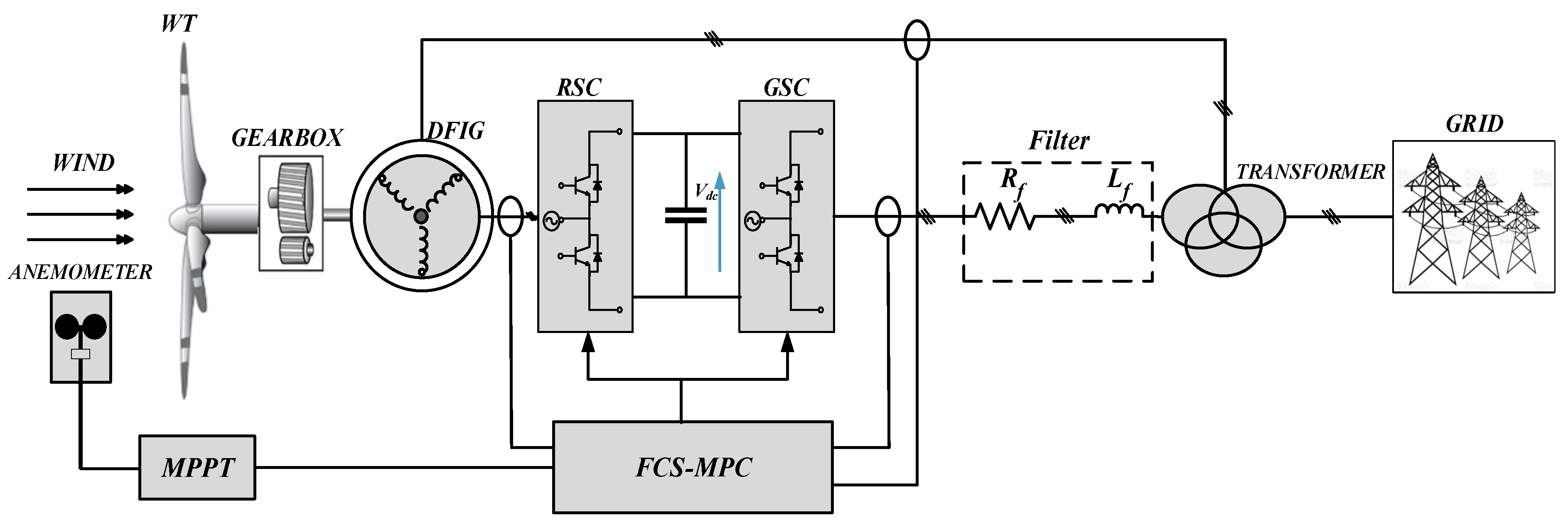
2. Modeling of The Wind Turbine System with DFIG

The wind turbine conversion chain on which this paper is based is a wind turbine, a gearbox, a doubly fed asynchronous generator (DFIG), a DC bus and two static power converters. The wind turbine drives the DFIG at a variable rotation speed through a speed multiplier. The stator of the DFIG is directly connected to the electrical grid. In contrast, the rotor is connected to the grid via two static converters (Inverter + Rectifier) cascaded through a DC bus.

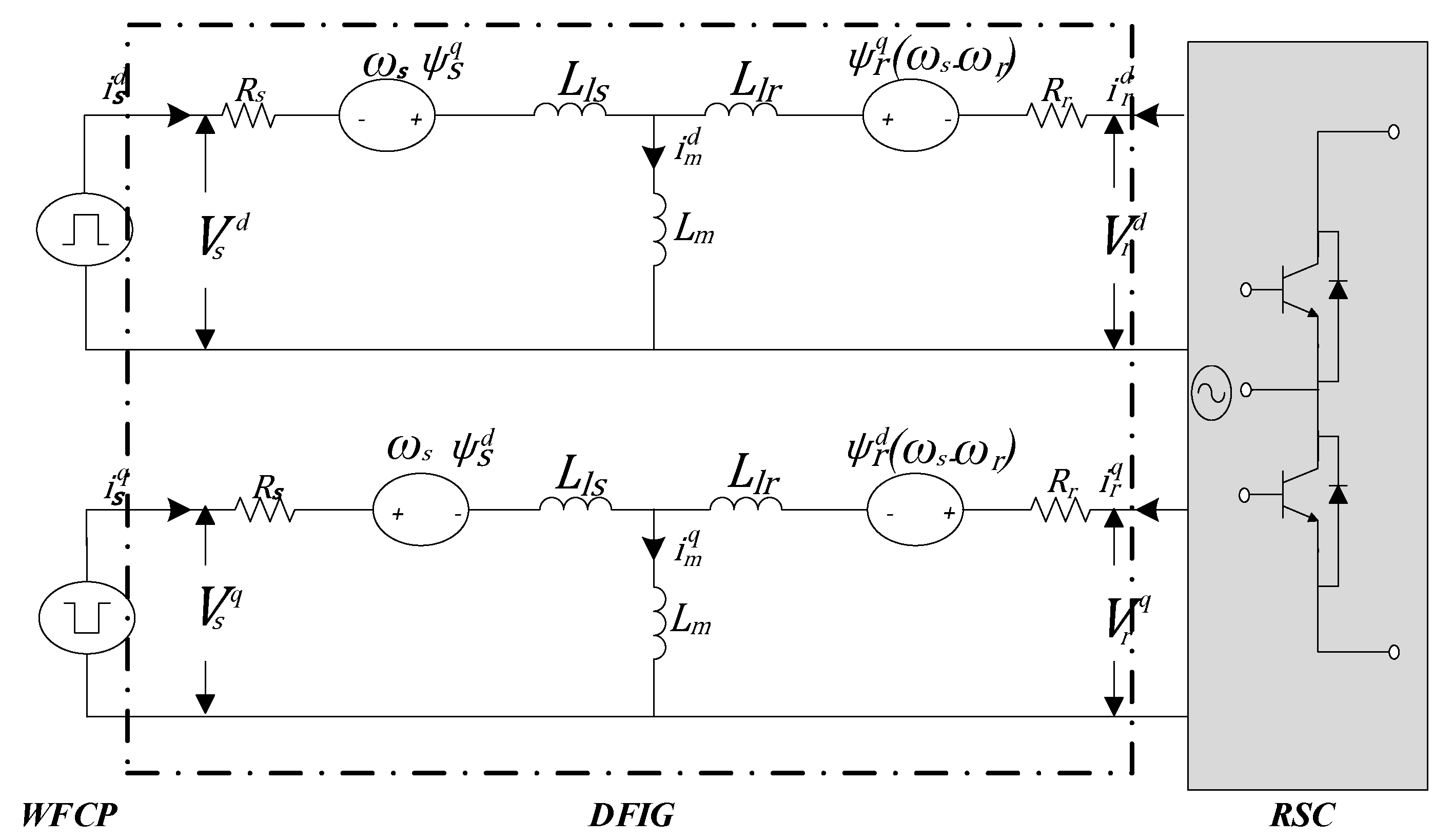
2.1. Modeling of the DFIG

The model of the DFIG machine can be schematized as in Figure 2 [14].

The voltage equations of the stator and rotor of the DFIG in the rotating reference frame dq (Park transformation) are given by:

$$\{\begin{array}{c}{V}_s^J\left(t\right)=R_s{i}_s^J\left(t\right)+\frac{d}{dt}{\psi }_s^J\left(t\right)+j{\omega }_s{\psi }_s^J\left(t\right) \\ V_r^J\left(t\right)=R_r{i}_r^J\left(t\right)+\frac{d}{dt}{\psi }_r^J\left(t\right)+j({\omega }_s-{\omega }_r){\psi }_r^J\left(t\right) \end{array}$$

(1)

where $V_s^J\left(t\right)=\left(\begin{array}{c}{V}_s^d\\ V_s^q\end{array}\right)$, $V_r^J\left(t\right)=\left(\begin{array}{c}{V}_r^d\\ V_r^q\end{array}\right)$, $i_s^J\left(t\right)=\left(\begin{array}{c}{i}_s^d\\ i_s^q\end{array}\right)$, $i_r^J\left(t\right)=\left(\begin{array}{c}{i}_r^d\\ i_r^q\end{array}\right)$, ${\psi }_s^J\left(t\right)=\left(\begin{array}{c}{\psi }_s^d\\ {\psi }_s^q\end{array}\right)$, ${\psi }_r^J\left(t\right)=\left(\begin{array}{c}{\psi }_r^d\\ {\psi }_r^q\end{array}\right)$, j = $\left(\begin{array}{cc}0& -1\\ 1& 0\end{array}\right)$, ${\omega }_s$, and ${\omega }_r$ are the stator and rotor voltages, currents, and fluxes, $L_s,L_r$, and $L_m$ are the inductances of the machine, $R_r,R_s$ are the rotor and the stator resistances, and $P_p$ is the number of pair poles.

The flux linkages are expressed as:

$$\{\begin{array}{c}{\psi }_s^J\left(t\right)=L_s{i}_s^J\left(t\right)+L_m{i}_r^J\left(t\right)\\ {\psi }_r^J\left(t\right)=L_s{i}_r^J\left(t\right)+L_m{i}_s^J\left(t\right)\end{array}$$

(2)

The electromagnetic torque is:

$$T_e\left(t\right)=\frac{3}{2}{P}_p\left({\psi }_s^d\left(t\right)i_s^q\left(t\right)-{\psi }_s^q\left(t\right)i_s^d\left(t\right)\right)$$

(3)

2.2. Converter and DC-Bus

The variable V_out of the RSC and GSC can be calculated by [15,16]:

$$\{\begin{array}{c}{V}_r^K\left(t\right)=\frac{1}{3}{V}_{dc}\left(t\right)T^K{S}_r^k\left(t\right)\\ V_f^K\left(t\right)=\frac{1}{3}{V}_{dc}\left(t\right)T^K{S}_f^k\left(t\right)\end{array}$$

(4)

where $V_r^K\left(t\right)=\left(\begin{array}{c}{V}_r^a\\ V_r^b\\ V_r^c\end{array}\right),V_f^K\left(t\right)=\left(\begin{array}{c}{V}_f^a\\ V_f^b\\ V_f^c\end{array}\right),S_r^K\left(t\right)=\left(\begin{array}{c}{S}_r^a\\ S_r^b\\ S_r^c\end{array}\right)$, and $S_f^K\left(t\right)=\left(\begin{array}{c}{S}_f^a\\ S_f^b\\ S_f^c\end{array}\right)$ are the switching state vectors of the RSC and GSC and ${\mathrm{T}}^{\mathrm{K}}$ is the transformation matrix:

$$T^K\left(t\right)=\left(\begin{array}{ccc}2& -1& -1\\ -1& 2& -1\\ -1& -1& 2\end{array}\right)$$

(5)

Considering the converter’s eight switching states (Figure 3), we consequently obtain eight voltage vectors represented in the figure. The dynamics of the DC link are given in Figure 3 [16,17].

3. Continuous-Time Dynamic Models of DFIG

The dynamic continuous-time (CT) model of the currents is given as follows [18]:

$$\frac{d}{dt}\left(\begin{array}{c}{i}_s^d\\ i_s^q\\ {\psi }_r^d\\ {\psi }_d^q\end{array}\right)=\left(\begin{array}{cccc}-\frac{1}{{\tau }_{\sigma }}& {\omega }_s& \frac{k_r}{L_s{\sigma \tau }_r}& \frac{k_r{\omega }_r}{\sigma L_s}\\ -{\omega }_s& -\frac{1}{{\tau }_{\sigma }}& -\frac{k_r{\omega }_r}{\sigma L_s}& \frac{k_r}{L_s{\sigma \tau }_r}\\ \frac{L_m}{{\tau }_r}& 0& -\frac{1}{{\tau }_{\sigma }}& {(\omega }_s-{\omega }_r)\\ 0& \frac{L_m}{{\tau }_r}& -{(\omega }_s-{\omega }_r)& -\frac{1}{{\tau }_{\sigma }}\end{array}\right)\left(\begin{array}{c}{i}_s^d\\ i_s^q\\ {\psi }_r^d\\ {\psi }_d^q\end{array}\right)+\left(\begin{array}{cccc}\frac{1}{L_s\sigma }& 0& -\frac{k_r}{L_s\sigma }& 0\\ 0& -\frac{1}{{\tau }_{\sigma }}& -\frac{k_r{\omega }_r}{\sigma L_s}& \frac{k_r}{L_s{\sigma \tau }_r}\\ 0& 0& 1& 0\\ 0& 0& 0& 1\end{array}\right)\left(\begin{array}{c}{V}_s^d\\ V_s^q\\ V_r^d\\ V_d^q\end{array}\right)$$

(6)

The output model CT, which relates the rotor currents with the state variables, is given by:

$$\left(\begin{array}{c}{i}_r^d\\ i_r^q\end{array}\right)=\left(\begin{array}{cccc}-\frac{L_m}{L_r}& 0& \frac{1}{L_r}& 0\\ 0& -\frac{L_m}{L_r}& 0& \frac{1}{L_r}\end{array}\right)\left(\begin{array}{c}{i}_s^d\\ i_s^q\\ {\psi }_r^d\\ {\psi }_d^q\end{array}\right)$$

(7)

The direct dynamic model of the rotor currents can be obtained as follows [19]:

$$\begin{gathered} \frac{d}{dt}\left(\begin{array}{c}{i}_s^d\\ i_s^q\\ i_r^d\\ i_d^q\end{array}\right)=k_{\sigma }\left(\begin{array}{cccc}-R_s{L}_r& {\omega }_r{L}_m^2+k_{\omega }& R_r{L}_m& {\omega }_r{L}_m{L}_r\\ -{\omega }_r{L}_m^2-k_{\omega }& -R_s{L}_r& -{\omega }_r{L}_m{L}_r& R_r{L}_m\\ R_s{L}_m& {-\omega }_r{L}_s{L}_m& -R_r{L}_s& -{\omega }_r{L}_s{L}_r+k_{\omega }\\ {\omega }_r{L}_s{L}_m& R_s{L}_m& {\omega }_r{L}_s{L}_r-k_{\omega }& -R_r{L}_s\end{array}\right)\left(\begin{array}{c}{i}_s^d\\ i_s^q\\ i_r^d\\ i_d^q\end{array}\right) \\ +k_{\sigma }\left(\begin{array}{cccc}{L}_r& 0& -L_m& 0\\ 0& L_r& 0& -L_m\\ -L_m& 0& 1& 0\\ 0& -L_m& 0& L_s\end{array}\right)\left(\begin{array}{c}{V}_s^d\\ V_s^q\\ V_r^d\\ V_d^q\end{array}\right) \end{gathered}$$

(8)

with:

$$k_{\sigma }=\frac{1}{{\sigma L}_s{L}_r},k_{\omega }={{\omega }_s\sigma L}_s{L}_r,$$

(9)

4. FCS-MPC Strategy

The fundamental principle of the FCS-MPC technique [14] permits us to consider future behavior by using the system’s numerical model to predict the output’s future behavior on a finite horizon. The main idea presented in this paper is to predict all the possible variables of the system on a sampling period; this prediction has been performed on a limited number thanks to the finite number of switching states S_i (i = 1, …, n) to solve the optimization problem, then the calculation of the reference voltage that minimizes the cost function has been performed at each sampling period in order to apply it to the next time (K + 1) [20,21].

The novelty in this paper is to propose a cost function which can allows both to give satisfactory results and at the same time does not impact the calculation time. The primary and secondary cost functions are represented in the generic form which can be realized as follows:

$$g\left(k\right)=\left|\right|x^{*}\left(k+1\right)-x^p\left(k+1\right)\left|\right|$$

(10)

where $x^{*}$ is the extrapolated reference command and $x^p$ is the predicted value of the command variable; both correspond to the sampling time (k + 1). The expression 1 is a distance measure between $x^{*}$ and $x^p$ can be written as an absolute value Equation (2), squared value Equation (3), or exponential Equation (4). However, the last approach requires a larger number of calculations:

$$g\left(k\right)=\left|x^{*}-x^p\right|$$

(11)

$$g\left(k\right)={\left(x^{*}-x^p\right)}^2$$

(12)

$$g\left(k\right)=exp\left|x^{*}-x^p\right|$$

(13)

In this article, the authors have implemented the cost function in the form below, which allows to give satisfactory results and at the same time does not impact the calculation time:

$$g_r=\left|{\widehat{i}}_{r,ref}^d\left(k+1\right)-i_r^d\left(k+1\right)\right|+\left|+{\widehat{i}}_{r,ref}^d\left(k+1\right)-i_r^q\left(k+1\right)\right|$$

(14)

Therefore, it is generally necessary to use sampled data models from the corresponding CT models to obtain the optimal FCS-MPC control. The continuous representation of a system is [21,22]:

$$\{\begin{array}{c}\frac{d}{dt}x\left(t\right)=A\dot{x}\left(t\right)+Bu\left(t\right)\hfill \\ y\left(t\right)=Cx\left(t\right)\hfill \end{array}$$

(15)

where A and B represent the converter’s CT settings (filter inductance, DC-link capacitance, etc.). In continuous time, u(t) is the input vector (DC voltage, grid voltage, etc.), and x(t) is the state vector to be managed (voltage, current, power, torque, flux, etc.). The discrete model of the system (5) by the Euler method is given by the following relation [22]:

$${\left\{\frac{dx\left(t\right)}{dt}\right\}}_{t=k}=\frac{x\left(k+1\right)-x\left(k\right)}{T_s}$$

(16)

Therefore:

x(k + 1) = Πx (k) + Φu (k)

(17)

$$\Pi \approx I+A{T}_s, \Phi \approx B{T}_s$$

(18)

where I is a matrix with the same dimension as matrix A. However, the calculation of Φ and Π involves an exponential matrix, as demonstrated below:

$$\Pi e^{A{T}_s},\Phi ={{\displaystyle \int }}_0^{T_s}{e}^{A\tau }d\tau =A^{-1} (\Pi -I)B$$

(19)

5. Model Predictive Control

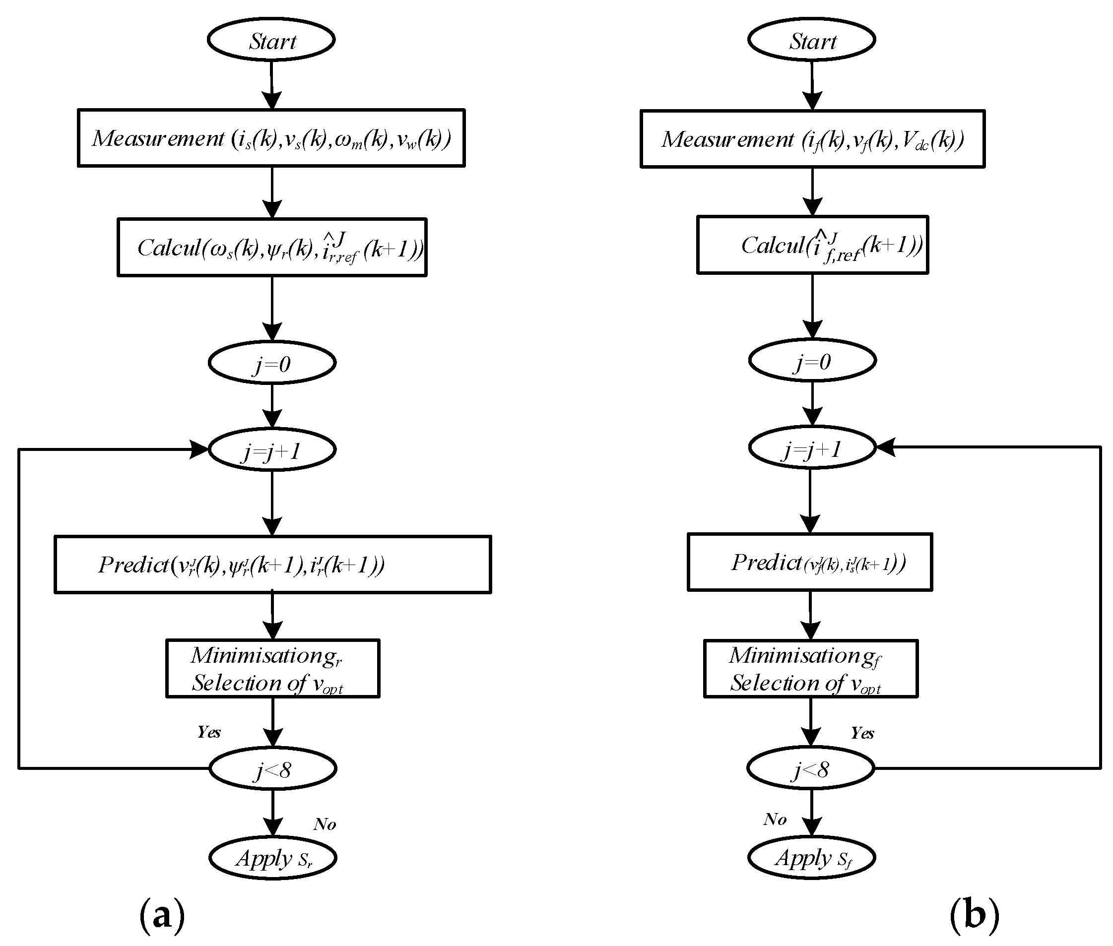
5.1. MPC Control for RSC

The rotor voltage ${\mathrm{V}}_{\mathrm{r}}^{\mathrm{J}}$ of the DFIG (t) can be expressed as:

$$\left(\begin{array}{c}{V}_r^d\left(t\right)\\ V_r^q\left(t\right)\end{array}\right)=R_r\left(\begin{array}{c}{i}_r^d\left(t\right)\\ i_r^q\left(t\right)\end{array}\right)+L_r\frac{d}{dt}\left(\begin{array}{c}{i}_r^d\left(t\right)\\ i_r^q\left(t\right)\end{array}\right)+L_m\frac{d}{dt}\left(\begin{array}{c}{i}_s^d\left(t\right)\\ i_s^q\left(t\right)\end{array}\right)+ ({\omega }_s-{\omega }_r)L_{r}j\left(\begin{array}{c}{i}_r^d\left(t\right)\\ i_r^q\left(t\right)\end{array}\right)+({\omega }_s-{\omega }_r)L_{m}j\left(\begin{array}{c}{i}_s^d\left(t\right)\\ i_s^q\left(t\right)\end{array}\right)$$

(20)

or:

$$\left(\begin{array}{c}{i}_s^d\left(t\right)\\ i_s^q\left(t\right)\end{array}\right)=\frac{1}{L_s}\left(\begin{array}{c}{\psi }_s^d\left(t\right)\\ {\psi }_s^q\left(t\right)\end{array}\right)-\frac{L_m}{L_s}\left(\begin{array}{c}{i}_r^d\left(t\right)\\ i_r^q\left(t\right)\end{array}\right)$$

(21)

Equation (20) can be rewritten as:

$$\left(\begin{array}{c}{V}_r^d\left(t\right)\\ V_r^q\left(t\right)\end{array}\right)=R_r\left(\begin{array}{c}{i}_r^d\left(t\right)\\ i_r^q\left(t\right)\end{array}\right)+\gamma L_r\frac{d}{dt}\left(\begin{array}{c}{i}_r^d\left(t\right)\\ i_r^q\left(t\right)\end{array}\right)+\frac{L_m}{L_s}\frac{d}{dt}\left(\begin{array}{c}{\psi }_s^d\left(t\right)\\ {\psi }_s^q\left(t\right)\end{array}\right)+ {\omega }_{sl}{L}_r\gamma j\left(\begin{array}{c}{i}_r^d\left(t\right)\\ i_r^q\left(t\right)\end{array}\right)+{\omega }_{sl}\frac{L_m}{L_s}j\left(\begin{array}{c}{\psi }_s^d\left(t\right)\\ {\psi }_s^q\left(t\right)\end{array}\right)$$

(22)

where ${\omega }_{sl}=\left( {\omega }_s-{\omega }_r\right)$ is the generator angular slip frequency and $\gamma =1-\frac{L_m^2}{L_s{L}_r}$. By replacing ${\psi }_s^J$ and $\frac{d{\psi }_s^J}{dt}$ by their values, we find:

$$\left(\begin{array}{c}{V}_r^d\left(t\right)\\ V_r^q\left(t\right)\end{array}\right)=R_r\left(\begin{array}{c}{i}_r^d\left(t\right)\\ i_r^q\left(t\right)\end{array}\right)+\gamma L_r\frac{d}{dt}\left(\begin{array}{c}{i}_r^d\left(t\right)\\ i_r^q\left(t\right)\end{array}\right)+\left( {\omega }_{sl}\left(t\right)L_r-{\omega }_s\left(t\right)\frac{L_m^2}{L_s}\right)j\left(\begin{array}{c}{i}_r^d\left(t\right)\\ i_r^q\left(t\right)\end{array}\right)-\left(R_{s }\frac{L_m}{L_s}+{\omega }_r\left(t\right)L_m\right)j\left(\begin{array}{c}{i}_s^d\left(t\right)\\ i_s^q\left(t\right)\end{array}\right)+\frac{L_m}{L_s}\left(\begin{array}{c}{V}_s^d\left(t\right)\\ V_s^q\left(t\right)\end{array}\right)$$

(23)

Then:

$$\begin{gathered} \frac{d}{dt}\left(\begin{array}{c}{i}_r^d\left(t\right)\\ i_r^q\left(t\right)\end{array}\right)=\frac{1}{\gamma L_s{L}_r}\left[-R_s{L}_r\left(\begin{array}{c}{i}_r^d\left(t\right)\\ i_r^q\left(t\right)\end{array}\right)+{(\omega }_{sl}{\left(k\right)L}_r{L}_s-{\omega }_s{L}_m^2)j\left(\begin{array}{c}{i}_r^d\left(t\right)\\ i_r^q\left(t\right)\end{array}\right)+R_s{L}_m\left(\begin{array}{c}{i}_s^d\left(t\right)\\ i_s^q\left(t\right)\end{array}\right)+{\omega }_r{L}_m{L}_{s}j\left(\begin{array}{c}{i}_s^d\left(t\right)\\ i_s^q\left(t\right)\end{array}\right)+ \\ {L}_s\left(\begin{array}{c}{V}_s^d\left(t\right)\\ V_s^q\left(t\right)\end{array}\right)-L_m\left(\begin{array}{c}{V}_r^d\left(t\right)\\ V_r^q\left(t\right)\end{array}\right)\right] \end{gathered}$$

(24)

Therefore, the discrete model of DFIG can be expressed as follows:

$$\begin{gathered} \left(\begin{array}{c}{i}_r^d(k+1)\\ i_r^q(k+1)\end{array}\right)=\left(\begin{array}{c}{i}_r^d\left(k\right)\\ i_r^q\left(k\right)\end{array}\right)+\frac{T_s}{\gamma L_r{L}_s}\left[-R_r{L}_s\left(\begin{array}{c}{i}_r^d\left(k\right)\\ i_r^q\left(k\right)\end{array}\right)+\left({\omega }_{sl}{\left(k\right)L}_r{L}_s-{\omega }_s{L}_m^2\right)j\left(\begin{array}{c}{i}_r^d\left(k\right)\\ i_r^q\left(k\right)\end{array}\right)+R_s{L}_m\left(\begin{array}{c}{i}_s^d\left(K\right)\\ i_s^q\left(K\right)\end{array}\right)+ \\ {\omega }_r(k)L_m{L}_{s}j\left(\begin{array}{c}{i}_s^d\left(k\right)\\ i_s^q\left(k\right)\end{array}\right){+L}_s\left(\begin{array}{c}{V}_r^d\left(k\right)\\ V_r^q\left(k\right)\end{array}\right)-L_m\left(\begin{array}{c}{V}_s^d\left(k\right)\\ V_s^q\left(k\right)\end{array}\right)\right] \end{gathered}$$

(25)

The cost function of the RSC is defined by:

$$g_r=\left|{\widehat{i}}_{r,ref}^d\left(k+1\right)-i_r^d\left(k+1\right)\right|+\left|+{\widehat{i}}_{r,ref}^q\left(k+1\right)-i_r^q\left(k+1\right)\right|$$

(26)

In the MPC method, the current is estimated seven times using the seven voltage vectors of the converter. Then, each of the seven anticipated currents is evaluated concerning the cost function to obtain the voltage vector that minimizes the cost function. The current and past values of the reference current are used to calculate the expected currents using Lagrange extrapolation as follows:

$${\widehat{i}}_{r,ref}^J\left(k+1\right)=2i_{r,ref}^J\left(k\right)-i_{r,ref}^J\left(k-1\right)$$

(27)

Then:

$$i_{r,ref}^d\left(k\right)=\frac{2{\omega }_s\left(k\right)L_s}{3P_p{L}_m{V}_s^d\left(k\right)}{T}_{e,ref}\left(k\right)\mathrm{and}{i}_{r,ref}^q\left(k\right)=\frac{2L_s}{3L_m{V}_s^d\left(k\right)}{Q}_{s,ref}\left(k\right)-\frac{V_s^d\left(k\right)}{{\omega }_s\left(k\right)L_s}$$

(28)

5.2. MPC Control for GSC

The discrete model of the current of the grid can be expressed as follows:

$$\left(\begin{array}{c}{i}_f^d\left(k+1\right)\\ i_f^d\left(k+1\right)\end{array}\right)=\left(1-\frac{T_s{R}_f}{L_f}\right)\left(\begin{array}{c}{i}_f^d\left(k\right)\\ i_f^d\left(k\right)\end{array}\right)+\left(\begin{array}{cc}0& {\omega }_e{T}_s\\ -{\omega }_e{T}_s& 0\end{array}\right)\left(\begin{array}{c}{i}_f^d\left(k\right)\\ i_f^q\left(k\right)\end{array}\right)+\frac{T_s}{L_f}\left(\begin{array}{c}{V}_s^d\left(k\right)\\ V_s^q\left(k\right)\end{array}\right)-\frac{T_s}{L_f }\left(\begin{array}{c}{V}_f^d\left(k\right)\\ V_f^q\left(k\right)\end{array}\right)$$

(29)

The cost function is calculated by:

$$g_r=\left|{\widehat{i}}_{r,ref}^d\left(k+1\right)-i_f^d\left(k+1\right)\right|+\left|+{\widehat{i}}_{r,ref}^q\left(k+1\right)-i_f^q\left(k+1\right)\right|$$

(30)

Similar to the RSC case, the voltage vector that minimizes the cost function will be applied at the future time (k + 1). The reference current $i_{f,ref}^j(k+1)$ is calculated by Lagrange extrapolation:

$$i_{f,ref}^q\left(k\right)=-\frac{2Q_{f,ref}\left(k\right)}{3V_s^d\left(k\right)}$$

(31)

The proposed predictive control strategy is shown in Figure 4. The overall system is realized on the MATLAB/Simulink platform to validate the proposed theoretical approach [23,24].

The flowcharts of the dq-frame MPC algorithms for RSC (a) and GSC (b) are presented in Figure 5. The numerical design of both algorithms is similar, consisting of eight steps. The first block presents the measured parameters, and the extrapolation of the currents in dq is given in the second block. The PCC algorithm is started in block 3, the predicted currents and voltages are given in block 5, and the minimization of the cost function and selection of the optimal voltage vector are given in block 6. After completing an iterative loop for eight values of counter, the switch signals corresponding to $g_{op}$ are applied to the converter.

6. Simulation Results

In order to evaluate the effectiveness and robustness of the control proposed in this work, the system has been subjected to two validation tests in the MATLAB/Simulink program. First, a stepped wind profile is applied to the system. The wind here is considered constant. Figure 6 represents the results obtained when applying the MPC to the system (

Table 1. The DFIG and wind turbine parameters.

PMSG Parameters		Wind Turbine Parameters
Power Generator Stator Resistance Rotor Resistance Stator inductance Rotor inductance DC Link Voltage	Ps = 1.5 Kw Rs = 4.85 Ω Rr = 3.805 Ω Ls = 274 mH Lr = 258 mH Vdc = 600 V	Radius of the turbine blade Density of air Tip speed Ratio Optimal Power Coefficient	R = 20 m ρ = 1.225 kg/m3 λopt = 8 Cp = 0.45

).

7. Discussion

First, Figure 6a shows the wind profile used. The stepwise wind variations are as follows: at t = 3 s, t = 5 s, and t = 9 s. From these results, we note that (Figure 6):

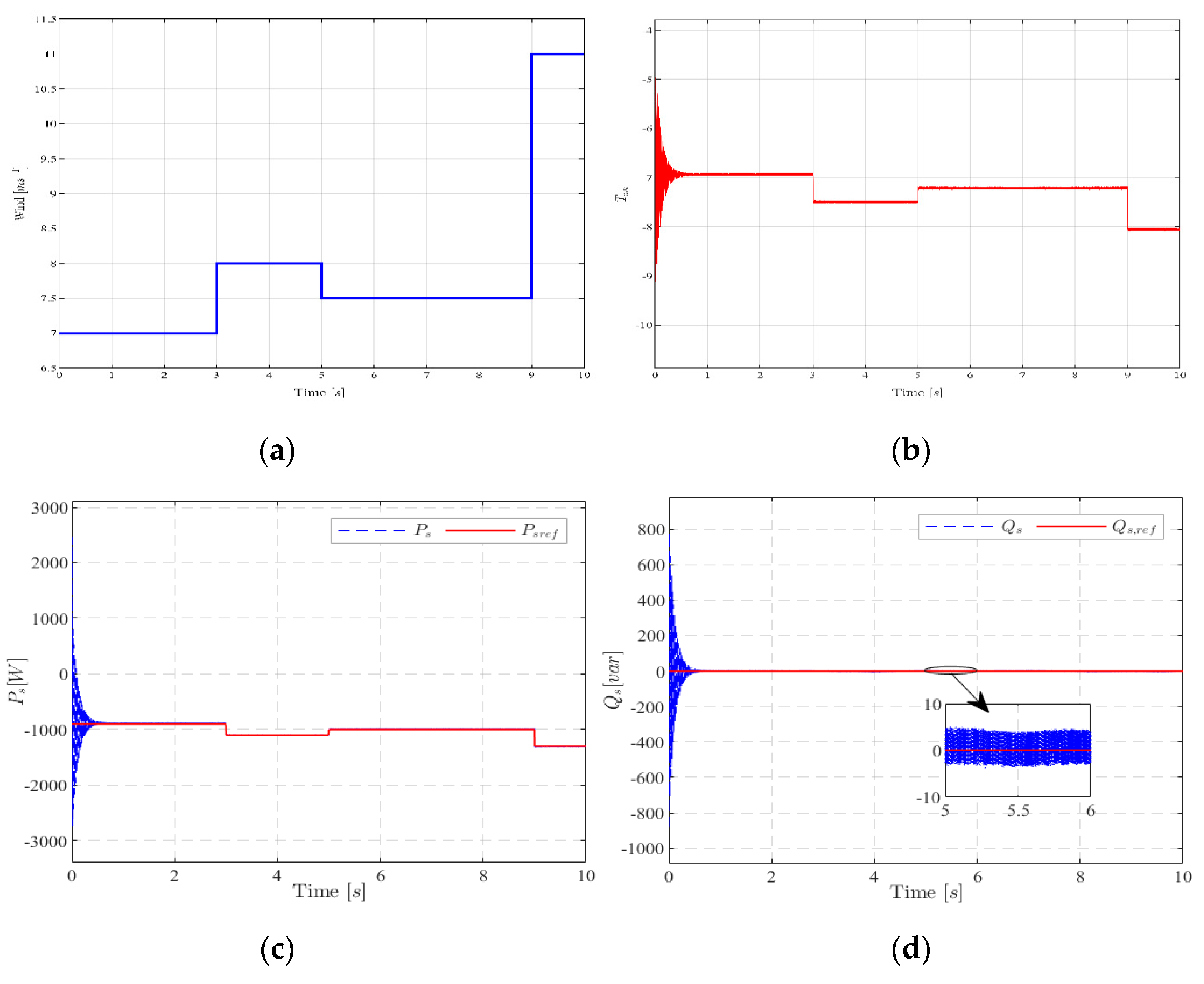
• The decoupling between the active and reactive powers of the stator is assured;
• The electromagnetic torque (Figure 6b) depends directly on the active power—its similar shape reflects this to that of the active power;
• The negative value of the stator power $P_s$ (Figure 6c) explains the operation of the machine in generator model;
• The reactive power is equal to zero (Figure 6d), indicating the uniqueness of the power factor;
• The quadrature rotor current $I_{qr}$ varies linearly with $P_s$ with a negative coefficient described in the Equation (26), which is illustrated in Figure 6e;
• The direct rotor current $I_{rd}$ depends on the stator reactive power $Q_s$—according to Figure 6f, the trend of the direct current has a constant value of about 5 A, due to the ratio ${\psi }_s$/$L_m$;
• The evolution of the rotor and stator currents (Figure 6g,h) in three-phase abc keeps a sinusoidal form, which implies a frequency of a value 50 Hz, which indicates a better quality of the energy injected into the network;
• The DC bus (Figure 6i) follows its reference value with a small error and an overrun of 8.3%.

In order to analyze the behavior of the MADA in a dynamic regime, a random wind profile is applied. Its form is illustrated in Figure 7.

Secondly, a fixed random wind profile (Figure 7a) is applied to the system to illustrate the effectiveness of the proposed control with wind variation.

From these results, we note that (Figure 7):

• The decoupling between the active and reactive powers of the stator is assured;
• The electromagnetic torque (Figure 7b) depends directly on the active power—its similar shape reflects this to that of the active power;
• The negative value of the stator power $P_s$ (Figure 7c) explains the operation of the machine in generator mode;
• The reactive power is zero (Figure 7d), indicating the uniqueness of the power factor;
• The quadrature rotor current $I_{qr}$ varies linearly with $P_s$ with a negative coefficient described in Equation (26), which is illustrated in (Figure 7e);
• The direct rotor current $I_{rd}$ depends on the stator reactive power $Q_s$—according to Figure 7f, the trend of the direct current has a constant value of about 5 A, due to the ratio ${\psi }_s$/$L_m$;
• The evolution of the rotor and stator currents (Figure 7g,h) in three-phase abc keeps a sinusoidal form, which implies a frequency of a value 50 Hz, which implies a better quality of the energy injected into the network;
• The DC bus (Figure 7i) follows its reference value with a small error.

A comparison between the command proposed in this work with other controls existing in the literature is summarized in

Table 2. Performance’s comparison.

Publication Paper	Technical Methods	Response Time(s)	Error (%)	THD (%)
[25]	Fuzzy SMC	0.32	-	-
[26]	PI	0.030	1.25	-
	RST	0.028	0.06	-
[27]	SMC-based Backstepping	0.05	-	2.98
[28]	DTC	0.12	-	18.8
	FSC	0.16	-	8.26
	MPDC	0.15	-	8.17
[29]	FCSMPC	0.15	-	6.12
[30]	FCSMPC	0.12	-	4.29
Proposed technique	FCS-MPC	0.11	0.11	0.49

.

A comparison of the results between the proposed control and other studies is presented in Table 2. Although the error of the proposed technique is minimized compared to [26], the most significant advantage of this control is the minimization of THD compared to [27,28,29,30], which did not exceed 0.49%, indicating excellent power quality and response time minimization.

8. Conclusions

This study proposes an upgraded model predictive control strategy to improve the performance and efficiency of the DFIG-based Wind Energy Conversion System. While the main objective is error minimization, this study proposed an FCS-MPC based on a novel cost function. An appropriate cost function has been proposed that allows to both give satisfactory results and not impact the computation time.

To accomplish these goals, the system was first introduced, then the FSC technique was explained, and ultimately, this approach was used to control the rotor and array. A random wind profile was employed to assess the system performance using a unit power factor. The simulation results are displayed using a 1.5 kW dual-fed induction generator in a MATLAB/Simulink system.

The simulation results show that the proposed control strategy can have very good performance tracking by providing an error of 0.11% and a response time of 0.11%.

References

- El Alami, H.; Bossoufi, B.; Motahhir, S.; Alkhammash, E.H.; Masud, M.; Karim, M.; Taoussi, M.; Bouderbala, M.; Lamnadi, M.; El Mahfoud, M. FPGA in the Loop Implementation for Observer Sliding Mode Control of DFIG-Generators for Wind Turbines. Electronics 2021, 11, 116. [Google Scholar] [CrossRef]
- Bossoufi, B.; Karim, M.; Taoussi, M.; Aroussi, H.A.; Bouderbala, M.; Deblecker, O.; Motahhir, S.; Nayyar, A.; Alzain, M.A. Rooted tree optimization for the backstepping power control of a doubly fed induction generator wind turbine: dSPACE implementation. IEEE Access 2021, 9, 26512–26522. [Google Scholar] [CrossRef]
- El Mahfoud, M.; Bossoufi, B.; El Ouanjli, N.; Mahfoud, S.; Yessef, M.; Taoussi, M. Speed Sensorless Direct Torque Control of Doubly Fed Induction Motor Using Model Reference Adaptive System. In Proceedings of the International Conference on Digital Technologies and Applications, Fez, Morocco, 29–30 January 2021; pp. 1821–1830. [Google Scholar]
- Ekanayake, J.; Holdsworth, L.; Jenkins, N. Control of DFIG wind turbines. Power Eng. 2003, 17, 28–32. [Google Scholar] [CrossRef]
- Kayikci, M.; Milanovic, J.V. Reactive power control strategies for DFIG-based plants. IEEE Trans. Energy Convers. 2007, 22, 389–396. [Google Scholar]
- El Alami, H.; Bossoufi, B.; El Mahfoud, M.; Btissam, M.; Yessef, M.; Bekkour, E.H.; Salime, H. Improved Performance of Wind Turbines Based on Doubly Fed Generator Using the IFOC-SVM Control. In Proceedings of the International Conference on Digital Technologies and Applications, Fez, Morocco, 28–30 January 2022; pp. 812–822. [Google Scholar]
- Hu, J.; He, Y.; Xu, L.; Williams, B.W. Improved control of DFIG systems during network unbalance using PI–R current regulators. IEEE Trans. Ind. Electron. 2008, 56, 439–451. [Google Scholar] [CrossRef]
- Tavakoli, S.M.; Pourmina, M.A.; Zolghadri, M.R. Comparison between different DPC methods applied to DFIG wind turbines. Int. J. Renew. Energy Res. 2013, 3, 446–452. [Google Scholar]
- Emeksiz, C.; Demirci, B. The determination of offshore wind energy potential of Turkey by using novelty hybrid site selection method. Sustain. Energy Technol. Assess. 2019, 36, 100562. [Google Scholar] [CrossRef]
- Benamor, A.; Benchouia, M.T.; Srairi, K.; Benbouzid, M.E.H. A new rooted tree optimization algorithm for indirect power control of wind turbine based on a doubly-fed induction generator. ISA Trans. 2019, 88, 296–306. [Google Scholar] [CrossRef]
- Boubzizi, S.; Abid, H.; El Hajjaji, A.; Chaabane, M. Comparative study of three types of controllers for DFIG in wind energy conversion system. Prot. Control Mod. Power Syst. 2018, 3, 1–12. [Google Scholar] [CrossRef]
- Abad, G.; López, J.; Rodríguez, M.A.; Marroyo, L.; Iwanski, G. Doubly Fed Induction Machine: Modeling and Control for Wind Energy Generation; John Wiley and Sons: Hoboken, NJ, USA, 2011. [Google Scholar]
- Majout, B.; El Alami, H.; Salime, H.; Zine Laabidine, N.; El Mourabit, Y.; Motahhir, S.; Bouderbala, M.; Karim, M.; Bossoufi, B. A Review on Popular Control Applications in Wind Energy Conversion System Based on Permanent Magnet Generator PMSG. Energies 2022, 15, 6238. [Google Scholar] [CrossRef]
- Ayyarao, T.S.L.V. Modified vector controlled DFIG wind energy system based on barrier function adaptive sliding mode control. Prot. Control Mod. Power Syst. 2019, 4, 4. [Google Scholar] [CrossRef]
- Allam, M.; Dehiba, B.; Abid, M.; Djeriri, Y.; Adjoudj, R. Etude comparative entre la commande vectorielle directe et indirecte de la Machine Asynchrone à Double Alimentation (MADA) dédiée à une application éolienne. J. Adv. Res. Sci. Technol. 2014, 1, 88–100. [Google Scholar]
- Abdelrahem, M.; Hackl, C.; Kennel, R. Encoderless model predictive control of doubly-fed induction generators in variable-speed wind turbine systems. In Proceedings of the Science of Making Torque from Wind (TORQUE 2016) Conference, Munich, Germany, 5–7 October 2016. [Google Scholar]
- Mohammed, E.M.; Badre, B.; Najib, E.O.; Abdelilah, H.; Houda, E.A.; Btissam, M.; Said, M. Predictive Torque and Direct Torque Controls for Doubly Fed Induction Motor: A Comparative Study. In Proceedings of the International Conference on Digital Technologies and Applications, Fez, Morocco, 28–30 January 2022; pp. 825–835. [Google Scholar]
- Holtz, J. The representation of AC machine dynamics by complex signal flow graphs. IEEE Trans. Ind. Electron. 1995, 42, 263–271. [Google Scholar] [CrossRef]
- Holtz, J. Sensorless control of induction motor drives. Proc. IEEE 2002, 90, 1359–1394. [Google Scholar] [CrossRef]
- Zhi, D.; Xu, L.; Williams, B.W. Model-based predictive direct power control of doubly fed induction generators. IEEE Trans. Power Electron. 2010, 25, 341–351. [Google Scholar]
- Rodriguez, J.; Cortes, P. Predictive Control of Power Converters and Electrical Drives, 1st ed.; Wiley-IEEE Press: New York, NY, USA, 2012. [Google Scholar]
- Wang, F.; Li, S.; Mei, X.; Xie, W.; Rodriguez, J.; Kennel, R. Model-based predictive direct control strategies for electrical drives: An experimental evaluation of PTC and PCC methods. IEEE Trans. Ind. Inform. 2015, 11, 671–681. [Google Scholar] [CrossRef]
- Akter, P.; Mekhilef, S.; Tan, N.M.L.; Akagi, H. Modified model predictive control of a bidirectional AC-DC converter based on lyapunov function for energy storage systems. IEEE Trans. Ind. Electron. 2016, 63, 704–715. [Google Scholar] [CrossRef]
- Wu, B.; Lang, Y.; Zargari, N.; Kouro, S. Power Conversion and Control of Wind Energy Systems; Wiley-IEEE Press: New York, NY, USA, 2011. [Google Scholar]
- Echiheb, F.; Ihedrane, Y.; Bossoufi, B.; Bouderbala, M.; Motahhir, S.; Masud, M.; Aljahdali, S.; El Ghamrasni, M. Robust Sliding-Backstepping mode Control of a wind system based on the DFIG Generator. Sci. Rep. 2022, 12, 11782. [Google Scholar] [CrossRef]
- Djeriri, Y.; Meroufel, A.; Massoum, A.; Boudjema, Z. A comparative study between field oriented control strategy and direct power control strategy for DFIG. J. Electr. Eng. 2014, 14, 9. [Google Scholar]
- Hansen, A.D.; Michalke, G. Fault ride-through capability of DFIG wind turbines. Renew. Energy 2007, 32, 1594–1610. [Google Scholar] [CrossRef]
- Yang, X.; Liu, G.; Le, V.D.; Le, C.Q. A novel model-predictive direct control for induction motor drives. IEEJ Trans. Electr. Electron. Eng. 2019, 14, 1691–1702. [Google Scholar] [CrossRef]
- Kou, P.; Liang, D.; Li, J.; Gao, L.; Ze, Q. Finite-Control-Set Model Predictive Control for DFIG Wind Turbines. IEEE Trans. Autom. Sci. Eng. 2018, 15, 1004–1013. [Google Scholar] [CrossRef]
- Bouderbala, M.; Bossoufi, B.; Alami Aroussi, H.; Taoussi, M.; Lagrioui, A. Novel deadbeat predictive control strategy for DFIG’s back to back power converter. Int. J. Power Electron. Drive Syst. 2022, 13, 2731–2741. [Google Scholar] [CrossRef]