Cooperation of a Non-Linear Receiver with a Three-Phase Power Grid

Abstract

This article presents an analysis of electrical parameters in a three-phase circuit characterized by the generation of harmonics. The Currents Physical Components (CPC) power theory for three-phase circuits were used. Relationships for three-wire circuits were used, and mathematical relationships were determined to enable decomposition into those components that depend on the direction of energy flow and the reasons for their creation. A calculation example using the previously determined dependencies was presented, and the results of the calculations were discussed. When mathematical analyses are required in circuits with non-linear receivers, and in particular, when there is a cooperation of several such receivers with a common power grid, the calculation concept presented is important. The generation of identical harmonic orders by several receivers causes a disturbance in the direction of energy flow in the power grid. For this reason, the case of a non-linear receiver generating harmonics of orders that has existed before in the power grid seems very interesting. Determining the value of individual powers can be used to estimate the impact of individual receivers on the quality of electricity.

1. Introduction

The modern development of electronics and power electronics has caused many electrical devices to become non-linear receivers [1,2]. Even those devices that used to be linear are controlled by non-linear current modules nowadays. Wide availability, low costs or the need for miniaturization mean that power electronic components have entered the era of commercial applications [3]. Current rectifiers, thyristors firing angle regulators and transistor switches have an impact on the generation of harmonics in the power grid [4]. With a large number of non-linear receivers, the value of the Total Harmonic Distortion (THD) deteriorates. An increase in the impact of higher harmonics also causes a deterioration of the power factor, a decrease in the efficiency of the power system, and an increase in the failure rate of network elements, and it has a negative impact on other receivers connected to the same supply network.

1.1. Literature Review

The literature contains many analyses dealing with the problem of improving the efficiency of the power system [5,6,7,8,9,10,11]. The accuracy of the mathematical description of the power system determines the usefulness of analyses for specific applications. Approximate methods are known, providing a statistical idea [12], which may be sufficient for economic purposes. However, if there is a need to determine compensator parameters, more detailed analyses are required.

In addition to reactive power compensation, attention began to be paid to limiting the impact of higher harmonics [13]. For the electricity supplier, such actions are economically justified.

The area of power theory remains a developing field. Most of the methods are based on relationships derived at the beginning of the 20th century. However, none of the methods implemented in these theories have been completed.

This article uses one of the power theories based on the decomposition into CPCs [14,15,16,17,18,19,20,21]. By determining each current component separately, it is possible to analyse the possibility of increasing the efficiency of the power system and increasing the power factor.

The current stage of research in the CPC theory concerns the problems occurring in three-phase, three- or four-wire circuits [4]. Particular problems arise in the case of unbalanced receivers, in the absence of symmetry of the supply source and in the case of a selection of reactive power compensator settings when there are current harmonics [2,18]. Interesting conclusions can also be observed in the case of determining the settings of reactive adaptive compensators [19].

When analysing the research published in the field of the CPC power theory, our most important contributions can be highlighted:

• an analysis of the impact of a non-linear receiver on a single-phase power grid [22],
• development of a method for improving the power factor in a four-wire system with non-sinusoidal periodic waveforms—in particular, the method of determining the coefficients of reactive compensators using the Y/Δ transformation [2].

1.2. Research Gap

An analysis of the impact of non-linear receivers on the power grid is an important trend in these studies. Generation of additional harmonics to the power grid affects the operation of other receivers, and it deteriorates the efficiency of the entire power system. The cooperation of a non-linear receiver with a single-phase circuit is presented in [22], which showed that the CPC power theory can be used to analyse circuits composed of several nonlinear receivers. Grouping of harmonics according to the direction of energy flow makes it possible to perform mathematical analyses for each harmonic separately, and subsequently, to assess the impact of a non-linear receiver on the power grid.

In fact, the most common type of power grid is the three-phase grid. Unfortunately, there are no publications in the literature that would deal with a study of the impact of non-linear receivers on a three-phase electrical network. This article offers an extension of the studies presented in [22] in relation to three-phase circuits.

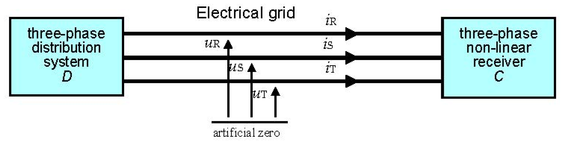
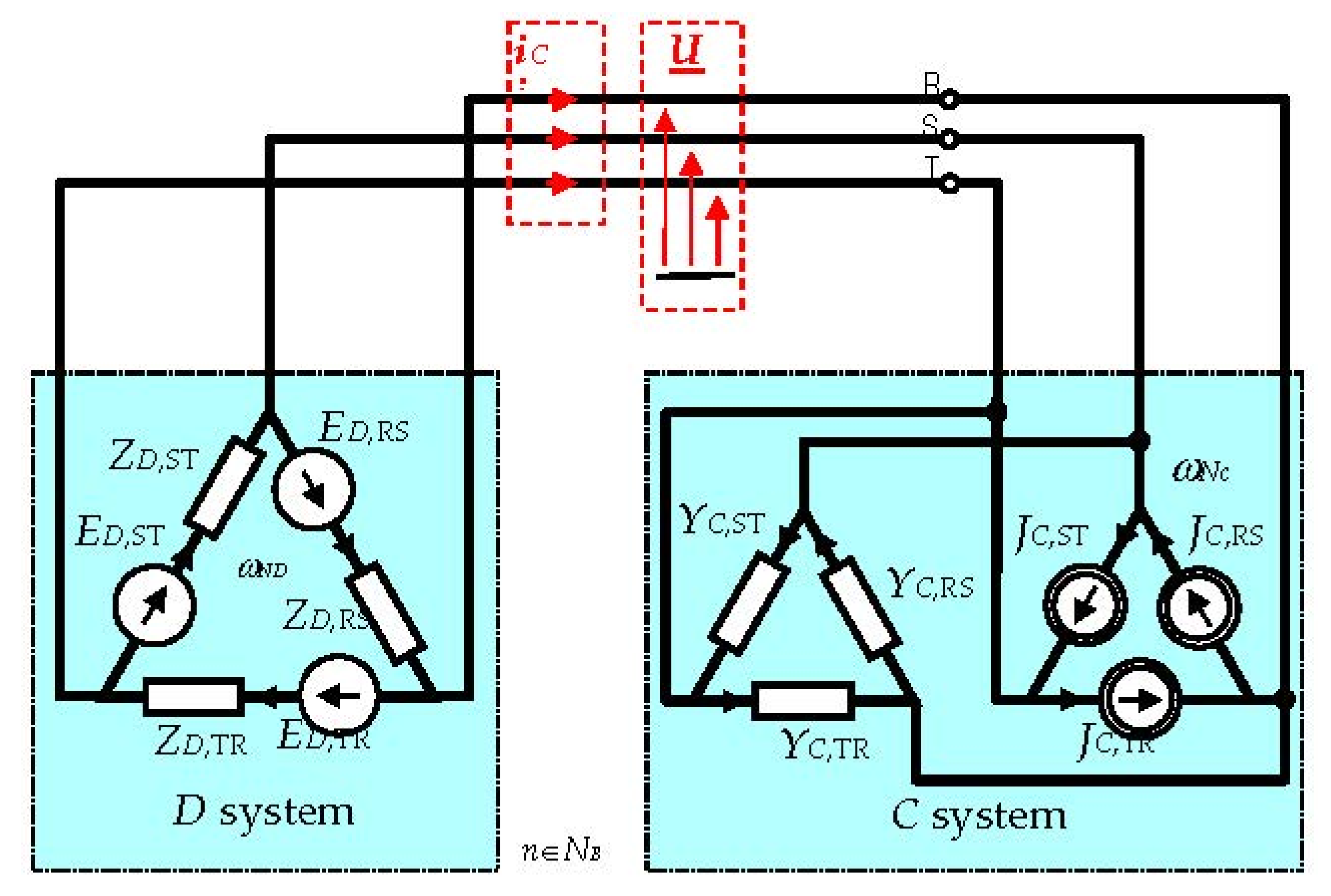
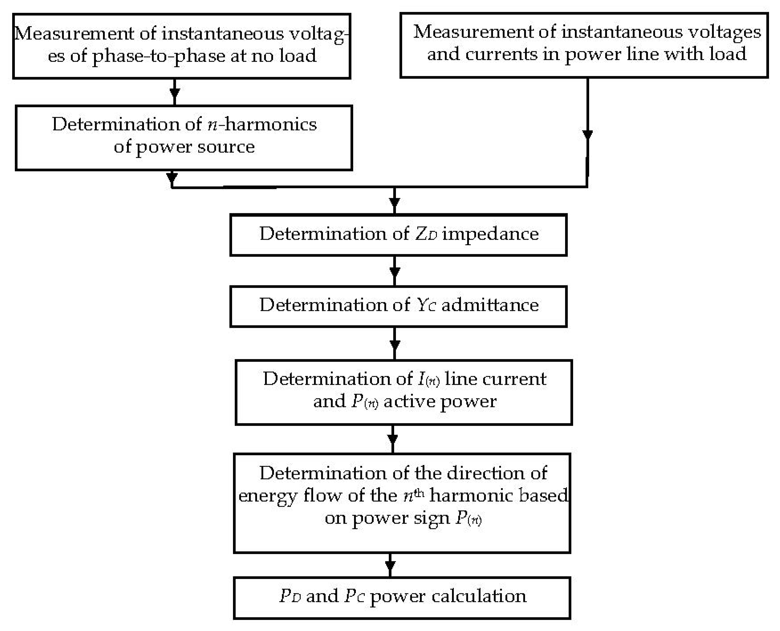
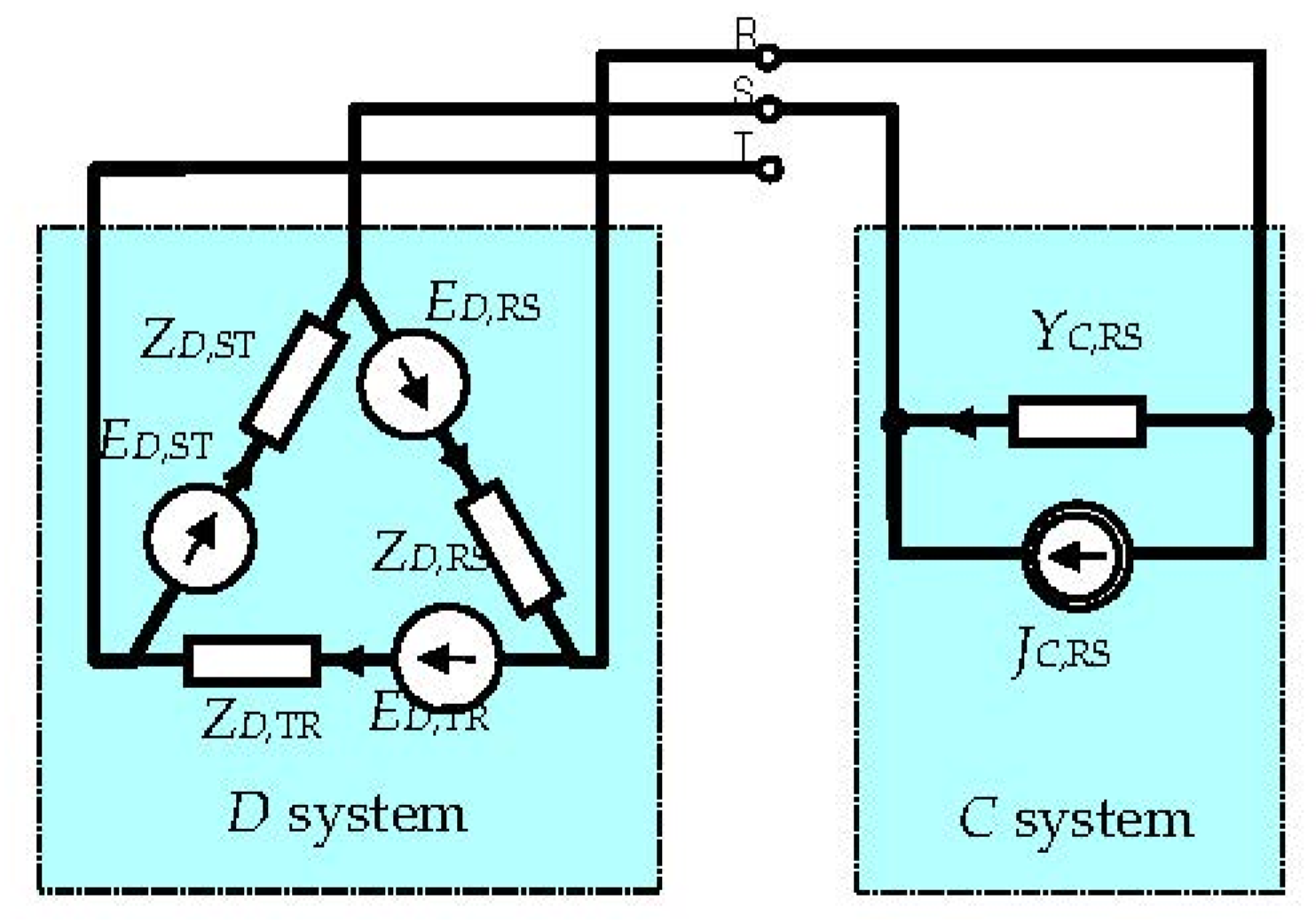
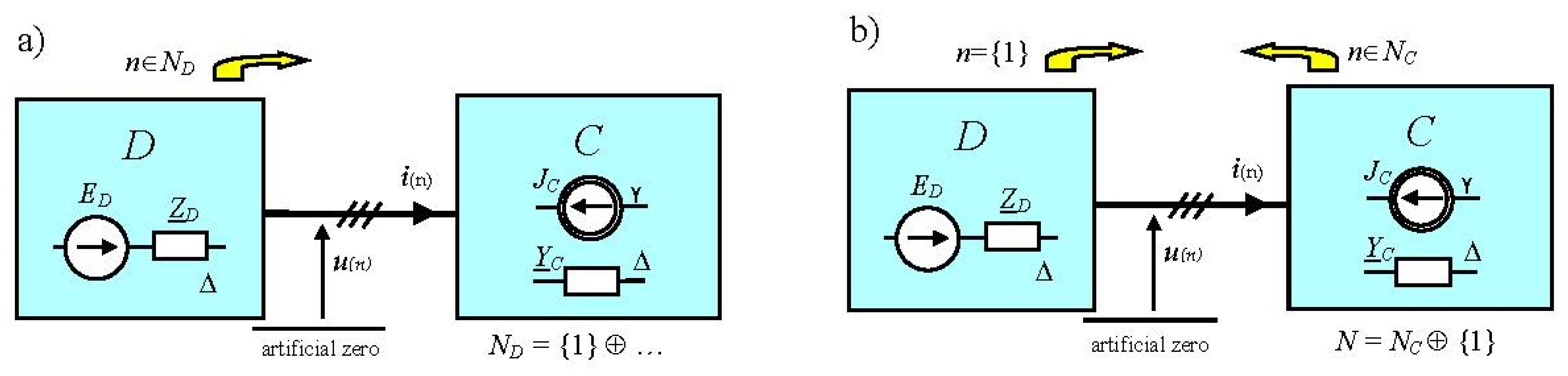
2. Mathematical Description of the Circuit

Energy phenomena accompanying the generation of harmonics by a non-linear receiver will be denoted by the “C” index, while those originating in the distribution system by the “D” index.

Both the source and the receiver are treated as black boxes in this study without the need to distinguish between Δ/Y topology. Only electrical quantities on the transmission line will be observed, with the reservation that the transmission line supplies electricity to the tested-only receiver. The description of the power and distribution of CPC currents will be possible by observing the instantaneous values of the line currents, i_R, i_S, and i_T, and the voltages, u_R, u_S, and u_T, relative to the virtual star point.

In the case of non-sinusoidal periodic waveforms, the direction of energy flow between the source and the receiver may be different for individual harmonics [16]. It will depend on the fact which of the C or D systems contributes to the generation of a given harmonic. It is r to consider the situation for each n-th harmonic separately. The set of all the harmonics present in the system (Figure 1) is marked with the N symbol. This set can be divided into N_D, the set of harmonics corresponding to the pulsations of the components describing the flow of energy from D to C system and N_C, the opposite flow.

The active power P_D(n) associated with the flow of energy from the source to the receiver is positive power, and P_C(n) associated with the opposite direction is negative power. The direction of a permanent energy transfer in a three-phase circuit is determined by examining the sign of the three-phase active power of the n-th harmonic P_(n).

$$P_{\left(n\right)}=U_{\mathrm{R}\left(n\right)}{I}_{\mathrm{R}\left(n\right)}\cos {\phi }_{\mathrm{R}\left(n\right)}+U_{\mathrm{S}\left(n\right)}{I}_{\mathrm{S}\left(n\right)}\cos {\phi }_{\mathrm{S}\left(n\right)}+U_{\mathrm{T}\left(n\right)}{I}_{\mathrm{T}\left(n\right)}\cos {\phi }_{\mathrm{T}\left(n\right)}$$

(1)

This approach assumes that the direction of energy flow for the n-th harmonic in all the phases is the same. If the directions of energy flow in individual phases are different, the three-phase active power P_(n) of the n-th harmonic will be the resultant power characterizing the three-phase power circuit.

According to the indexes adopted, the harmonics were divided into N_D and N_C sets.

$$\left.\begin{array}{ll}\hfill & P_{\left(n\right)}\ge 0\hfill \\ \hfill & P_{\left(n\right)}<0\hfill \end{array}\right\}\begin{array}{c}{P}_{D\left(n\right)}=P_{\left(n\right)}, n\in N_D\\ P_{C\left(n\right)}=-P_{\left(n\right)}, n\in N_C\end{array}$$

(2)

When the active power P_(n) for the n-th harmonic is positive, it should be assumed that it comes from the D system (Figure 2a), or the power P_D(n) produced by it dominates due to the direction of energy flow over the harmonic current of the same order generated in the receiver P_C(n). Otherwise, it is possible to isolate a set of N_C harmonics (Figure 2b).

Thus, the active power is divided into two powers [17]:

• P_D—working active power, generated by the E_D voltage source and transferred to the Y_C receiver admittance (Figure 2a), and
• P_C—reflective active power, generated by the J_C current source and transferred to the Z_D internal impedance of the D system (Figure 2b).

The P_D component has a positive value due to the flow of energy from the source to the receiver, while P_C has a negative value due to the change of the sign of the voltage U_(n), caused by the change in the direction of the current flowing through the R_C resistance.

The vectors of currents and voltages in the three-phase system shown in Figure 2 are defined in an instantaneous and complex vector form:

$${\mathit{u}}_{\left(n\right)}={\mathit{u}}_{\left(n\right)}\left(t\right)=\left[\begin{array}{c}{u}_{\mathrm{R}\left(n\right)}\\ u_{\mathrm{S}\left(n\right)}\\ u_{\mathrm{T}\left(n\right)}\end{array}\right]\hspace{1em}\hspace{1em}{\mathit{i}}_{\left(n\right)}={\mathit{i}}_{\left(n\right)}\left(t\right)=\left[\begin{array}{c}{i}_{\mathrm{R}\left(n\right)}\\ i_{\mathrm{S}\left(n\right)}\\ i_{\mathrm{T}\left(n\right)}\end{array}\right]$$

(3)

$${\underset{¯}{\mathit{U}}}_{\left(n\right)}=\left[\begin{array}{c}{\underset{¯}{\mathit{U}}}_{\mathrm{R}\left(n\right)}\\ {\underset{¯}{U}}_{\mathrm{S}\left(n\right)}\\ {\underset{¯}{U}}_{\mathrm{T}\left(n\right)}\end{array}\right]\hspace{1em}\hspace{1em}\hspace{1em}{\underset{¯}{U}}_{\left(n\right)}^{\#}=\left[\begin{array}{c}{\underset{¯}{U}}_{\mathrm{R}\left(n\right)}\\ {\underset{¯}{U}}_{\mathrm{T}\left(n\right)}\\ {\underset{¯}{U}}_{\mathrm{S}\left(n\right)}\end{array}\right]$$

(4)

The effective values (RMS) of the three-phase voltage and current are:

$$‖u‖=\sqrt{{\displaystyle \sum _{n=1}^N\left({‖u_{\mathrm{R}\left(n\right)}‖}^2+{‖u_{\mathrm{S}\left(n\right)}‖}^2+{‖u_{\mathrm{T}\left(n\right)}‖}^2\right)}}$$

(5)

$$‖i‖=\sqrt{{\displaystyle \sum _{n=1}^N\left({‖i_{\mathrm{R}\left(n\right)}‖}^2+{‖i_{\mathrm{S}\left(n\right)}‖}^2+{‖i_{\mathrm{T}\left(n\right)}‖}^2\right)}}$$

(6)

In a three-wire system, the sum of phase currents is equal to i_R + i_S + i_T = 0. The sum of the voltages u_R + u_S + u_T depends on the reference potential. The reference voltage added to each phase voltage changes the RMS value of the three-phase voltage, but it does not change the current and energy values. This means that Equation (5) is valid only in the case of:

$$u_{\mathrm{R}}+u_{\mathrm{S}}+u_{\mathrm{T}}=0$$

(7)

that is, phase voltages, due to orthogonality, cannot have zero-order components, i.e., n ≠ 3k + 3, k ∈ N. In practice, this condition is met because the secondary windings of transformers are usually connected in the Δ topology.

According to the CPC power theory [17], the three-phase three-wire system under examination should be decomposed into several components:

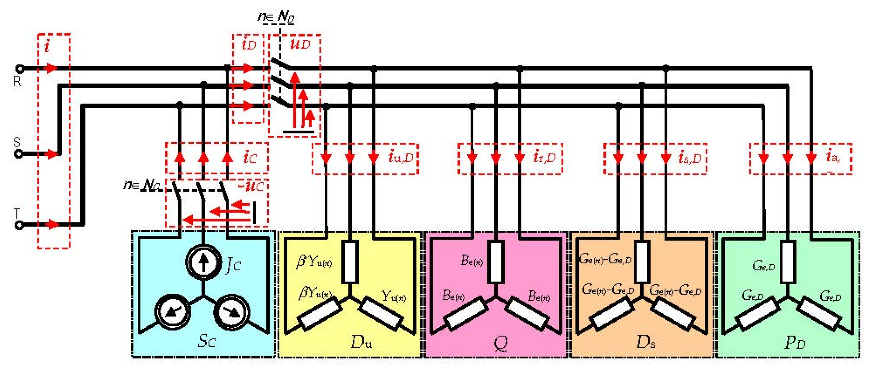
• vector i_a—the active component of the current, depending on the P active power of the receiver and, at the same time, on the resultant of the equivalent conductance G_e of the receiver. The value of this conductance describes a pure-resistive receiver, and it is directly proportional to the active power P and inversely proportional to the square of the RMS value of the voltage ${‖\mathit{u}‖}^2$. The instantaneous and effective value of this component is:

  $${\mathit{i}}_{\mathrm{a}}=\sqrt{2}\Re e\left\{G_{\mathrm{e}}\underset{¯}{\mathit{U}}{e}^{j{\omega }_{1}t}\right\}\hspace{1em}\hspace{1em}‖{\mathit{i}}_{\mathrm{a}}‖=G_{\mathrm{e}}‖\mathit{u}‖=\frac{P}{‖\mathit{u}‖}$$

  (8)
• vector i_s—the scattered component of current; it appears when the G_e(n) equivalent conductance of the receiver changes with the order of harmonics. The instantaneous and effective value of this component is:

  $${\mathit{i}}_{\mathrm{s}}=\sqrt{2}\Re e\left\{{\displaystyle \sum _n\left(G_{\mathrm{e}\left(n\right)}-G_{\mathrm{e}}\right)\cdot {\underset{¯}{\mathit{U}}}_{\left(n\right)}{e}^{jn{\omega }_{1}t}}\right\}\hspace{1em}\hspace{1em}‖{\mathit{i}}_{\mathrm{s}}‖=\sqrt{{\displaystyle \sum _n{\left(G_{\mathrm{e}\left(n\right)}-G_{\mathrm{e}}\right)}^2{‖{\mathit{u}}_{\left(n\right)}‖}^2}}$$

  (9)
• vector i_r—the reactive component of current; it appears when there is a non-zero phase shift between the vectors of current i_(n) and voltage u_(n), for any harmonic in any phase. The condition for this shift to exist is a non-zero equivalent susceptance B_e(n) ≠ 0.

  $${\mathit{i}}_{\mathrm{r}}=\sqrt{2}\Re e\left\{{\displaystyle \sum _{n}j{B}_{\mathrm{e}\left(n\right)}}{\underset{¯}{\mathit{U}}}_{\left(n\right)}{e}^{jn{\omega }_{1}t}\right\}\hspace{1em}\hspace{1em}‖{\mathit{i}}_{\mathrm{r}}‖=\sqrt{{\displaystyle \sum _n{B}_{\mathrm{e}\left(n\right)}^2{‖{\mathit{u}}_{\left(n\right)}‖}^2}}$$

  (10)
• vector i_u—the unbalanced component of current; it appears in the case of non-zero unbalanced admittance Y_u(n) ≠ 0.

  $${\mathit{i}}_{\mathrm{u}}=\sqrt{2}\Re e\left\{{\displaystyle \sum _n{\underset{¯}{Y}}_{\mathrm{u}\left(n\right)}}{\underset{¯}{\mathit{U}}}_{\left(n\right)}^{\#}{e}^{jn{\omega }_{1}t}\right\}\hspace{1em}\hspace{1em}‖{\mathit{i}}_{\mathrm{u}}‖=\sqrt{{\displaystyle \sum _n{Y}_{\mathrm{u}\left(n\right)}^2{‖{\mathit{u}}_{\left(n\right)}‖}^2}}$$

  (11)

The components above form together the vector of current flowing through the power line connecting the receiver with the source. The instantaneous value of this current is:

$$\mathit{i}={\mathit{i}}_{\mathrm{a}}+{\mathit{i}}_{\mathrm{s}}+{\mathit{i}}_{\mathrm{r}}+{\mathit{i}}_{\mathrm{u}}$$

(12)

while due to the mutual orthogonality of these components, the RMS value of the current is:

$${‖\mathit{i}‖}^2={‖{\mathit{i}}_{\mathrm{a}}‖}^2+{‖{\mathit{i}}_{\mathrm{s}}‖}^2+{‖{\mathit{i}}_{\mathrm{r}}‖}^2+{‖{\mathit{i}}_{\mathrm{u}}‖}^2$$

(13)

The two-sided multiplication of Equation (13) by the ${‖\mathit{u}‖}^2$ square of the RMS value of the voltage vector yields the power equation:

$$S^2=P^2+D_s^2+Q^2+D_u^2$$

(14)

where the individual components are:

• P—active power, W,
• S—apparent power, VA,
• Q—reactive power, var,
• D_u—unbalanced power, VA,
• D_s—scattered power, VA.

These powers have no physical interpretation. They are the result of multiplying the RMS values of the physical components of the current with the voltage. Even the P active power does not have its physical interpretation, because in these analyses, it cannot assume negative values. This is only valid for passive receivers.

The set of N harmonics includes the N_D and N_C subsets, which group the harmonics in terms of the direction of the energy flow of the n-th harmonic (n = 1…N) from the D to C system and from C to D, respectively (Figure 3).

In certain situations, a non-linear receiver can be expected to generate the same harmonics that have already existed in the power grid. In practical measurements, this condition is difficult to locate, and it is manifested by an increase in the amplitude of the n-th harmonic of the current after connecting a non-linear receiver. This is an important case when two non-linear receivers generating the same harmonic to a common power grid are considered. This group of harmonics is marked with the symbol N_B (both directions). In this group of harmonics, it is possible for energy to flow either in the direction from D to C or from C to D system.

The components related to the flow of energy from the source to the receiver are:

$${\mathit{i}}_D={\displaystyle \sum _{n\in N_D}{\mathit{i}}_{\left(n\right)}},\hspace{1em}\hspace{1em} {\mathit{u}}_D={\displaystyle \sum _{n\in N_D}{\mathit{u}}_{\left(n\right)}},\hspace{1em} P_D={\displaystyle \sum _{n\in N_D}{P}_{\left(n\right)}}$$

(15)

while with the opposite flow, these are:

$${\mathit{i}}_C={\displaystyle \sum _{n\in N_C}{\mathit{i}}_{\left(n\right)}},\hspace{1em} {\mathit{u}}_C=-{\displaystyle \sum _{n\in N_C}{\mathit{u}}_{\left(n\right)}},\hspace{1em} P_C=-{\displaystyle \sum _{n\in N_C}{P}_{\left(n\right)}}$$

(16)

In this way, the distribution of the components into two subsets was obtained, related to the direction of energy flow, which is a consequence of the physical phenomenon that caused it:

$$\mathit{i}={\mathit{i}}_D+{\mathit{i}}_C,\hspace{1em}\hspace{1em} \mathit{u}={\mathit{u}}_D-{\mathit{u}}_C,\hspace{1em}\hspace{1em} P=P_D-P_C$$

(17)

Due to the fact that the sets N_C and N_D are disjoint, the components above are mutually orthogonal, therefore:

$${‖\mathit{i}‖}^2={‖{\mathit{i}}_D‖}^2+{‖{\mathit{i}}_C‖}^2,\hspace{1em}\hspace{1em} {‖\mathit{u}‖}^2={‖{\mathit{u}}_D‖}^2+{‖{\mathit{u}}_C‖}^2,\hspace{1em}\hspace{1em} P^2=P_D^2+P_C^2$$

(18)

The active power at the receiver terminals, including the current and voltage, was decomposed into components related to the direction of the permanent energy flow.

The source–receiver interaction is considered by the superposition of both phenomena in the C and D systems analysed individually.

The energy flow from the source to the receiver is considered for harmonics belonging to the N_D set. The i_D component is described according to Formula (12):

$${\mathit{i}}_D={\mathit{i}}_{\mathrm{a},D}+{\mathit{i}}_{\mathrm{s},D}+{\mathit{i}}_{\mathrm{r},D}+{\mathit{i}}_{\mathrm{u},D}$$

(19)

including an equivalent admittance:

$$G_{\mathrm{e},D}=\frac{P_D}{{‖{\mathit{u}}_D‖}^2}$$

(20)

A comparison of Formulas (17) and (19) leads to:

$$\mathit{i}={\mathit{i}}_{\mathrm{a},D}+{\mathit{i}}_{\mathrm{s},D}+{\mathit{i}}_{\mathrm{r},D}+{\mathit{i}}_{\mathrm{u},D}+{\mathit{i}}_C$$

(21)

where the individual components and their RMS values are equal to:

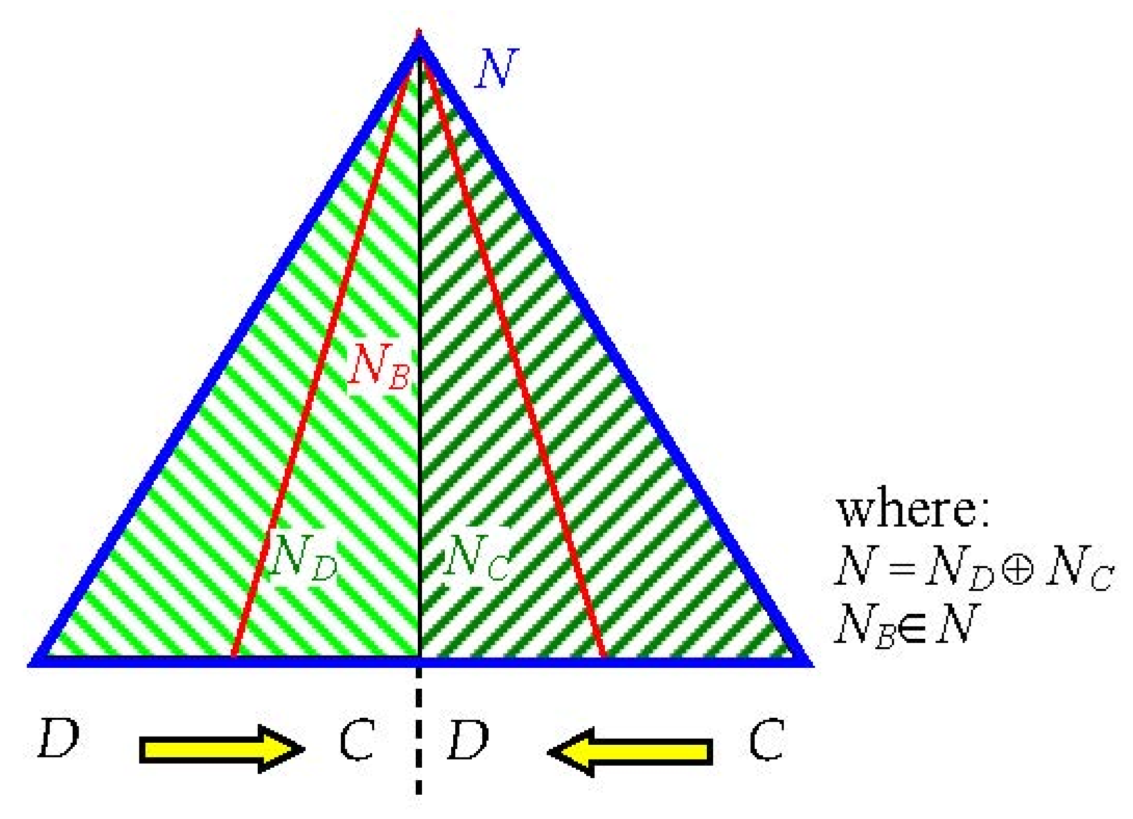
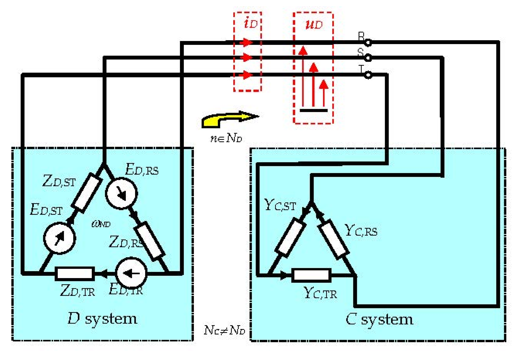
• vector of the active component of current for the direction from D to C:

$${\mathit{i}}_{\mathrm{a},D}=G_{\mathrm{e},D}\cdot {\mathit{u}}_D,\hspace{1em}\hspace{1em} ‖{\mathit{i}}_{\mathrm{a},D}‖=\frac{P_D}{‖{\mathit{u}}_D‖}$$

(22)

• vector of the scattered component of current for the direction from D to C:

$${\mathit{i}}_{\mathrm{s},D}=\sqrt{2}\Re e\left\{{\displaystyle \sum _{n\in N_D}\left(G_{\mathrm{e}\left(n\right)}-G_{\mathrm{e},D}\right)\cdot {\underset{¯}{\mathit{U}}}_{\left(n\right)}\cdot e^{jn{\omega }_{1}t}}\right\},\hspace{1em}\hspace{1em} ‖{\mathit{i}}_{\mathrm{s},D}‖=\sqrt{{\displaystyle \sum _{n\in N_D}{\left(G_{\mathrm{e}\left(n\right)}-G_{\mathrm{e},D}\right)}^2{‖{\mathit{u}}_{\left(n\right)}‖}^2}}=\frac{D_s}{‖{\mathit{u}}_D‖}$$

(23)

• vector of the reactive component of current for the direction from D to C:

$${\mathit{i}}_{\mathrm{r},D}=\sqrt{2}\Re e\left\{{\displaystyle \sum _{n\in N_D}j{B}_{\mathrm{e}\left(n\right)}\cdot {\underset{¯}{\mathit{U}}}_{\left(n\right)}\cdot e^{jn{\omega }_{1}t}}\right\},\hspace{1em}\hspace{1em} ‖{\mathit{i}}_{\mathrm{r},D}‖=\sqrt{{\displaystyle \sum _{n\in N_D}{B}_{\mathrm{e}\left(n\right)}^2{‖{\mathit{u}}_{\left(n\right)}‖}^2}}=\frac{Q}{‖{\mathit{u}}_D‖}$$

(24)

• vector of the unbalanced component of current for the direction from D to C:

$${\mathit{i}}_{\mathrm{u},D}=\sqrt{2}\Re e\left\{{\displaystyle \sum _{n\in N_D}{\underset{¯}{Y}}_{\mathrm{u}\left(n\right)}\cdot {\underset{¯}{\mathit{U}}}_{\left(n\right)}^{\#}\cdot e^{jn{\omega }_{1}t}}\right\},\hspace{1em}\hspace{1em} ‖{\mathit{i}}_{\mathrm{u},D}‖=\sqrt{{\displaystyle \sum _{n\in N_D}{Y}_{\mathrm{u}\left(n\right)}^2{‖{\mathit{u}}_{\left(n\right)}‖}^2}}=\frac{D_u}{‖{\mathit{u}}_D‖}$$

(25)

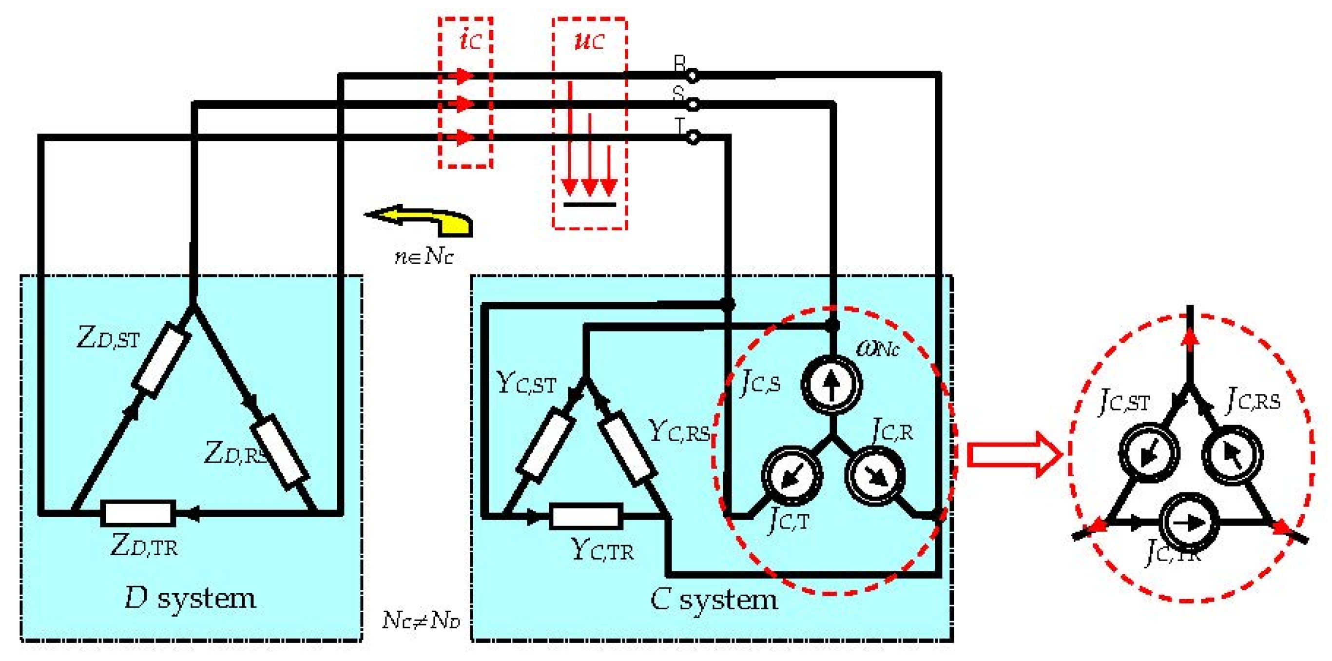
• vector of the component of current generated by the non-linear receiver for the direction from C to D:

$${\mathit{i}}_C=\sqrt{2}\Re e\left\{{\displaystyle \sum _{n\in N_C}{\underset{¯}{\mathit{I}}}_{\left(n\right)}\cdot e^{jn{\omega }_{1}t}}\right\},\hspace{1em}\hspace{1em}\hspace{1em} ‖{\mathit{i}}_C‖=\sqrt{{\displaystyle \sum _{n\in N_C}{‖{\mathit{i}}_{\left(n\right)}^{}‖}^2}}=\frac{S_C}{‖{\mathit{u}}_C‖}$$

(26)

All these components are mutually orthogonal, so the following is correct:

$${‖\mathit{i}‖}^2={‖{\mathit{i}}_{\mathrm{a},D}‖}^2+{‖{\mathit{i}}_{\mathrm{s},D}‖}^2+{‖{\mathit{i}}_{\mathrm{r},D}‖}^2+{‖{\mathit{i}}_{\mathrm{u},D}‖}^2+{‖{\mathit{i}}_C‖}^2$$

(27)

A graphical interpretation of this equation is shown in Figure 4.

For the dominant direction of energy flow from D to C, the apparent power S_D according to (14) is:

$$S_D=‖{\mathit{u}}_D‖\cdot ‖{\mathit{i}}_D‖=\sqrt{P_D^2+D_s^2+Q^2+D_u^2}$$

(28)

while for the opposite direction, the apparent power S_C has the following value:

$$S_C=‖{\mathit{u}}_C‖\cdot ‖{\mathit{i}}_C‖$$

(29)

The total apparent power of the system can be represented as follows:

$$S^2={‖\mathit{u}‖}^2{‖\mathit{i}‖}^2=\left({‖{\mathit{u}}_D‖}^2+{‖{\mathit{u}}_C‖}^2\right)\cdot \left({‖{\mathit{i}}_D‖}^2+{‖{\mathit{i}}_C‖}^2\right)=\underset{S_D^2}{\underbrace{{‖{\mathit{u}}_D‖}^2{‖{\mathit{i}}_D‖}^2}}+\underset{S_{DC}^2}{\underbrace{{‖{\mathit{u}}_D‖}^2{‖{\mathit{i}}_C‖}^2+{‖{\mathit{u}}_C‖}^2{‖{\mathit{i}}_D‖}^2}}+\underset{S_C^2}{\underbrace{{‖{\mathit{u}}_C‖}^2{‖{\mathit{i}}_C‖}^2}}$$

(30)

The mutual combination of the systems C and D is described by the resultant power S_DC:

$$S_{DC}=\sqrt{{‖{\mathit{u}}_D‖}^2{‖{\mathit{i}}_C‖}^2+{‖{\mathit{u}}_C‖}^2{‖{\mathit{i}}_D‖}^2}$$

(31)

In this case, the power equation is:

$$S^2=P_D^2+D_{\mathrm{s}}^2+Q_{}^2+D_u^2+S_C^2+S_{DC}^2$$

(32)

where the active power is equal:

$$P=P_D-P_C$$

(33)

With this approach, the power factor is:

$$\lambda =\frac{P}{S}=\frac{P_D-P_C}{\sqrt{P_D^2+D_{\mathrm{s}}^2+Q_{}^2+D_{\mathrm{u}}^2+S_C^2+S_{DC}^2}}$$

(34)

Both cases should be analysed separately, paying particular attention to the direction of the energy flow. Determination of the equations describing the phenomena of energy flow in particular directions must be carried out as follows:

(a)

for the flow of energy from a non-linear receiver to the source

Harmonics of current i_C caused by the source J_C of a given phase affect the passive inductor with impedance Z_D (Figure 5). This interaction gives rise to a potential difference for phase x, where x = {RS, ST, TR} is:

$${\underset{¯}{U}}_{C,x\left(n\right)}=\frac{{\underset{¯}{J}}_{C,x\left(n\right)}\cdot {\underset{¯}{Z}}_{D,x\left(n\right)}}{1+{\underset{¯}{Y}}_{C,x\left(n\right)}\cdot {\underset{¯}{Z}}_{D,x\left(n\right)}},\hspace{1em}\mathrm{for}n\in N_C$$

(35)

where the values of the phase current sources are related to the equivalent phase-to-phase sources according to the following complex relations:

$$\left\{\begin{array}{c}{\underset{¯}{J}}_{C,\mathrm{R}}={\underset{¯}{J}}_{C,\mathrm{TR}}-{\underset{¯}{J}}_{C,\mathrm{RS}}\\ {\underset{¯}{J}}_{C,\mathrm{S}}={\underset{¯}{J}}_{C,\mathrm{RS}}-{\underset{¯}{J}}_{C,\mathrm{ST}}\\ \hspace{1em} 0={\underset{¯}{J}}_{C,\mathrm{RS}}+{\underset{¯}{J}}_{C,\mathrm{ST}}+{\underset{¯}{J}}_{C,\mathrm{TR}}\end{array}\right.$$

(36)

The solution to Equation (36) is:

$$\left\{\begin{array}{c}{\underset{¯}{J}}_{C,\mathrm{RS}}=\frac{1}{3}{\underset{¯}{J}}_{C,\mathrm{S}}-\frac{1}{3}{\underset{¯}{J}}_{C,\mathrm{R}}\hfill \\ {\underset{¯}{J}}_{C,\mathrm{ST}}=-\frac{2}{3}{\underset{¯}{J}}_{C,\mathrm{S}}-\frac{1}{3}{\underset{¯}{J}}_{C,\mathrm{R}}\hfill \\ {\underset{¯}{J}}_{C,\mathrm{TR}}=\frac{1}{3}{\underset{¯}{J}}_{C,\mathrm{S}}+\frac{2}{3}{\underset{¯}{J}}_{C,\mathrm{R}}\hfill \end{array}\right.$$

(37)

(b)

for the flow of energy from the source to the non-linear receiver

Harmonics of current i_D caused by the source E_D of a given phase affect the passive admittance Y_C (Figure 6). The potential difference for phase x is:

$${\underset{¯}{U}}_{D,x\left(n\right)}=\frac{{\underset{¯}{E}}_{D,x\left(n\right)}}{1+{\underset{¯}{Y}}_{C,x\left(n\right)}\cdot {\underset{¯}{Z}}_{D,x\left(n\right)}},\hspace{1em}\mathrm{for}n\in N_D$$

(38)

Taking into account the possibility of overlapping harmonics in the waveforms: E_D power source and those generated by the non-linear receiver J_C, the full form of the diagram should be considered (Figure 7).

Harmonics occurring simultaneously both in E_D and J_C sources are characterized by the possibility of energy transmission in both directions. For the set of N_B harmonics, for phase x, the following relationship will be valid:

$${\underset{¯}{U}}_{x\left(n\right)}=\frac{{\underset{¯}{E}}_{D,x\left(n\right)}-{\underset{¯}{J}}_{C,x\left(n\right)}\cdot {\underset{¯}{Z}}_{D,x\left(n\right)}}{1+{\underset{¯}{Y}}_{C,x\left(n\right)}\cdot {\underset{¯}{Z}}_{D,x\left(n\right)}},\hspace{1em}\mathrm{for}n\in N_B$$

(39)

where the current sources are described by Relations (37). The relationship between the phase voltages of the source and receiver connected in the Δ topology and the line voltages is as follows:

$$\left\{\begin{array}{c}{\underset{¯}{U}}_{\mathrm{TR}}={\underset{¯}{U}}_{\mathrm{T}}-{\underset{¯}{U}}_{\mathrm{R}}\\ {\underset{¯}{U}}_{\mathrm{RS}}={\underset{¯}{U}}_{\mathrm{R}}-{\underset{¯}{U}}_{\mathrm{S}}\\ \hspace{1em}0={\underset{¯}{U}}_{\mathrm{R}}+{\underset{¯}{U}}_{\mathrm{S}}+{\underset{¯}{U}}_{\mathrm{T}}\end{array}\right.$$

(40)

As a result of solving Equation (40), we obtain:

$$\left\{\begin{array}{l}{\underset{¯}{U}}_{\mathrm{R}}=\frac{1}{3}{\underset{¯}{U}}_{\mathrm{RS}}-\frac{1}{3}{\underset{¯}{U}}_{\mathrm{TR}}\hfill \\ {\underset{¯}{U}}_{\mathrm{S}}=-\frac{2}{3}{\underset{¯}{U}}_{\mathrm{RS}}-\frac{1}{3}{\underset{¯}{U}}_{\mathrm{TR}}\hfill \\ {\underset{¯}{U}}_{\mathrm{T}}=\frac{1}{3}{\underset{¯}{U}}_{\mathrm{RS}}+\frac{2}{3}{\underset{¯}{U}}_{\mathrm{TR}}\hfill \end{array}\right.$$

(41)

The proposed method of analysis can be presented in a block form (Figure 8).

The method of defining the voltage and current vectors and the method of determining the N_C and N_D harmonic sets impose a limitation to the class of non-linear receivers, in which non-linearities behave identically for each phase. This means that the method presented is correct only in the case of a consistent direction of energy flow in each phase for any harmonic considered individually.

In addition, it should be remembered that the distribution presented of the CPC current components for non-linear three-phase circuits (27) is a form of an approximation of the phenomena caused by two three-phase sources, which were reduced to the resultant voltage $\mathit{u}={\mathit{u}}_D-{\mathit{u}}_C$, depending on the direction of energy flow. As a result, the use of this method requires special attention.

It is also significant that in practice, a change in the supply voltage e_D results in a change in the parameters of the current source J_C of the non-linear receiver. The parameter J_C is actually a function depending on the value of the voltage u. The actual state of the non-linear system is based on the functional dependence of the parameters of the non-linear receiver on the operating point. Thus, this distribution is true only at a specific operating point.

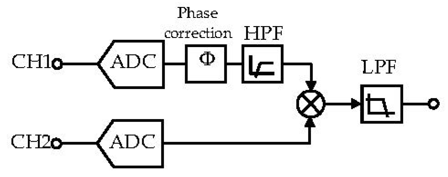
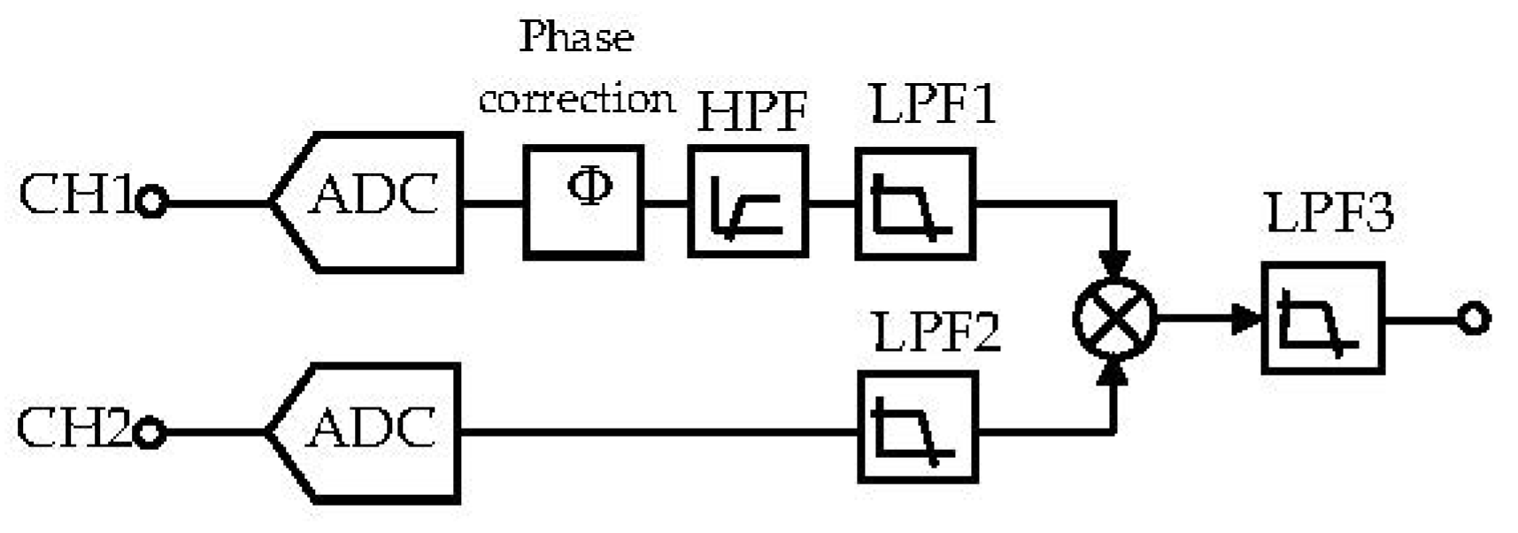
3. Electronic Measuring Methods of Active Power

Modern power/energy measuring methods are based on an electronic measurement of current and voltage waveforms and the use of appropriate algorithms [23]. When analysing the applications used by the individual manufacturers of electricity meters, several calculation methods can be presented.

3.1. Calculation of Active Power Resulting from an Analysis of the Waveform of the Instantaneous Power Signal

The active power is determined according to the following relation:

$$P=\frac{1}{kT}{\displaystyle \underset{\tau }{\overset{\tau +kT}{\int }}u\left(t\right)\cdot i\left(t\right)dt}$$

(42)

where: T—period, k—number of periods to be averaged

First, the instantaneous values of voltage u and current i are multiplied. The integration operation is often replaced by summing the rectangles under the power function. In this way, the average power value is obtained, which in this case is treated as active power. The result of this action in the light of Emanuel’s theory [24] is the value:

$$P=P_1+P_{\mathrm{H}}$$

(43)

where:

-

fundamental component of the active power

$$P_1=\frac{1}{kT}{\displaystyle \underset{\tau }{\overset{\tau +kT}{\int }}{u}_1{i}_{1}dt}=U_1{I}_1\cos {\theta }_1\left[\mathrm{W}\right]$$

(44)

-

harmonic component of the active power

$$P_{\mathrm{H}}=U_0{I}_0+{\displaystyle \sum _{h\ne 1}{U}_{\left(h\right)}{I}_{\left(h\right)}\cos {\theta }_{\left(h\right)}}\left[\mathrm{W}\right]$$

(45)

3.2. Determination of Individual Powers from Basic Power Equations for Sinusoidal Waveforms

The principle of this method is to determine the value of the phase shift, as well as the RMS values of current and voltage. In this method, to determine the active power component, the instantaneous power of the signal is filtered with the Low Pass Filter (LPF) (Figure 9).

This measurement method correctly calculates the active power also for non-sinusoidal current and voltage waveforms for any power factor value. The entire signal processing algorithm takes place on the digital side, so it is devoid of any interference caused by the influence of temperature and time. The harmonic component of the active power generated for each harmonic is determinable when harmonics are present both in the current and voltage waveforms.

3.3. Measurement of Fundamental Component of the Active Power

This method may use the computational capabilities of microcontrollers. Their task is to collect current and voltage measurement samples in a given period of time. The Fast Fourier Transform (FFT) can be used to determine the fundamental components u₁ and i₁ (46).

$$u_1=U_{\left(1\right)}\sqrt{2}\sin \left({\omega }_{1}t+{\alpha }_{\left(1\right)}\right),\hspace{1em}\hspace{1em} i_1=I_{\left(1\right)}\sqrt{2}\sin \left({\omega }_{1}t+{\alpha }_{\left(1\right)}\right)$$

(46)

Numerical integration can be performed using the trapezoidal method to increase accuracy. This method approximates the calculated function with a straight line passing through the boundary points of the interval. Determination of the fundamental components can be carried out by applying low-pass filtering in both measurement channels (Figure 10).

The effect of the High Pass Filter (HPF) on channel 1 shifts the phase of this signal. To reduce this error and balance the phase response between CH1 and CH2, a phase correction was placed in CH1. The LPF1 and LPF2 filters transfer the fundamental components of current and voltage. The LPF3 filter transfers only the constant component of the multiplication operation u₁ ∙ i₁, which corresponds to the value of the active power of the fundamental component P₁. Instead of the LPF1 and LPF2 filters, Kalman filters can be made, whose task will be to approximate the waveforms measured to Form (46).

4. Example and Discussion

A single-phase non-linear receiver was connected to a symmetrical three-phase source whose internal impedance Z_D consists of resistance R_D = 0.01 Ω and inductance L_D = 0.5/π mH (Figure 11). The source pulsation is ω = 2π50 rad/s, while a symmetrical three-phase voltage source is equal to:

$$e_{\mathrm{RS}}=\sqrt{2}\left[230\sin \left(\omega t\right)+80\sin \left(2\omega t\right)+30\sin \left(5\omega t\right)\right] \mathrm{V},$$

$$e_{\mathrm{TR}}=\sqrt{2}\left[230\sin \left(\omega t+\frac{2\pi }{3}\right)+80\sin \left(2\omega t+2\frac{2\pi }{3}\right)+30\sin \left(5\omega t+5\frac{2\pi }{3}\right)\right] \mathrm{V},$$

$$e_{\mathrm{ST}}=\sqrt{2}\left[230\sin \left(\omega t+\frac{4\pi }{3}\right)+80\sin \left(2\omega t+2\frac{4\pi }{3}\right)+30\sin \left(5\omega t+5\frac{4\pi }{3}\right)\right] \mathrm{V}.$$

The non-linear receiver has resistance R_C = 0.1 Ω and inductance L_C = 0.001/π H, and it generates current harmonics $j_{\mathrm{RS}}=\sqrt{2}\left[10\sin \left(2\omega t\right)+2\sin \left(7\omega t\right)\right] \mathrm{A}$ to the network.

The calculation results are presented in

Table 1. Impedances and admittances of C and D systems.

n	1	2	5	7
${\underset{¯}{Z}}_{D\left(n\right)}=R_D+jn\omega L_D$ [Ω]	0.01 + j0.05	0.01 + j0.1	0.01 + j0.25	0.01 + j0.35
${\underset{¯}{Y}}_{C,\mathrm{RS}\left(n\right)}=\frac{1}{R_C+jn\omega L_C}$ [S]	5 − j5	2 − j4	0.3846 − j1.9231	0.2 − j1.4

and

Table 2. Voltages, currents and powers.

n	1 ∈ ND	2 ∈ NB	5 ∈ ND	7 ∈ NC
URS [V]	172.83 − j26.59	55.48 − j6.96	20.15 − j1.04	0.03 − j0.47
IR [A]	731.21 − j997.11	−93.14 + j235.85	5.74 − j39.16	−2.66 − j0.05
PRS [W]	152.89∙103	−6.81∙103	156.63	−0.11

.

The first and fifth harmonics occur only in the D system, so Equation (38) will be used for them, Equation (35) for the seventh harmonic, and Equation (39) for the second harmonic.

Where the line current is equal to: ${\underset{¯}{I}}_{\mathrm{R}\left(n\right)}=\left\{\begin{array}{ll}{\underset{¯}{U}}_{\mathrm{RS}\left(n\right)}{\underset{¯}{Y}}_{C,\mathrm{RS}\left(n\right)}\hfill & \mathrm{for} n\in N_D,\hfill \\ -\left({\underset{¯}{U}}_{\mathrm{RS}\left(n\right)}{\underset{¯}{Y}}_{C,\mathrm{RS}\left(n\right)}+{\underset{¯}{J}}_{C,\mathrm{RS}\left(n\right)}\right)\hfill & \mathrm{for} n\notin N_D,\hfill \end{array}\right.$

While the active power is equal to: $P_{\mathrm{RS}\left(n\right)}=\Re e\left\{{\underset{¯}{U}}_{\mathrm{RS}\left(n\right)}{\underset{¯}{I}}_{\mathrm{R}\left(n\right)}^{*}\right\}$

For the second harmonic, negative active power is obtained, which means that for this harmonic, the direction of energy flow is from the non-linear receiver to the source. Active powers according to Formulas (15) and (16) are as follows:

P_D = P_RS(1) + P_RS(5) = 153.05 kW,

P_C = –(P_RS(2) + P_RS(7)) = 6808.63 W,

P = P_D − P_C = 146.24 kW.

It is a well-known fact that active power is the power responsible for the effective part of the electricity that the receiver actively uses for energy transformations. However, not every receiver is able to use the energy transferred in higher harmonics. For example, AC motors actively use only the fundamental energy (in this example, P₁ = 152.89 kW). The remaining harmonics act unfavourably, causing disturbances in the rotating magnetic flux, which translates into a deterioration of efficiency. According to (45), active power that is not actively used in the receiver in this example is: $P_{\mathrm{H}}={\displaystyle \sum _{n\ne 1}\left|P_n\right|=}6.97 \mathrm{kW}$, which is 4.4% of the total power P₁ + P_H = 159.86 kW. Assuming a proportional relationship between the motor torque and its power, this means a 4.4% decrease in torque, even though the fee for active energy consumption will be charged on the total power of P₁ + P_H.

The situation is different in the case of resistive receivers. For example, an electric heater, in which the reactance character can be omitted, will convert electrical energy carried by all harmonics (in this example P = 146.24 kW). Two situations can be analysed: 1. The nonlinear receiver is powered by an individual electricity meter—in this case, the fee for the active energy consumed will be charged, the same as that flowed through the receiver, i.e., 159.86 kW. 2. The electricity meter supplies several receivers—in this situation, power P_C will be transferred between the receivers, and the electricity meter will register power P_D only. The indication will be underestimated by a value equal to P_C, which is 4.26% of the total power.

From the perspective of the electricity supplier, this is the most advantageous billing method for the consumed active power according to Time Dependence (42). Unfortunately, this is not a beneficial solution for all electricity consumers.

In addition, the definition of apparent power in three-phase circuits is not unambiguous. In three-phase circuits, there are several definitions of apparent power [25,26]. A three-phase circuit can be described by the apparent power determined according to Bucholz [27]:

$$\sqrt{U_{\mathrm{R}}^2+U_{\mathrm{S}}^2+U_{\mathrm{T}}^2}\cdot \sqrt{I_{\mathrm{R}}^2+I_{\mathrm{S}}^2+I_{\mathrm{T}}^2}=S_{Bu}$$

(47)

which, in this example, is: $S_{Bu}=\sqrt{{\displaystyle \sum _{n=1}^N{\left|{\underset{¯}{U}}_{\mathrm{RS}\left(n\right)}\right|}^2}}\cdot \sqrt{{\displaystyle \sum _{n=1}^N{\left|{\underset{¯}{I}}_{\mathrm{R}\left(n\right)}\right|}^2}}=233.2 \mathrm{kVA}$

The complex power is determined by the following relation:

$$\underset{¯}{S}={\underset{¯}{U}}_{\mathrm{R}}{\underset{¯}{I}}_{\mathrm{R}}^{*}+{\underset{¯}{U}}_{\mathrm{S}}{\underset{¯}{I}}_{\mathrm{S}}^{*}+{\underset{¯}{U}}_{\mathrm{T}}{\underset{¯}{I}}_{\mathrm{T}}^{*}$$

(48)

while its direction is consistent with the direction of active power. The length of this power vector is called the geometric apparent power [28], which in this example is:

$$S_G=\left|\underset{¯}{S}\right|=\left|{\displaystyle \sum _{n=1}^N\left({\underset{¯}{U}}_{\mathrm{RS}\left(n\right)}{\underset{¯}{I}}_{\mathrm{R}\left(n\right)}^{*}\right)}\right|=203.3 \mathrm{kVA}$$

In electronic energy meters, apparent power is measured in each phase individually; then, the final result is presented in the form of their sum. This power is called the arithmetic apparent power, and it is equal to:

$$S_{\mathrm{R}}+S_{\mathrm{S}}+S_{\mathrm{T}}=U_{\mathrm{R}}{I}_{\mathrm{R}}+U_{\mathrm{S}}{I}_{\mathrm{S}}+U_{\mathrm{T}}{I}_{\mathrm{T}}=S_{Ar}$$

(49)

When only one phase is loaded, this power is equal to the power according to Bucholz, determined from Relationship (47), S_Ar = S_Bu = 233.2 kVA.

The power measured by the electricity meter is an overestimated value in relation to the geometric power S_Ar > S_G. The summation of the scalar lengths of the three vectors will be greater than the length of the vector resulting from the addition of the three vectors.

Which quantities should be recognized in settlements? Standardization provides answers to these questions [29]. Despite many arguments and disagreements between the authors of the power theory, it should be emphasized that the superior method of electricity billing should be a unified system implemented by all the entities involved in the production, trade and consumption of electricity.

5. Conclusions

The analysis carried out in Section 4 allowed for a discussion on the methods of billing for the active power consumed. In a situation where higher harmonics appear, some consumers may be billed with an error of up to several percent.

According to [16], apparent power S and the power factor are conventional values that cannot be directly justified by physical characteristics. Nevertheless, the power factor is closely related to energy losses in the power system. Lowering the value of the power factor causes an increase in transmission losses. For this reason, it is proposed to choose the definition of apparent power—paying particular attention to an assessment of these losses.

In papers [15,18], an analysis of power factor values was carried out for the individual definitions of the apparent power in an unbalanced three-phase circuit. These analyses were focused on the correctness of the assessment of losses of transmission energy. The conclusion from the analyses conducted is that these losses are correctly estimated for the power factor calculated from apparent power according to the Buchholz theory. This definition is an extension of the definition of apparent power in single-phase circuits. This choice of the apparent power definition results in a failure to meet the power balance equation for an unbalanced three-phase circuit. In this case, the relation will be S² > P² + Q². Therefore, in billing for consumed reactive power, it is more advantageous to use inactive power, which includes all of those components that do not actively participate in energy transformations.

The analysis method based on the knowledge of J_C source parameters may be debatable. Determining these parameters may in fact be troublesome. The parameters of the J_C source depend on the values of other elements in the circuit and have an implicit functional dependence on other parameters: D system, power grid impedance, C system impedance and other harmonics. For this reason, the parameters of the J_C source are not stationary, and their values change as a result of changes in any other parameter in the circuit.

The ambiguity in the description of the electric circuit in various power theories results from the lack of a comprehensive mathematical description of the power system. Therefore, research in this area is still justified and needed.

It should be emphasized that the overriding method of electricity billing should be a unified system implemented by all the entities involved in the production, trade and consumption of electricity.

References

1. Smyczek, J.; Zajkowski, K. Simulation of overvoltages for switching off lagging load from mains. In Proceedings of the 2nd International Industrial Simulation Conference 2004, Malaga, Spain, 7–9 June 2004; pp. 278–281. [Google Scholar]
2. Zajkowski, K. Two-stage reactive compensation in a three-phase four-wire systems at nonsinusoidal periodic waveforms. Electr. Power Syst. Res. 2020, 184, 106296. [Google Scholar] [CrossRef]
3. Zajkowski, K. An innovative hybrid insulation switch to enable/disable electrical loads without overvoltages. In Proceedings of the International Conference Energy, Environment and Material Systems (EEMS 2017), E3S Web of Conferences, Polanica Zdrój, Poland, 13–15 September 2017; Volume 19. [Google Scholar] [CrossRef]
4. Zajkowski, K.; Rusica, I. The method of calculating LC parameters of balancing compensators in a three-phase four-wire circuit for an unbalanced linear receiver. In IOP Conference Series: Materials Science and Engineering, Proceedings of the Innovative Manufacturing Engineering and Energy (IManEE 2019)—"50 Years of Higher Technical Education at the University of Pitesti"—The 23rd Edition of IManEE 2019 International Conference, 22–24 May 2019, Pitesti, Romania; IOP Publishing Ltd.: Bristol, UK, 2019; Volume 564, p. 12134. [Google Scholar] [CrossRef]
5. Duer, S.; Zajkowski, K.; Scaticailov, S.; Wrzesień, P. Analyses of the method development of decisions in an expert system with the use of information from an artificial neural network. In Proceedings of the 22nd International Conference on Innovative Manufacturing Engineering and Energy—IManE&E 2018, MATEC Web of Conferences, Chisinau, Republic of Moldova, 31 May–2 June 2018. [Google Scholar] [CrossRef]
6. Duer, S.; Zajkowski, K.; Harničárová, M.; Charun, H.; Bernatowicz, D. Examination of Multivalent Diagnoses Developed by a Diagnostic Program with an Artificial Neural Network for Devices in the Electric Hybrid Power Supply System “House on Water”. Energies 2021, 14, 2153. [Google Scholar] [CrossRef]
7. Duer, S.; Rokosz, K.; Zajkowski, K.; Bernatowicz, D.; Ostrowski, A.; Woźniak, M.; Iqbal, A. Intelligent Systems Supporting the Use of Energy Devices and Other Complex Technical Objects: Modeling, Testing, and Analysis of Their Reliability in the Operating Process. Energies 2022, 15, 6414. [Google Scholar] [CrossRef]
8. Krzykowski, M.; Paś, J.; Rosiński, A. Assessment of the level of reliability of power supplies of the objects of critical infrastructure. IOP Conf. Ser. Earth Environ. Sci. 2019, 214, 012018. [Google Scholar] [CrossRef]
9. Siergiejczyk, M.; Pas, J.; Rosinski, A. Modeling of Process of Maintenance of Transport Systems Telematics with Regard to Electromagnetic Interferences. In Tools of Transport Telematics, Proceedings of the 15th International Conference on Transport Systems Telematics, TST 2015, Wrocław, Poland, 15–17 April 2015; Communications in Computer and Information Science; Mikulski, J., Ed.; Springer: Berlin/Heidelberg, Germany, 2015; Volume 531, pp. 99–107. [Google Scholar] [CrossRef]
10. Siergiejczyk, M.; Pas, J.; Rosinski, A. Issue of reliability–exploitation evaluation of electronic transport systems used in the railway environment with consideration of electromagnetic interference. IET Intell. Transp. Syst. 2016, 10, 587–593. [Google Scholar] [CrossRef]
11. Stawowy, M.; Rosiński, A.; Paś, J.; Klimczak, T. Method of Estimating Uncertainty as a Way to Evaluate Continuity Quality of Power Supply in Hospital Devices. Energies 2021, 14, 486. [Google Scholar] [CrossRef]
12. Zajkowski, K. Settlement of reactive power compensation in the light of white certificates. In Proceedings of the International Conference Energy, Environment and Material Systems (EEMS 2017), E3S Web of Conferences, Polanica Zdrój, Poland, 13–15 September 2017; Volume 19. [Google Scholar] [CrossRef]
13. Duer, S.; Rokosz, K.; Bernatowicz, D.; Ostrowski, A.; Woźniak, M.; Zajkowski, K.; Iqbal, A. Organization and Reliability Testing of a Wind Farm Device in Its Operational Process. Energies 2022, 15, 6255. [Google Scholar] [CrossRef]
14. Czarnecki, L.S. Reactive and unbalanced currents compensation in three-phase circuits under nonsinusoidal conditions. IEEE Trans. Instrum. Meas. 1989, 38, 754–759. [Google Scholar] [CrossRef]
15. Czarnecki, L.S. Energy flow and power phenomena in electrical circuits illusions and reality. Archiv Elektrotechnik 1999, 82, 0119–0126. [Google Scholar] [CrossRef]
16. Czarnecki, L.S. Moce w Obwodach Elektrycznych z Niesinusoidalnymi Przebiegami Prądów i Napięć; Oficyna Wydawnicza Politechniki Warszawskiej: Warszawa, Poland, 2005. [Google Scholar]
17. Czarnecki, L.S.; Toups, T.N. Working and reflected active powers of harmonics generating single-phase loads. In Proceedings of the International School on Nonsinusoidal Currents and Compensation 2013 (ISNCC 2013), Zielona Gora, Poland, 20–21 June 2013. [Google Scholar]
18. Czarnecki, L.S. Współczynnik mocy odbiorników elektrycznych. In Automatyka, Elektryka, Zakłócenia. Bezpieczeństwo, Pomiary i Niezawodność W Elektroenergetyce; INFOTECH: Gdańsk, Poland, 2018; pp. 38–47. [Google Scholar]
19. Czarnecki, L.S.; Almousa, M. Adaptive Balancing by Reactive Compensators of Three-Phase Linear Loads Supplied by Nonsinusoidal Voltage from Four-Wire Lines. Am. J. Electr. Power Energy Syst. 2021, 10, 32–42. [Google Scholar] [CrossRef]
20. Zajkowski, K. Reactive power compensation in a three-phase power supply system in an electric vehicle charging station. J. Mech. Energy Eng. 2018, 2, 75–84. [Google Scholar] [CrossRef]
21. Sołjan, Z.; Hołdyński, G.; Zajkowski, M. CPC-Based Minimizing of Balancing Compensators in Four-Wire Nonsinusoidal Asymmetrical Systems. Energies 2021, 14, 1815. [Google Scholar] [CrossRef]
22. Zajkowski, K.; Ruşica, I.; Palkova, Z. The use of CPC theory for energy description of two nonlinear receivers. In Proceedings of the International Conference on Innovative Manufacturing Engineering and Energy, MATEC Web of Conferences, Chişinău, Moldova, 31 May–2 June 2018. [Google Scholar] [CrossRef]
23. Zajkowski, K.; Rusica, I. Comparison of electric powers measured with digital devices relative to powers associated with distinctive physical phenomena. In IOP Conference Series: Materials Science and Engineering, Proceedings of the Innovative Manufacturing Engineering and Energy (IManEE 2019)—"50 Years of Higher Technical Education at the University of Pitesti"—The 23rd Edition of IManEE 2019 International Conference, Pitesti, Romania, 22–24 May 2019; IOP Publishing Ltd.: Bristol, UK, 2019; pp. 1–6. [Google Scholar] [CrossRef]
24. Emanuel, A.E. Power Definitions and the Physical Mechanism of Power Flow; John Wiley & Sons, Ltd.: Hoboken, NJ, USA, 2010. [Google Scholar]
25. Balci, M.E.; Hocaoglu, M.H. Comparative review of multi-phase apparent power definitions. In Proceedings of the 2009 International Conference on Electrical and Electronics Engineering—ELECO 2009, Bursa, Turkey, 5–8 November 2009; pp. 144–148. [Google Scholar] [CrossRef]
26. Hanzelka, Z.; Milanović, J. Principles of Electrical Power Control. In Power Electronics in Smart Electrical Energy Networks. Power Systems; Strzelecki, R., Benysek, G., Eds.; Springer: London, UK, 2008. [Google Scholar] [CrossRef]
27. Buchholz, F. Das Begriffsystem Rechtleistung, Wirkleistung, Totale Blindleistung; Selbstverlag: Munchen, Germany, 1950. [Google Scholar]
28. Montoya, F.G.; Baños, R.; Alcayde, A.; Arrabal-Campos, F.M.; Roldán-Pérez, J. Vector Geometric Algebra in Power Systems: An Updated Formulation of Apparent Power under Non-Sinusoidal Conditions. Mathematics 2021, 9, 1295. [Google Scholar] [CrossRef]
29. 1459-2000; IEEE Standard Definitions for the Measurement of Electric Power Quantities under Sinusoidal Non-sinusoidal, Balanced or Unbalanced Conditions. IEEE: Piscataway, NJ, USA, 2002.
Figure 1. Connection of a non-linear receiver (C system) and a three-phase source (D system) via a three-wire network.
Energies 16 01418 g001
Figure 2. Block representation of the concept of energy flow between C and D systems, when: (a) nND, (b) nNC.
Energies 16 01418 g002
Figure 3. Graphical interpretation of the division of a set of harmonics.
Energies 16 01418 g003
Figure 4. Graphical interpretation of Equation (27).
Energies 16 01418 g004
Figure 5. Cooperation of a non-linear three-phase receiver with a real source in the absence of the same harmonics in ED and JC sources. Energy flow from C to D system.
Energies 16 01418 g005
Figure 6. Cooperation of a non-linear three-phase receiver with a real source in the absence of the same harmonics in ED and JC sources. Energy flow from D to C system.
Energies 16 01418 g006
Figure 7. Cooperation of a non-linear three-phase receiver with a real source in the situation of common harmonics in ED and JC sources.
Energies 16 01418 g007
Figure 8. The method of determining the power of a non-linear receiver connected to the power grid.
Energies 16 01418 g008
Figure 9. Block diagram of the system for determining the power from the u(t) and i(t) waveforms.
Energies 16 01418 g009
Figure 10. Block diagram of the system for determining the fundamental component of the active power.
Energies 16 01418 g010
Figure 11. A non-linear single-phase receiver connected to a three-phase power source.
Energies 16 01418 g011