Renewable Energy Forecasting Based on Stacking Ensemble Model and Al-Biruni Earth Radius Optimization Algorithm

Abstract

Introduction: Wind speed and solar radiation are two of the most well-known and widely used renewable energy sources worldwide. Coal, natural gas, and petroleum are examples of fossil fuels that are not replenished and are thus non-renewable energy sources due to their high carbon content and the methods by which they are generated. To predict energy production of renewable sources, researchers use energy forecasting techniques based on the recent advances in machine learning approaches. Numerous prediction methods have significant drawbacks, including high computational complexity and inability to generalize for various types of sources of renewable energy sources. Methodology: In this paper, we proposed a novel approach capable of generalizing the prediction accuracy for both wind speed and solar radiation forecasting data. The proposed approach is based on a new optimization algorithm and a new stacked ensemble model. The new optimization algorithm is a hybrid of Al-Biruni Earth Radius (BER) and genetic algorithm (GA) and it is denoted by the GABER optimization algorithm. This algorithm is used to optimize the parameters of the proposed stacked ensemble model to boost the prediction accuracy and to improve the generalization capability. Results: To evaluate the proposed approach, several experiments are conducted to study its effectiveness and superiority compared to other optimization methods and forecasting models. In addition, statistical tests are conducted to assess the significance and difference of the proposed approach. The recorded results proved the proposed approach’s superiority, effectiveness, generalization, and statistical significance when compared to state-of-the-art methods. Conclusions: The proposed approach is capable of predicting both wind speed and solar radiation with better generalization.

1. Introduction

Recent years have seen a meteoric rise in wind speed capacity, making it a potentially game-changing renewable resource. In 2020, for instance, wind turbines accounted for 8.4% of all utility-scale power output in the United States; this number is projected to rise to 20% by 2030 and 35% by 2050 [1]. Compared to conventional power sources, wind energy’s main benefit is a reduction in CO${}_2$ emissions of roughly 189 million metric tons and a save of water equivalent to nearly 103 billion gallons. Nonetheless, the integration of wind speed into a power system is complicated by its erratic swings, which are caused mainly by weather [2]. Accurate wind speed forecasting is essential to incorporate wind turbines into the electricity system. It has become increasingly important to create reliable methods for predicting wind speed over the past two decades [3,4]. It is possible to classify models into two broad categories: physical-based and data-driven [5]. To predict the future of wind speed, physical models used atmospheric motion equations to estimate the development of meteorological observations [6]. Forecasting wind speed with a physical model based on numerical weather estimation may be broken down into two stages: predicting wind speed and converting wind speed to wind speed [7]. However, designing a physical model may be time-consuming and expensive, leading to subpar forecast accuracy at the regional scale [8]. Functional dependencies are derived directly from the data to construct a model that represents the relationships between wind speed and other input variables [9,10], as opposed to physical techniques based on relatively complicated differential equations. Integrating wind turbines into smart-grids and optimizing the control of electricity production relies heavily on accurate predictions of wind speed. Many data-driven methods have been created to estimate better how much energy the wind will generate. Short-term wind speed forecasting uses traditional time-series approaches such as the auto-regressive moving average (ARMA) model and its variations [11,12]. In [13], an ARMA model was used to predict hourly wind speed. The performance was excellent at predicting events up to an hour in the future but degraded beyond that. These kinds of models are straightforward to create and easy to put into action. It is important to note that while classic time-series models (such as ARMA and its derivatives) can achieve satisfactory performance when wind speed data exhibit regular changes, the prediction inaccuracy is glaring when the wind speed time series shows irregular variations. Short-term wind speed forecasting is addressed in [14], where a coupled technique is given that utilizes ARMA and an artificial neural network (ANN). Based on the research results, it is clear that the coupled approach offers superior forecasting performance above both ARMA and ANN when used alone.

On the other hand, the total electromagnetic energy from the sun across a given frequency range is known as solar irradiation. One of the most plentiful and flexible renewable energy sources, solar energy, may be harnessed in two ways: directly and indirectly. However, solar energy is the best alternative to conventional energy since it is both cheap and safe for the environment [15,16,17,18]. Renewable energy sources, such as solar and wind, are becoming increasingly popular for generating clean power because of their ability to cut down on fossil fuel consumption significantly, hence substantially lowering carbon emissions [19,20,21]. Total solar energy output is expected to exceed 8000 GWatt in 2050 [22,23,24,25] according to the Renewable Energy Policy Network for the 21st Century. The restriction creates a substantial barrier for the generated photovoltaic energy (PV) that must be continually supplied into the grid since solar irradiation is variable and intermittent, resulting in high output-power fluctuation [26,27]. Mega-project investments in solar and wind energy have the potential to revolutionize the industry. The elements that affect solar energy output must be investigated before any renewable energy production facility can be designed. Factors that affect solar radiation are well-understood and are being considered in all parts of the world. To accurately predict the amount of energy that can be generated from solar panels, researchers have found that the widespread application of Machine Learning (ML) or Deep Learning (DL) techniques is the most efficient way to study the relationship between solar radiation and environmental parameters. To help scientists create the optimal circumstances and methodologies for solar radiation forecasting, data from around the world has been collected and produced in several databases. The location, weather requirements, ML method, and quantity of chosen parameters are thus crucial factors in predicting. That is to say, depending on the particular factors employed and their overall number, the forecasting technique may vary from location to location.

In this paper, the following research question forms the main motivation of this work. The research question is: how to develop a generalized model capable of predicting solar radiation and wind speed with improved accuracy. To achieve the goal of this question, we propose a novel approach for generalizing the prediction of wind speed and solar radiation robustly based on a new optimization algorithm based on Al-Biruni Earth Radius and Genetic Algorithm for optimizing the parameters of a new stacked ensemble model. The evaluation of the proposed approach is performed in terms of two datasets containing data for wind speed and solar radiation. The recorded results emphasize the generalization capability of the proposed approach by which the wind speed and solar radiation are predicted accurately when compared to other prediction models and using other optimization methods.

This paper is structured as follows: an overview of the various approaches presented in the literature to predict wind speed and solar radiation is provided in Section 2. Section 3 describes the basic data sources and methods used in developing the proposed methodology. The proposed methodology is explained in Section 4. The conducted experiments and their results are then presented and discussed in Section 5. Section 6 concludes the paper by presenting its findings and the future perspectives.

2. Literature Review

This section highlights the relevant works presented in the literature addressing the wind speed and solar radiation predictions. The section starts with the wind speed prediction review and the solar radiation prediction review.

2.1. Wind Speed Prediction Review

Wind speed forecasting using machine learning approaches has progressed in recent decades. Authors in [28] described a two-stage experiment to enhance wind speed forecasting. To estimate wind speed 30 h in advance, an adaptive wavelet neural network (AWNN) is initially used to deconstruct wind time-series using wavelet decomposition. We then use a feed-forward neural network to determine an appropriate relationship between wind velocity and generated electricity. The latter allows for the conversion of predicted wind speed into predicted wind speed. They demonstrated that, compared to a feed-forward neural network, the AWNN method provides the best approximation and the fastest training capacity. Using Gaussian processes and numerical weather prediction, authors in [29] suggested a technique to wind speed forecasting. K-means clustering was examined by the authors of [30] with a cluster selection technique for improved feature extraction from wind time-series data. Next, a data mining–discrete wavelet transform–multilayer perceptron neural network hybrid wind speed forecaster is developed. They emphasized that cluster selection accelerates forecasting since the relevant part of the data is used to train the forecaster rather than the entire dataset. In addition, authors in [31] developed a Markov approach with support-vector-machine (SVM) enhancements for making short-term predictions about wind speed. To estimate the typical development of wind speed, finite-state Markov techniques based on data analytics are initially carried out. Subsequently, the SVM forecast is integrated suitably into the finite-state Markov models. According to [32], an ANN model can forecast wind speed with high accuracy. It also outperforms analytical models because of its adaptability and capacity to simulate process non-linearity. The approach in [33] combines the wavelet transform with neural networks with tapping delay to predict wind speed better. A caveat is that the wavelet transform requires batch data. Therefore, this method can’t be used in real-time. For very short-term probabilistic wind speed forecasting, it introduces an approach based on sparse vector autoregression [34]. For multi-step-ahead forecasting of wind speed generation, authors in [35] employed a mean trend detector and a mathematical morphology-based local predictor. The authors of [36] proposed wind speed forecasting using machine learning techniques. Wind speed predictions were made using a variety of statistical methods, including most minor absolute shrinkage and selection operator, K-nearest neighbors (kNN), and random forest (RF) regression. They demonstrate the potential use of machine learning models outside their training environments. These models, however, are static and do not account for historical information. It is important to remember that considering time-lagged values might enhance forecast accuracy when the temporal dependency in time-series data is modest or substantial. The potential for improved prediction accuracy utilizing delayed data was established by several data-driven approaches in the literature, including lagged-ensemble machine learning [37,38] and dynamic principal component regression [39].

As a result, several machine learning methods have been created in the literature by combining the best features of diverse models to boost prediction accuracy. Specifically, authors in [40] suggested a hybrid technique based on an orthogonal test and SVM to anticipate the wind speed ramp. Compared to the Spearman-SVM, Grey Correlation Degree-SVM, and principle components analysis-SVM, their accuracy in making predictions was much higher. They showed that by increasing the temporal resolution from 0.5 h to 24 h, the forecast is improved using the suggested technique. The authors of [41] predicted wind speed using a combination of the Least Squares Support Vector Machine (LSSVM) and the Gravitational Search Algorithm (GSA). To be more precise, GSA was used to determine the best hyperparameters for LSSVM. Accuracy for short-term wind speed prediction is improved by the hybrid (LSSVM- GSA) over ANN and SVM. Artificial neural networks, support vector regression, regression trees, and random forest are the four machine learning algorithms utilized in [42] for forecasting wind energy output. Based on the findings, the SVR may be the most effective method if just one parameter is used to evaluate success. The authors developed wind speed prediction under the missing data scenario in [43], which addressed a prevalent problem with time-series data. Here, an expectation-maximization-based multiple-imputation approach is used to estimate missing data. The GPR model is then used to estimate wind speed using the newly imputed data. The outcomes proved that the method could accurately forecast wind speed even when crucial information is lacking. To predict wind speed, a deep learning framework based on a bidirectional gated recurrent unit model was recently implemented [44]. Results demonstrate the method’s potential for automatically simulating the connection between wind speed, direction, and power. Wind speed prediction is enhanced by using a Long Short-Term Memory (LSTM) model trained on data that has been reduced using principal component analysis (PCA) [45]. As a prediction tool, the PCA-LSTM outperformed the backpropagation neural network and the SVM model.

2.2. Solar Radiation Prediction Review

It has been found that various ML and DL applications yield significantly mixed results when applied to solar radiation predictions. The authors utilized five different machine learning models [46]: the Feedforward model, the echo state model, the 1D-Convolutional model, the LSTM neural network model, and the Random Forest (RF) model. Six factors were considered: the amount of cloud cover, temperature, relative humidity, dew point, wind direction, and time spent in the sun. For hourly forecasting, the RMSE is 6.60 percentage points. However, the study may not be as accurate as it might be because key factors were overlooked. In [47], sun irradiance is predicted at many sites using the convolutional LSTM approach, with an RMSE of less than 15% achieved. However, the suggested DL method may need further training (transfer learning) if alternative settings are considered. However, DL applications have been widely used in recent years with great success. Using the hybrid DL model described by the authors [48], we compared the RMSE values obtained for one-year solar radiation forecasts at intervals corresponding to the four seasons. However, the study only investigated brief time intervals to develop solar irradiance forecasts. The authors of this study use support vector machine (SVM) and RF models to estimate the output of individual PV generators and evaluate their relative performance. To predict solar irradiance from known meteorological variables, including temperature, humidity, precipitation, and wind speed, utilized both the Support Vector Machines (SVM) and Random Forest (RF) models [49]. It has been shown that a combination of a Convolutional Neural Network (CNN) and a Long Short-Term Memory (LSTM) can accurately predict solar radiation with an RMSE of 0.0987 when using input datasets including temperature, wind speed, humidity, and ground temperature [50]. In [51], an auto-regressive time-series (ARTS) model was used to make predictions based on local and worldwide meteorological data (air temperature and wind speed) from December 2017 to May 2018. The model had an accuracy of 80%. However, just the air temperature and wind speed are considered in this study’s forecasting procedure. Air pressure, zenith angles, temperatures, and humidity were all considered by the authors of [52].

According to the cross-correlation coefficient, predicted and observed quantities of solar radiation had a correlation of 0.947. Using convolutional LSTM networks, authors in [53] investigated solar radiation predictions one day in advance. Over two years of continuous recording, five parameters—temperature, pressure, humidity, wind speed, and wind direction—were used as inputs to a long short-term memory (LSTM) neural network. The RMSE for the prediction turned out to be a very respectable 0.0865. However, the performance of the suggested models is not examined in long-term forecasts. In [54], we saw a proposal for an ANN-based forecasting model that considered temperature, dew point, relative humidity, and wind speed. For a forecast spanning 14 days, a MAPE of 0.53 percent was attained. The LSTM is also commonly employed in the same sector, namely solar irradiation predictions. In [55], LSTM, Convolutional Neural Networks (CNNs), Long Short-Term Memory (LSTM) Networks, and a CNN-LSTM hybrid model were all trained separately to forecast the sun irradiance of Johannesburg City. The findings showed that the Convolutional LSTM performed best, with a normalized RMSE of only 1.62%. (corresponding to an RMSE of 7.18). To make accurate forecasts of solar irradiance, the authors of [56] employed a convolutional neural network (CNN), a bidirectional LSTM, and a stacked LSTM. Humidity, height, temperature (at the station and outside), pressure (at sea level and at the station’s altitude), and wind speed are the inputs. The authors found that stacked LSTM has the lowest MAE for estimating solar irradiance using data from September 2019 through February 2020. Predictions for temperature, precipitation, and wind speed were made using data collected during four years in [57], yielding an MAE of 0.708. The authors tested a stacked bidirectional LSTM (SBLSTM) method for daily and weekly forecasts to predict future loads. They suggested three ways to significantly boost SB-performance: LSTM’s expanding the processed dataset, allowing the capture of variants not included in the restricted accessible dataset, and adopting alternative topologies. Researchers have demonstrated that image processing algorithms can accurately anticipate the future location of clouds and sun blockage by monitoring moving clouds [58]. By integrating image processing and machine learning, the researchers suggested a framework for predicting future sun irradiation variations. To analyze complete sky photos with 6-month datasets, CNNs were utilized, and the resulting RMSE was 6.11.

2.3. This Research

The proposed approach presented in this paper is based on optimizing the parameters of a stacked ensemble model to boost the forecasting accuracy. The stacked model contains two levels of prediction models, the first level consists of LSTM and BILSTM models, whereas the second level contains the Hermite neural network. The proposed optimization algorithm presented in this paper is based on a modification applied to Al-Biruni Earth Radius (BER) optimization algorithm using the Genetic Algorithm (GA). The proposed optimization algorithm is referred to as GABER optimization algorithm. The proposed model is compared with other prediction models and optimization algorithms and the results proved its superiority, effectiveness, and generalization of the proposed approach in predicting the wind speed and solar radiation measures accurately.

3. Data Sources and Methods

This section presents the data sources employed in this research and discusses the main methods used in building the proposed methodology.

3.1. Wind Speed Data Source

In this work, we evaluate a dataset for wind speed forecasting to predict hourly speed at seven different wind farms for up to 48 h in advance. Global Energy Forecasting Competition 2012—Wind Forecasting is the name of the dataset employed in this work and located on Kaggle [59]. Figure 1 shows the correlation heatmap of the features included in the wind speed dataset.

3.2. Solar Radiation Data Source

Kaggle’s HI-SEAS (Hawaii Space Exploration Analog and Simulation) dataset is used to simulate weather conditions for this work (Solar Radiation Prediction, Task from NASA Hackathon). It is a meteorological station dataset covering the period of September 2016 through December 2016 (the gap between Missions IV and V) [60]. Radiations, temperatures, pressures, and other meteorological variables are all included in the dataset. Figure 1 shows the correlation heatmap of the features of the solar radiation dataset employed in this work.

3.3. Data Standardization

The purpose of data standardization is to raise the quality of collected data by requiring the consistent use of a defined set of metrics. In this research, the following standardizing formula is employed [61]:

$$\widehat{data}=\frac{dataset-\mu }{\sigma }$$

(1)

where $\sigma$ is the standard deviation and $\mu$ is the average value of the dataset distribution.

3.4. Feature Selection

Feature selection refers to the challenge of narrowing down a large pool of candidate features to a manageable amount that will allow for a more precise data model to be built. Using a transfer function to derive probability values to swap members of the vector that can be 0 (not selected) or 1 (selected), a vector of ones and zeros is defined as a subset of features, and the feature selection problem is formulated. Each dimension of the dataset corresponds to the length of the vector. In addition, a fitness function is established to rate the specific collection of features. Since the goal of feature selection is often to minimize the number of selected features while optimizing the correctness of the data model, this problem is known as a multi-objective optimization problem [62]. The objective is modeled as a fitness function that is used to measure the quality of the selected features [63].

3.5. Long Short-Term Memory (LSTM)

The application of LSTMs to time series prediction problems is where they truly shine. Backpropagation in recurrent neural networks can be plagued by the disappearing and exploding gradient problem, although LSTMs are purpose-built to mitigate this problem. It is safe to say that LSTM is a kind of RNN with a memory cell in each neuron, so the network may either remember prior data or discard it. There are three gates: an input gate, which determines how much data from the previous layer is stored in the cell; an output gate, which determines how the next layer learns about the state of the current cell and a forget gate, which determines what data from the current state of the memory cell is to be forgotten. The LSTM mechanism is graphically represented in Figure 2. While LSTM’s overall structure is similar to regular RNNs, the cells are constructed differently. During the RNN training process, the gradient disappearance and gradient explosion problems may be successfully addressed using LSTM’s novel structure [64,65,66,67]. The following notation represents how a time point is processed within an LSTM cell. The LSTM’s sigmoid layer, also known as the forget gate layer, is responsible for filtering out any extraneous data from the cell state.

$$f_f=\sigma \left[w_f(h_{t-1},x_t)+b_f\right]$$

(2)

where $w_f$ is the weight, $h_{t-1}$ is the output from the previous time stamp, $x_t$ is the new input, and $b_f$ is the bias. The sigmoid layer, also called the input gate layer, is responsible for determining and updating the new information that will be saved in the cell’s state. After then, the $tanh$ layer generates a vector of potential new state values.

$$i_t=\sigma \left[w_i(h_{t-1},x_t)+b_i\right]$$

(3)

$${\widehat{c}}_i=tanh\left[w_c(h_{t-1},x_t)+b_i\right]$$

(4)

The $c_{t-1}$ cell state is upgraded to the $c_t$ state. A factor of $f_t$ amplifies the previous condition, and any decisions to forget from before are omitted as well. The $i_t\ast {\widehat{c}}_t$ component is then included. Based on the relative degree to which each state value has been altered, this yields the new candidate values.

$$c_t=f_t\ast c_{t-1}+i_t\ast {\widehat{c}}_t$$

(5)

The cellular state will be processed through a sigmoid layer to determine which sections will be output. The output of the sigmoid gate is multiplied by the cell state that has been tanh-transformed (to force the values to be between −1 and 1) before being output.

$${\widehat{o}}_i=tanh\left[w_o(h_{t-1},x_t)+b_i\right]$$

(6)

3.6. Bidirectional LSTM

For better prediction accuracy, the bidirectional LSTM (BiLSTM) combines forward and backward information of the input sequence based on the LSTM [68,69]. Meanwhile, the unidirectional LSTM model utilizes the prior information to forecast the following information. To generate output for a given time, the forward LSTM layer must know the input sequence before and after that time, while the backward LSTM layer must know the input sequence before and after that time. It is possible to perform operations like sum, average, and link on the vectors produced by two LSTM layers. The vertical path symbolizes the one-way flow from the input layer to the hidden layer and subsequently to the output layer. At the same time, the horizontal direction concurrently calculates the forward LSTM hidden vector ($h_t$) and the reverse LSTM hidden vector $h_t$ for each time step t. To derive the Bi-LSTM model’s final prediction result, the authors here employ an approach based on linking two hidden states, as represented by Equations (7)–(9).

$${\overrightarrow{h}}_t=LSTM(x_t,{\overrightarrow{h}}_{t-1})$$

(7)

$${\overleftarrow{h}}_t=LSTM(x_t,{\overleftarrow{h}}_{t+1})$$

(8)

$$y_t=W_{{\overrightarrow{h}}_y}{\overrightarrow{h}}_t+W_{{\overleftarrow{h}}_y}{\overleftarrow{h}}_t+b_y)$$

(9)

The forward LSTM weight is denoted by $W_{{\overrightarrow{h}}_y}$, the backward LSTM weight by $W_{{\overleftarrow{h}}_y}$, and the output layer bias by $b_y$. LSTM(.) stands for the LSTM function. Figure 3 depicts the BILSTM network architecture.

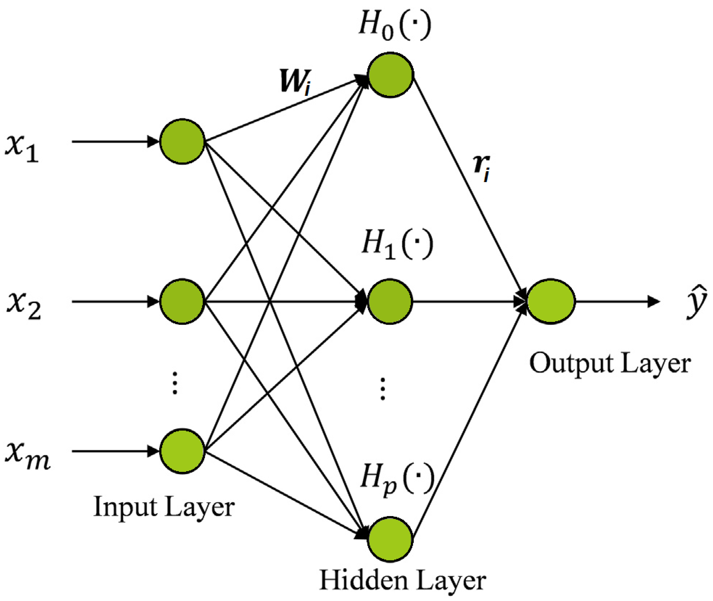
3.7. Hermite Neural Network

Here is an in-depth explanation of how the Hermite polynomial is used in the HNN construction process. Theoretically, every nonlinear function may be approximated by a neural network with an input layer, a hidden layer, and an output layer. However, conventional neural networks are notorious for their convoluted architecture and poor performance under pressure. On the other hand, the Hermite orthogonal polynomial has a straightforward recurrence relation, no range restriction on the independent variable, and minimal computing cost. Therefore, this research provides an HNN for wind speed and solar radiation forecasting by integrating best square approximation theory and neural network architecture, employing the Hermite orthogonal polynomial as the activation function of the network’s hidden layer, and employing Al-Biruni Earth Radius (BER) optimization algorithm to optimize the weights of the HNN. Figure 4 depicts the internal organization of HNN. In this figure, the structure of the HNN is $i-q-1$. The weight matrix the hidden layer receives from the input layer is denoted by $W=[W_1,W_2,\cdots ,W_q]$. For the neurons of $i=1,2,\cdots ,q$, the weight vector is denoted by $W_i={[W_1,W_2,\cdots ,W_q]}^T$. In addition, the activation function of the hidden layer is denoted by $H(.)=[H_0(.),H_1(.),\cdots ,H_p(.)]$. On the other hand, the weight vector between the output layer and the hidden layer is denoted by $r={[r_1,r_2,\cdots ,r_q]}^T$ and $q=p+1$. The bias vector of the neurons is set as 0. Therefore, hidden layer input is calculated as:

$$ne{t}_i=X_m^T{W}_i$$

(10)

Consequently, the neurons of the hidden layer has output expressed as:

$$o_i=H_{i-1}\left(ne{t}_i\right)$$

(11)

The neuron of the output layer is measured as follows:

$$\widehat{y}={[o_1,o_2,\cdots ,o_q]}^T$$

(12)

The loss function for the HNN training is the sum of the squared deviations between the actual and target values. This loss function is calculated as $L={\sum }_{i=1}^n{({\widehat{y}}_i-y_i)}^2$, where the predicted valued is denoted by ${\widehat{y}}_i$ with corresponding target values denoted by $y_i$. As a result, the optimization process may be used to find the optimal values for W and r, two of the network’s parameters, by minimizing the loss function L. Training impact is very sensitive to the choice of initial parameters, which is a problem for most conventional neural networks because gradient descent is used to maximize the networks’ weights. Even more so, its convergence rate is modest, and it’s easy for premature phenomena to emerge. The results of the experiments demonstrate that the accuracy criteria may be met by the three hidden layer nodes of HNN. On the other hand, the accuracy of predictions will not improve significantly even if the number of nodes is greatly increased and may even become overfit. With additional variables to account for, the network’s architecture will get more intricate, making parameter optimization more challenging and lengthening the time needed to model the system. Therefore, HNN has been configured with a single hidden layer and four hidden-layer nodes.

The HNN doesn’t have the problem where it’s hard to determine the number of hidden layers and neurons, as the network’s topology is straightforward, and there aren’t a lot of variables to optimize. An intense search capacity, easy operation, and rapid convergence speed are three theoretical features of the proposed optimization algorithm, which is an improved version of the Al-Biruni Earth Radius optimization algorithm. The details of the proposed optimization algorithm are presented and discussed in the next section.

3.8. Al-Biruni Earth Radius (BER) Algorithm

By dividing individuals in the search space into two groups dedicated to exploration and exploitation, the Al-Biruni Earth Radius (BER) can improve search efficiency. To maintain a reasonable equilibrium between exploitative and inquisitive pursuits, agents engage in a dynamic process of shifting the make-up of subgroups of agents. The exploration percentage is 70% of the individuals, whereas the exploitation percentage is 30%. The number of agents in both the exploration and exploitation groups has been raised to improve their global average fitness. The exploration team uses mathematical methods to look for promising new territory nearby. This is achieved by iteratively exploring all of the alternatives until one is found that possesses an optimal level of fitness source [71].

Optimization algorithms attempt to find the optimal answer within specified limits. By employing BER, we may think of each person in the population as a $\mathbf{S}$ vector. The search space is the size $S_d$, and the optimization parameter or features d is represented by the vector $\mathbf{S}=S_1,S_2,\cdots ,S_d\in R$. The fitness function F has been suggested to measure an individual’s success up to a given threshold. In these optimization stages, populations are probed to discover the value of $\mathbf{S}*$ that maximizes fitness. A random sample of the population is chosen as the first step (solutions). It is necessary to provide the fitness function, the population size, the dimension, and the minimum and maximum acceptable solution sizes before BER can optimize.

3.8.1. Exploration Operation

Exploration, as described in further depth below, is the process that finds intriguing portions of the search space and keeps the search moving ahead past the local optimum. Using this strategy, the group’s lone explorer will look for potentially fruitful new locations to explore in the immediate area around their current location, bringing them closer to the perfect answer. In addition to finding the best solution, exploration must evaluate its effectiveness. To achieve this goal, one needs to investigate the wide variety of local possibilities and pick the best for one’s health. This is achieved by the use of the following equations in BER’s studies:

$$\mathbf{S}(t+1)=\mathbf{S}\left(t\right)+\mathbf{D}(2{\mathbf{r}}_2-1),\mathbf{D}={\mathbf{r}}_1(\mathbf{S}\left(t\right)-1)$$

(13)

where $\mathbf{S}\left(t\right)$ is the solution vector at iteration t and $\mathbf{D}$ is the diameter of the circle inside which the search agent will look for interesting regions. The range of x is from 0 to 180, and the value of h is a scalar picked randomly between $[0,2]$. As instances of coefficient vectors, ${\mathbf{r}}_1$ and ${\mathbf{r}}_2$ may be found by solving the equation $\mathbf{r}=h\frac{cos\left(x\right)}{1-cos\left(x\right)}$.

3.8.2. Exploitation Operation

The team responsible for seizing chances must work to enhance the approaches that are already in place. Each cycle’s end finds the BER rewarding those who have worked hardest to reach the most significant fitness levels. Here we will discuss the two distinct methods used by the BER to achieve its exploitation goal. We can get closer to that solution if we use the following equation to guide our steps toward the best answer.

$$\mathbf{S}(t+1)={\mathbf{r}}^2(\mathbf{S}\left(t\right)+\mathbf{D}),\mathbf{D}={\mathbf{r}}_3(\mathbf{L}\left(t\right)-\mathbf{S}\left(t\right))$$

(14)

The BER uses the equation presented below to carry out the abovementioned procedure. where $\mathbf{S}\left(t\right)$ is the solution vector at iteration t, $\mathbf{L}\left(t\right)$ is the best solution vector and $\mathbf{D}$ is the distance vector, and ${\mathbf{r}}_3$ is a random vector constructed using the formula $\mathbf{r}=h\frac{cos\left(x\right)}{1-cos\left(x\right)}$ that governs the movement steps towards exploring the space around the best answer: this is the most intriguing of the possible solutions (leader). This motivates some to look for solutions close to the ideal by exploring alternatives.

$${\mathbf{S}}^{\prime }(t+1)=\mathbf{r}({\mathbf{S}}^{*}\left(t\right)+\mathbf{k}),\mathbf{k}=1+\frac{2\times t^2}{Ma{x}_{iter}^2}$$

(15)

with the optimal solution is denoted by ${\mathbf{S}}^{*}\left(t\right)$. You may choose the optimal ${\mathbf{S}}^{*}$ implementation by contrasting $\mathbf{S}(t+1)$ with ${\mathbf{S}}^{\prime }(t+1)$. If there has been no change in best fitness during the preceding two iterations, the solution will be updated using the following equation.

$$\mathbf{S}(t+1)=\mathbf{k}\ast z^2-h\frac{cos\left(x\right)}{1-cos\left(x\right)}$$

(16)

where z is a random number in the range $[0,1]$.

3.9. Genetic Algorithm (GA)

The standard GA is composed of two main steps namely, crossover and mutation. The mutation step creates a new solution with features distinct from those of the parent solutions. The mutation in nature results in the appearance of a trait previously unknown in the offspring. This ensures that the algorithm will not converge to a single optimal solution and that a wide variety of solutions will be generated [72,73]. In this work, we utilized the mutation concept to improve the exploration of the search space throughout the operation of the BER algorithm. This process is realized by mutating the positions of solutions generating by the BER algorithm at a random rate. This mutation allows exploring additional areas in the search space with potential optimal solutions, which might not be explored using the standard BER algorithm. Consequently, optimal solutions can efficiently be found using the proposed hybrid algorithm which is presented in the next section.

4. The Proposed Methodology

The proposed methodology is depicted in Figure 5. In this figure, the proposed methodology is based on two layers of forecasting. The first layer comprises a base learner set (machine learning regression models). The second layer is composed of an optimized machine-learning model called Meta-learner. The proposed modified BER model is the optimization algorithm employed in optimizing the regression model, denoted by the GABER optimization algorithm.

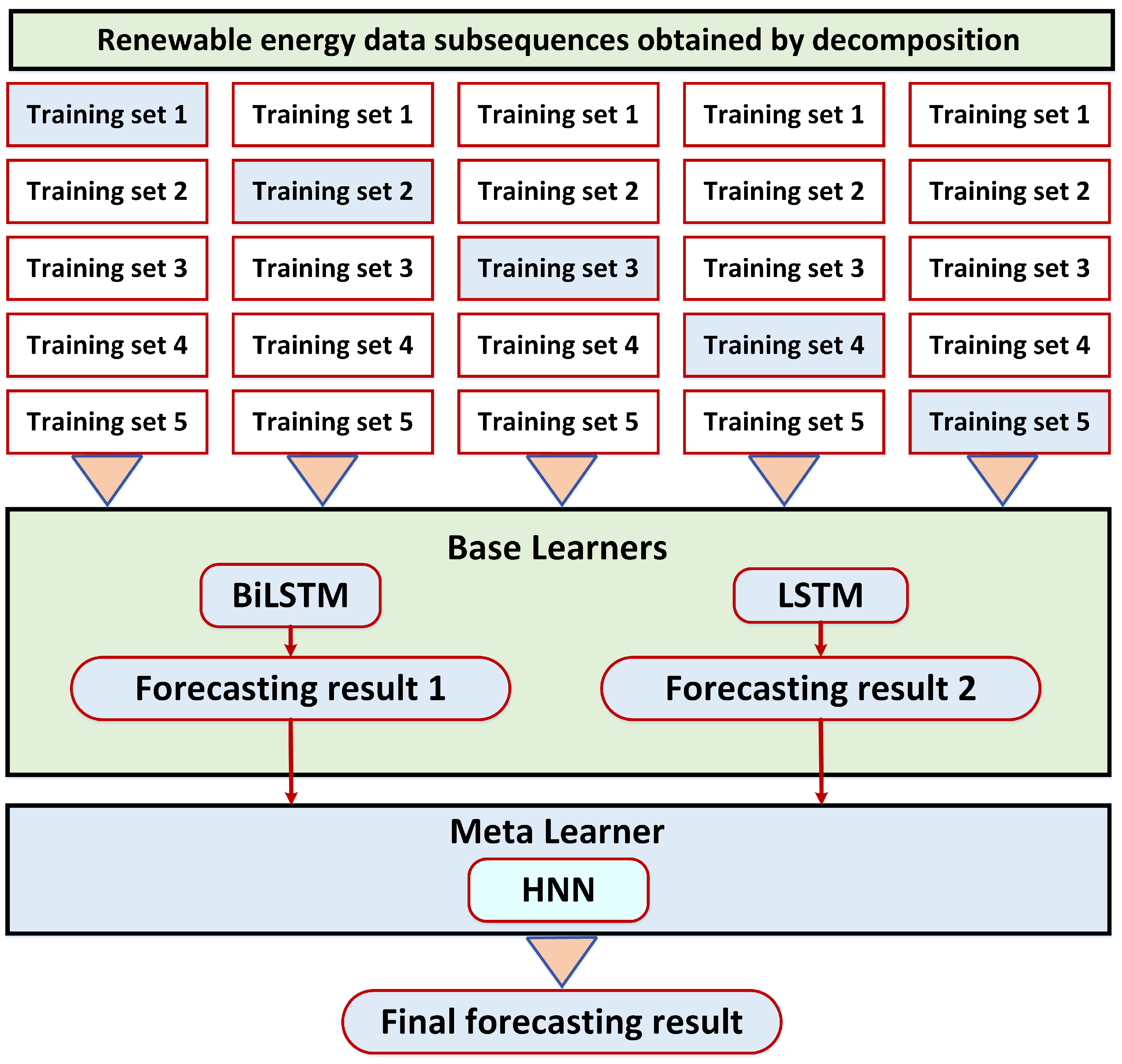
4.1. Stacking Ensemble Model

There are many different kinds of ensemble learning algorithms, and one of them is the stacking ensemble model [70]. While bagging and boosting algorithms combine identical models, the stacking ensemble model uses a variety of base learners fused in a specific way to get superior performance. As shown in Figure 5, the stacking ensemble model is a predictive model that uses a learning mechanism. We begin by creating several sub-datasets from the original dataset with nearly the same sample size. To train each base learner, the sub-datasets are input into a first-layer forecasting model, generating each learner’s forecast. The final forecasting results are achieved by combining the base learners’ outputs into a new dataset, which is then fed into the second-layer meta-learner for training. The first-layer forecasting model of the stacking ensemble model uses the k-fold cross-validation training technique to reduce the likelihood of the over-fitting phenomena occurring during the training phase. Here’s how the training itself goes down: Dataset S is randomly split into K sub-datasets $S_1$, $S_2$, etc., where n is the total number of sub-datasets. Using learner 1 as an example, we first verify each subset $S_i\{i=1;2;\cdots ,K\}$ independently, then use $K-1$ sub-dataset as a training set to acquire K forecasting outcomes, and then aggregate these K sets of results into set $D_1$ with the same length as S. The same operation is performed on the dataset for the other base learners, and the results are combined. The predicting performance of individual primary learners and the combined impact of several essential learners must be considered to create the optimal stacking ensemble model. A good base learner’s forecasting ability helps boost the total forecasting effect. The first layer of the proposed stacking ensemble model uses LSTM and BiLSTM as its foundation learners. To generalize and rectify the bias of multiple base learners for the training set, the HNN model with optimization ability is used in the second layer of the stacking model.

4.2. The Proposed Forecasting Model

Wind speed and solar radiation data are decomposed after preprocessing to reduce forecasting errors. The flow chart of the proposed forecasting model based on the proposed GABER optimization algorithm is shown in Figure 6. As shown in the figure, the steps of the flowchart are listed in the following:

• The dataset is preprocessed to avoid outliers and adjust the scale of the samples in all recordings.
• The dataset is divided into training and test sets with 5-fold cross-validation.
• The GABER-HNN model was used for training and forecasting based on the following steps:

  –

  The GABER and HNN parameters are initialized.

  –

  The fitness value is computed, and the results are shown. Within the iteration range, the parameters of the HNN are optimized, with the fitness value being the mean square error gained from training the HNN network and being updated.

  –

  The HNN is trained based on the optimal parameter combination.

• The optimized HNN is used to forecast the testing samples, and each sample’s result is saved for analysis.
• A statistical analysis is performed to measure the effectiveness and superiority of the proposed approach.

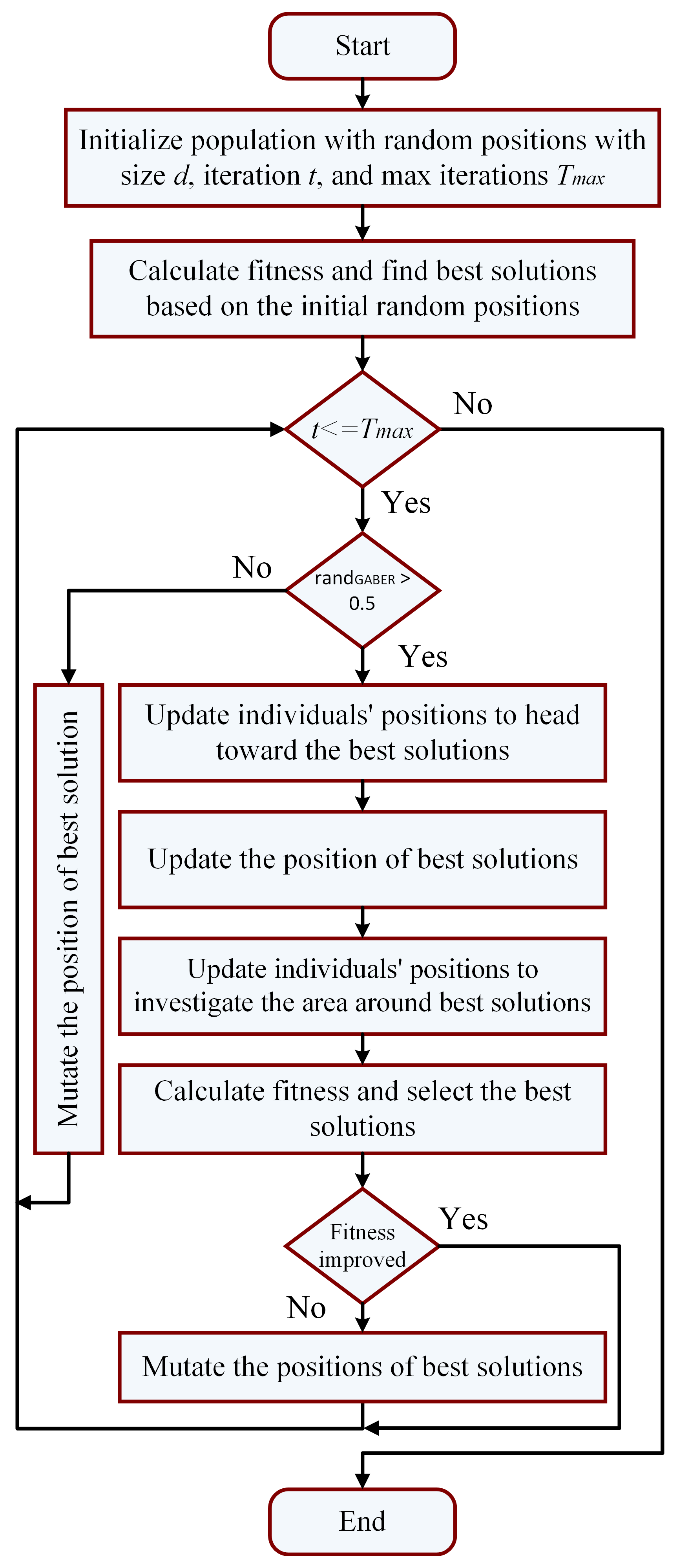
4.3. The Proposed Optimization Algorithm

The proposed Genetic Algorithm AL-Biruni Earth Radius (GABER) algorithm is described in details in Algorithm 1 and the corresponding flowchart is depicted in Figure 7. The GABER algorithm improves upon the BER and GA in terms of producing the best possible solution while avoiding their respective disadvantages. To begin, we use the notation ${\mathbf{S}}_i(i=1,2,\cdots ,d)$ to determine the initial locations of algorithm agents. It also specifies the maximum number of execution iterations, represented by $T_{max}$, and the parameters for the BER and GA algorithms. The term $ran{d}_{GABER}$ is used to describe a value that may take any value between 0 and 1 with no predictable patterns. If $ran{d}_{GABER}>0.5$, the GABER algorithm will consult the BER equations to determine how the agents’ placements should be modified. To update the agents’ locations, the GABER algorithm will employ the GA equations if $ran{d}_{GABER}\le 0.5$.

Algorithm 1: The proposed GABER algorithm

1: Initialize GABER population ${\mathbf{S}}_i(i=1,2,\cdots ,d)$ with size d, iterations $T_{max}$, fitness function $F_n$, $t=1$, GABER parameters 2: Calculate fitness function $F_n$ for each ${\mathbf{S}}_i$ 3: Find best solution as ${\mathbf{S}}^{*}$ 4: while$t\le T_{max}$do 5:    if (${rand}_{GABER}>0.5$) then 6:      for ($i=1:i<n_1+1$) do 7:         Update ${\mathbf{r}}_1=h_1\frac{cos\left(x\right)}{1-cos\left(x\right)}$, ${\mathbf{r}}_2=h_2\frac{cos\left(x\right)}{1-cos\left(x\right)}$ 8:         Calculate $\mathbf{D}={\mathbf{r}}_1(\mathbf{S}\left(t\right)-1)$ 9:         Update positions to head towards the best solution using:         $\mathbf{S}(t+1)=\mathbf{S}\left(t\right)+\mathbf{D}(2{\mathbf{r}}_2-1)$ 10:      end for 11:      for ($i=1:i<n_2+1$) do 12:         Update $\mathbf{r}=h\frac{cos\left(x\right)}{1-cos\left(x\right)}$, ${\mathbf{r}}_3=h_3\frac{cos\left(x\right)}{1-cos\left(x\right)}$ 13:         Calculate $\mathbf{D}={\mathbf{r}}_3(\mathbf{L}\left(t\right)-\mathbf{S}\left(t\right))$ 14:         Update the position of best solution using:         $\mathbf{S}(t+1)={\mathbf{r}}^2(\mathbf{S}\left(t\right)+\mathbf{D})$ 15:         Calculate $\mathbf{k}=1+\frac{2\times t^2}{Ma{x}_{iter}^2}$ 16:         Update positions to investigate area around best solution using:         ${\mathbf{S}}^{\prime }(t+1)=\mathbf{r}({\mathbf{S}}^{*}\left(t\right)+\mathbf{k})$ 17:         Compare $\mathbf{S}(t+1)$ and ${\mathbf{S}}^{\prime }(t+1)$ to select best solution ${\mathbf{S}}^{*}$ 18:         if best fitness is not changed for last two iterations then 19:           Mutate solution as $\mathbf{S}(t+1)=\mathbf{k}\ast z^2-h\frac{cos\left(x\right)}{1-cos\left(x\right)}$ 20:         end if 21:      end for 22:    else 23:      Mutate positions of the solutions using:      $\mathbf{S}(t+1)=\mathbf{k}\ast z^2-h\frac{cos\left(x\right)}{1-cos\left(x\right)}+2\left[\left({\mathbf{S}}^{\prime }(t+1)-\mathbf{S}\left(t\right)\right)-\left(1-\frac{{\mathbf{S}}^{\prime }(t+1)+\mathbf{S}\left(t\right)}{{\mathbf{S}}^{\prime }\left(t\right)}\right)\right]$ 24:    end if 25:    Update the fitness function $F_n$ for each ${\mathbf{S}}_i$ 26:    Find best solution as ${\mathbf{S}}^{*}$ 27:    Update GABER parameters, $t=t+1$ 28: end while 29: Return${\mathbf{S}}^{*}$

4.4. GABER-Based Feature Selection

In selecting the best set of features for improving the classification accuracy, the continuous output of GABER is converted into binary (0 or 1) using the following sigmoid function. The binary version of the proposed GABER algorithm is denoted by bGABER.

$$\begin{array}{cc}\hfill & P_b^{(t+1)}=\left\{\begin{array}{cc}1\hfill & \mathrm{if}Sigmoid\left(P_{Best}\right)\ge 0.5\hfill \\ 0\hfill & otherwise\hfill \end{array}\right.,\hfill \\ \hfill & Sigmoid\left(P_{Best}\right)={\displaystyle \frac{1}{1+e^{-10(P_{Best}-0.5)}}}\hfill \end{array}$$

(17)

where $P_{Best}$ refers to the best position, and t is the iteration number.

The fitness function is used to measure the quality of the solutions resulting from the optimization algorithm. The formulation of the fitness function is represented by the following equation.

$$Fitness=v_{1}Error+v_2\frac{\left|S\right|}{\left|T\right|}$$

(18)

where $Error$ represents the classification error, $\left|S\right|$ denotes the number of selected features features, and $\left|T\right|$ refers to the number of features. The factors $v_1$ and $v_2$ are in the range of $[0,1]$, where $v_1=1-v_2$.

5. Experimental Results

In this section, the proposed GABER optimization algorithm and stacking ensemble model are tested with extensive experiments to prove the effectiveness and superiority of the proposed approach. The experiments are executed on Windows 10 and Python 3.9 with an Intel(R) Core(TM) i5 CPU at 3.00 GHz (manufacturer: Intel Corporation, California, United States). The experiments were carried out in two separate case studies. In the first case study, we compare the performance of the GABER method to that of baseline models on the wind speed dataset. The proposed method is evaluated in terms of the solar radiation dataset in the second case study. The settings for the GABER algorithm configuration are presented in

Table 1. Configuration parameters of GABER algorithm.

Parameter	Values
# Agents	10
# Iterations	80
# Repetitions	20
$\eta$	$\in [0,1]$
Mutation probability	0.5
Exploration percentage	70
k (decreases from 2 to 0)	1

and the settings of the other optimization algorithms included in the conducted experiments are shown in

Table 2. Configuration parameters of the competing optimization algorithms.

Algorithm	Parameter	Values
GA	Cross over	0.9
	Mutation ratio	0.1
	Selection mechanism	Roulette wheel
	Iterations	80
	Agents	10
PSO	Acceleration constants	[2, 2]
	Inertia $W_{max}$, $W_{min}$	[0.6, 0.9]
	Particles	10
	Iterations	80
GWO	a	2 to 0
	Iterations	80
	Wolves	10
WOA	r	[0, 1]
	Iterations	80
	Whales	10
	a	2 to 0

.

5.1. Evaluation Metrics

The achieved results are assessed in terms of the criteria presented in

Table 3. Feature selection results evaluation criteria.

Metric	Formula
Best Fitness	$mi{n}_{i=1}^M{S}_i^{*}$
Worst Fitness	$ma{x}_{i=1}^M{S}_i^{*}$
Average Error	$\frac{1}{M}{\sum }_{j=1}^M\frac{1}{N}{\sum }_{i=1}^{N}mse(\widehat{V_i}-V_i)$
Average Fitness	$\frac{1}{M}{\sum }_{i=1}^M{S}_i^{*}$
Average fitness size	$\frac{1}{M}{\sum }_{i=1}^{M}size\left(S_i^{*}\right)$
Standard deviation	$\sqrt{\frac{1}{M-1}{\sum }_{i=1}^M{\left(S_i^{*}-Mean\right)}^2}$

. The criteria listed in this table are used to evaluate the performance of the proposed feature selection method [74,75,76,77,78]. In addition, in this table, the number of runs of the proposed and other competing optimizers is indicated as M. The best solution at the run number j is denoted by $S_j^{*}$, $size\left(S_j^{*}\right)$ refers to the size of the best solution vector. N denoted the number of points in the test set. $\widehat{V_n}$ and $V_n$ refer to the predicted and actual values, respectively.

On the other hand, additional metrics are used to measure the performance of the regression models employed to predict wind speed and solar radiation. These metrics include root mean error (RMSE), mean absolute error (MAE), mean bias error (MBE), Pearson’s correlation coefficient (r), coefficient of determination ($R^2$), Relative RMSE (RRMSE), Nash Sutcliffe Efficiency (NSE), determine agreement (WI), where N is the number of observations in the dataset; ($\widehat{V_n}$) and ($V_n$) are the $n^{th}$ estimated and observed bandwidth, and ($\overline{\widehat{V_n}}$) and ($V_n$) are the arithmetic means of the estimated and observed values. These metrics are evaluated using the equations presented in

Table 4. Prediction results evaluation criteria.

Metric	Formula
RMSE	$\sqrt{\frac{1}{N}{\sum }_{n=1}^N{(\widehat{V_n}-V_n)}^2}$
RRMSE	$\frac{RMSE}{{\sum }_{n=1}^N\widehat{V_n}}\times 100$
MAE	$\frac{1}{N}{\sum }_{n=1}^N|\widehat{V_n}-V_n|$
MBE	$\frac{1}{N}{\sum }_{n=1}^N(\widehat{V_n}-V_n)$
NSE	$1-\frac{{\sum }_{n=1}^N{(V_n-\widehat{V_n})}^2}{{\sum }_{n=1}^N{(V_n-\overline{\widehat{V_n}})}^2}$
WI	$1-\frac{{\sum }_{n=1}^N|\widehat{V_n}-V_n|}{{\sum }_{n=1}^N|V_n-\overline{V_n}|+|\widehat{V_n}-\overline{\widehat{V_n}}|}$
$R^2$	$1-\frac{{\sum }_{n=1}^N{(V_n-\widehat{V_n})}^2}{{\sum }_{n=1}^N{\left({\sum }_{n=1}^N{V}_n)-V_n\right)}^2}$
r	$\frac{{\sum }_{n=1}^N(\widehat{V_n}-\overline{\widehat{V_n}})(V_n-\overline{V_n})}{\sqrt{\left({\sum }_{n=1}^N{(\widehat{V_n}-\overline{\widehat{V_n}})}^2\right)\left({\sum }_{n=1}^N{(V_n-\overline{V_n})}^2\right)}}$

.

5.2. Wind Speed Prediction Results

The evaluation of the proposed approach for predicting wind speed is presented in this section. The evaluation is performed using the proposed feature selection algorithm and the proposed GABER-based optimized stacked ensemble model. The coming section presents the recorded results with a description.

5.2.1. Feature Selection Results

The proposed feature selection method is evaluated using the wind speed dataset. The measured results are presented in

Table 5. Evaluation of the proposed feature selection method using the wind speed dataset.

	bGABER	bBER	bGA	bPSO	bGWO	bWOA
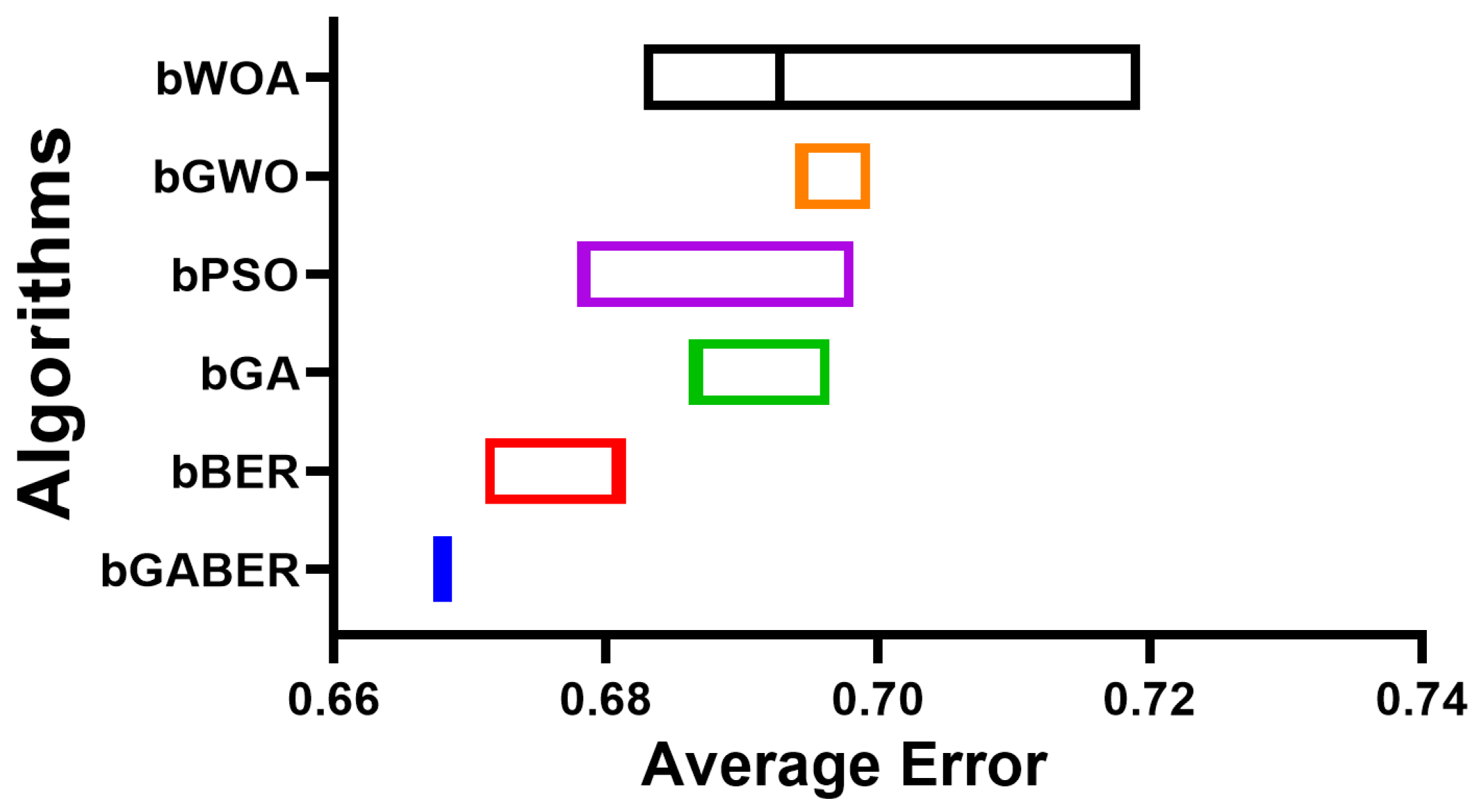
Average Error	0.6680	0.6811	0.6865	0.6782	0.6942	0.6928
Average Select Size	0.8683	0.9617	0.9700	0.9700	0.9784	0.97003
Average Fitness	0.8043	0.8523	0.8575	0.8494	0.8652	0.86379
Best Fitness	0.7696	0.7888	0.7792	0.7792	0.7984	0.7984
Worst Fitness	0.9114	0.8946	0.9234	0.9234	0.9618	1.06756
Std Fitness	0.3233	0.3261	0.3373	0.3350	0.3377	0.3613
Processing Time (S)	13.513	14.336	14.896	14.456	14.82	15.132

. In this table, it can be noted that the proposed bGABER method achieved the best results when considering all the evaluation criteria of feature selection presented in the previous section.

The statistical difference and significance of the proposed feature selection are tested using two statistical tests: the one-way analysis of variance (ANOVA) test and the Wilcoxon signed-rank test. These tests are based on two hypotheses denoted by H0 and H1. The results of these tests are presented in

Table 6. ANOVA of the proposed feature selection method based on the wind speed dataset.

	SS	DF	MS	F (DFn, DFd)	p Value
Treatment	0.005468	5	0.001094	F (5, 54) = 41.67	p < 0.0001
Residual	0.001417	54	0.00002624
Total	0.006885	59

and

Table 7. Wilcoxon of the proposed feature selection method based on the wind speed dataset.

	bGABER	bBER	bGA	bPSO	bGWO	bWOA
Theoretical median	0	0	0	0	0	0
Actual median	0.668	0.681	0.686	0.678	0.694	0.692
Number of values	10	10	10	10	10	10
Wilcoxon Test
Sum of signed ranks	55	55	55	55	55	55
Sum of +ve ranks	55	55	55	55	55	55
Sum of −ve ranks	0	0	0	0	0	0
p value (two tailed)	0.002	0.002	0.002	0.002	0.002	0.002
Exact or estimate?	Exact	Exact	Exact	Exact	Exact	Exact
Significant?	Yes	Yes	Yes	Yes	Yes	Yes
Discrepancy	0.668	0.6811	0.6865	0.6782	0.6942	0.6928

, respectively. The results presented in these tables indicate the statistical significance of the proposed approach in selecting the best set of features that can improve the wind speed prediction results.

In addition, the plot shown in Figure 8 depicts the average error of the results achieved by the proposed feature selection methods compared to the other five feature selection methods. In this plot, the proposed feature selection method achieved the minimum average error value, which reflects its effectiveness and superiority.

On the other hand, the plots shown in Figure 9 illustrate the performance of the proposed feature selection method when tested on the wind speed dataset. In these plots, the tiny residual error with reasonable fitting between the predicted and actual residuals can be noted. In addition, the heatmap shows a significant impact of the proposed method compared to the other feature selection methods.

5.2.2. Prediction Results

The prediction results are evaluated in

Table 8. Evaluation of the prediction results achieved by the proposed optimized stacked ensemble model applied to the wind speed dataset.

	RMSE	MAE	MBE	r	${\mathit{R}}^2$	RRMSE	NSE	WI
LSTM	0.0095	0.0069	−0.0006	0.9605	0.9226	19.1545	0.9218	0.8868
BILSTM	0.0031	0.0020	−0.0002	0.9952	0.9904	8.3202	0.9903	0.9630
Non-Optimized HNN Ensemble	0.0011	0.0007	−0.0001	0.9994	0.9989	3.3862	0.9989	0.9885
Proposed Optimized HNN Ensemble	0.0003	0.0003	0.0000	0.9997	0.9995	2.2035	0.9995	0.9922

. This table presents the prediction results achieved by the proposed optimized HNN stacked ensemble compared to those performed by LSTM, BILSTM, and non-optimized HNN ensemble. The results presented in this table prove the effectiveness and superiority of the proposed approach. The proposed approach achieves the minimum RMSE, MAE, MBE, and RRMSE values. The proposed approach also achieves the maximum r, $R^2$, NSE, and WI values. These results emphasize the effectiveness of the proposed approach. In addition, a statistical analysis is performed on the prediction results and presented in

Table 9. Statistical analysis of the prediction results achieved by the proposed optimized stacked ensemble model applied to the wind speed dataset.

	GABER	BER	GA	PSO	GWO	WOA
Number of values	10	10	10	10	10	10
Range	0.00002	0.00014	0.0001	0.0002	0.000124	0.0001
Minimum	0.000333	0.000457	0.00052	0.000599	0.000785	0.000871
Mean	0.000343	0.000551	0.0005924	0.000699	0.0008039	0.0009126
Maximum	0.000353	0.000597	0.00062	0.000799	0.000909	0.000971
Median	0.000343	0.000557	0.000598	0.000699	0.000785	0.000912
75% Percentile	0.000343	0.000557	0.000598	0.000699	0.0008013	0.000922
25% Percentile	0.000343	0.000557	0.000598	0.000699	0.000785	0.0008885
Std. Deviation	0.000004714	0.00003534	0.00002636	0.00004714	0.0000422	0.00003011
Std. Error of Mean	0.000001491	0.00001118	0.000008336	0.00001491	0.00001335	0.000009522
Sum	0.00343	0.00551	0.005924	0.00699	0.008039	0.009126

. In this table, the statistical analysis results are compared to the other five optimization algorithms. The analysis results and comparison show the superiority of the proposed optimized stacked ensemble.

Moreover, another set of experiments is conducted to study the statistical difference and significance of the proposed optimized stacked ensemble. This set includes the ANOVA and Wilcoxon signed-rank tests. The results of these tests are presented in

Table 10. ANOVA test applied to the prediction results achieved by the proposed optimized ensemble model applied to the wind speed dataset.

	SS	DF	MS	F (DFn, DFd)	p-Value
Treatment	0.000002024	5	$4.048\times {10}^{-7}$	F (5, 54) = 353.3	p < 0.0001
Residual	$6.188\times {10}^{-8}$	54	$1.146\times {10}^{-9}$
Total	0.000002086	59

and

Table 11. Wilcoxon test applied the prediction results achieved by the proposed optimized ensemble model applied to the wind speed dataset.

	GABER	BER	GA	PSO	GWO	WOA
Theoretical median	0	0	0	0	0	0
Actual median	0.000343	0.000557	0.000598	0.000699	0.000785	0.000912
Number of values	10	10	10	10	10	10
Sum of signed ranks	55	55	55	55	55	55
Sum of +ve ranks	55	55	55	55	55	55
Sum of −ve ranks	0	0	0	0	0	0
p-value	0.002	0.002	0.002	0.002	0.002	0.002
Exact or estimate?	Exact	Exact	Exact	Exact	Exact	Exact
Significant?	Yes	Yes	Yes	Yes	Yes	Yes
Discrepancy	0.000343	0.000557	0.000598	0.000699	0.000785	0.000912

, respectively. From Table 10, the p-value is less than $0.005$, indicating a statistical difference between the proposed approach and other methods included in the conducted experiments. Similarly, the p-value in the results recorded in Table 11 confirms the statistical difference and significance of the proposed approach.

On the other hand, the wind speed prediction results are visually analyzed as depicted in the plots shown in Figure 10. These plots show a promising performance of the proposed approach in predicting wind speed. These plots include residual, homoscedasticity, quartile-quartile (QQ), and heatmap. The residual and homoscedasticity show a minimal error in predicting the wind speed, whereas QQ and heatmap plots show a robust prediction.

To clearly show the robustness of the proposed optimized stacked ensemble, Figure 11 shows the RMSE values achieved by the proposed method compared to the other five methods. The proposed method achieves the minimum RMSE value, reflecting its robustness.

5.3. Solar Radiation Prediction Results

The evaluation of the proposed approach for predicting solar radiation is presented in this section. The evaluation is performed using the proposed feature selection algorithm and the proposed GABER-based optimized stacked ensemble model. The coming section presents the recorded results with a description.

5.3.1. Feature Selection Results

The solar radiation dataset is used to analyze the proposed feature selection approach.

Table 12. Evaluation of the proposed feature selection method when applied to the solar radiation dataset.

	bGABER	bBER	bGA	bPSO	bGWO	bWOA
Average Error	0.3904	0.4035	0.4088	0.4006	0.4166	0.4152
Average Select Size	0.5907	0.6841	0.6924	0.6924	0.7008	0.6924
Average Fitness	0.5267	0.5746	0.5799	0.5718	0.5876	0.5862
Best Fitness	0.4920	0.5112	0.5016	0.5016	0.5208	0.5208
Worst Fitness	0.6338	0.6169	0.6458	0.6458	0.6842	0.7899
Std Fitness	0.0457	0.0485	0.0597	0.0574	0.0600	0.0837
Processing Time (s)	7.783	8.606	9.166	8.726	9.09	9.402

displays the measured data. According to this table, the proposed bGABER algorithm outperformed the other methods in terms of all the assessment criteria of feature selection.

The ANOVA and Wilcoxon tests are used to examine the statistical differences and significance of the proposed feature selection when applied to solar radiation prediction. The H0 and H1 hypotheses form the basis for these examinations.

Table 13. ANOVA test of the results achieved by the proposed feature selection method when applied to the solar radiation dataset.

	SS	DF	MS	F (DFn, DFd)	p-Value
Treatment	0.007312	5	0.001462	F (5, 54) = 19.40	p < 0.0001
Residual	0.00407	54	0.00007538
Total	0.01138	59

and

Table 14. Wilcoxon test of the results achieved by the proposed feature selection method when applied to the solar radiation dataset.

	bGABER	bBER	bGA	bPSO	bGWO	bWOA
Theoretical median	0	0	0	0	0	0
Actual median	0.3904	0.4035	0.4088	0.4006	0.4166	0.4152
Number of values	10	10	10	10	10	10
Wilcoxon Signed Rank Test
Sum of signed ranks (W)	55	55	55	55	55	55
Sum of +ve ranks	55	55	55	55	55	55
Sum of −ve ranks	0	0	0	0	0	0
p-value (two tailed)	0.002	0.002	0.002	0.002	0.002	0.002
Exact or estimate?	Exact	Exact	Exact	Exact	Exact	Exact
Significant?	Yes	Yes	Yes	Yes	Yes	Yes
Discrepancy	0.3904	0.4035	0.4088	0.4006	0.4166	0.4152

display the results of these analyses, respectively. The table shows that the suggested method is statistically significant in choosing the appropriate collection of features to enhance solar radiation prediction outcomes.

Figure 12 shows the results of testing the proposed feature selection approach on the solar radiation dataset. The acceptable match between the predicted and actual residuals is shown in these figures, with little residual error clearly shown in the figure. Compared to alternative feature selection methods, the heatmap also demonstrates the suggested approach’s substantial influence on the feature selection quality when applied to the solar radiation dataset.

The average error of the results produced by the proposed feature selection method in contrast to the other five feature selection methods is also depicted graphically in Figure 13. This graph demonstrates the usefulness and superiority of the suggested feature selection approach by displaying the least average error value.

5.3.2. Prediction Results

Table 15. Evaluation of the prediction results based on the solar radiation dataset.

	RMSE	MAE	MBE	r	${\mathit{R}}^2$	RRMSE	NSE	WI
LSTM	0.00423	0.00307	−0.00026	0.96085	0.92293	15.46608	0.92217	0.88721
BILSTM	0.00138	0.00090	−0.00008	0.99552	0.99073	4.95515	0.99068	0.96332
Non-Optimized HNN Ensemble	0.00049	0.00031	−0.00003	0.99980	0.99926	3.23935	0.99925	0.98883
Proposed Optimized HNN Ensemble	0.00015	0.00011	0.00001	0.99990	0.99986	0.91144	0.99985	0.99260

displays the outcomes of examining the forecasts. The table below shows how the proposed optimized HNN stacked ensemble performed in prediction compared to the LSTM, BILSTM, and non-optimized HNN ensemble. It is clear from this table that the proposed method is superior and efficient. The suggested method minimizes the RMSE, MAE, MBE, and RRMSE. Additionally, the suggested approach maximizes r, $R^2$, NSE, and WI. The outcomes demonstrated the efficacy of the proposed method.

Table 16. Statistical analysis of the prediction results achieved by the proposed optimized ensemble model when applied to the solar radiation dataset.

	GABER	BER	GA	PSO	GWO	WOA
Number of values	10	10	10	10	10	10
Range	0	0.0001	0.00012	0.0001	0.0002	0.0003
Maximum	0.000153	0.000373	0.000439	0.000512	0.000717	0.000974
Mean	0.000153	0.0003614	0.000411	0.0004941	0.000617	0.000854
Minimum	0.000153	0.000273	0.000319	0.000412	0.000517	0.000674
Median	0.000153	0.000373	0.000419	0.000512	0.000617	0.000874
75% Percentile	0.000153	0.000373	0.000419	0.000512	0.000617	0.000874
25% Percentile	0.000153	0.000369	0.000419	0.0004923	0.000617	0.000849
Std. Deviation	0	0.00003146	0.00003293	0.00003806	0.00004714	0.00007888
Std. Error of Mean	0	0.00000995	0.00001041	0.00001204	0.00001491	0.00002494
Sum	0.00153	0.003614	0.00411	0.004941	0.00617	0.00854

displays the results of a statistical analysis done on the predictions. This table compares the statistical analysis’s results with five different optimization strategies. The comparison and analysis findings support the idea that the proposed optimized stacked ensemble is the best option.

The statistical variation and importance of the suggested optimized stacked ensemble are also investigated in the second series of experiments. Among the tests that are included are the ANOVA and Wilcoxon signed-rank tests.

Table 17. ANOVA test applied to the results of the proposed optimized ensemble when applied to the solar radiation dataset.

	SS	DF	MS	F (DFn, DFd)	p Value
Treatment	0.000002846	5	$5.692\times {10}^{-7}$	F (5, 54) = 285.4	p < 0.0001
Residual	$1.077\times {10}^{-7}$	54	$1.995\times {10}^{-9}$
Total	0.000002954	59

and

Table 18. Wilcoxon test applied to the results achieved by the proposed optimized ensemble when applied to the solar radiation dataset.

	GABER	BER	GA	PSO	GWO	WOA
Theoretical median	0	0	0	0	0	0
Actual median	0.000153	0.000373	0.000419	0.000512	0.000617	0.000874
Number of values	10	10	10	10	10	10
Wilcoxon Signed Rank Test
Sum of signed ranks	55	55	55	55	55	55
Sum of +ve ranks	55	55	55	55	55	55
Sum of −ve ranks	0	0	0	0	0	0
p-value (two tailed)	0.002	0.002	0.002	0.002	0.002	0.002
Exact or estimate?	Exact	Exact	Exact	Exact	Exact	Exact
Significant?	Yes	Yes	Yes	Yes	Yes	Yes
Discrepancy	0.000153	0.000373	0.000419	0.000512	0.000617	0.000874

display the findings of these statistical tests. The proposed method shows statistical significance in comparison to the other techniques used in the experiments (with p < 0.005), as shown in Table 17. The p-value also confirms the statistical difference and significance of the suggested method in the findings recorded in Table 18.

The plots shown in Figure 14 provide for visual analysis of the outcomes of the wind speed predictions. These plots demonstrate the potential of the proposed method for predicting solar radiation. The residual, homoscedasticity, QQ, and heatmap plots are also included in the figure. The QQ and heatmap plots and the residual and homoscedasticity statistics demonstrate highly accurate solar radiation forecasting.

Figure 15 demonstrates the robustness of the proposed optimized stacked ensemble by comparing the RMSE values attained by the suggested technique with those of the other five methods. With the suggested strategy, the RMSE is minimized, demonstrating its reliability.

6. Conclusions

To predict wind speed and solar energy radiation, this paper introduces a novel optimization algorithm based on a modification applied to the recently emerged BER algorithm inspired by the mutation of the genetic algorithm and is referred to as the GABER algorithm. The proposed optimization algorithm is employed to optimize a new stacked ensemble model consisting of two levels; the first is composed of two prediction models, namely LSTM and BILSTM, and the second is composed of the HNN model. The HNN model in the proposed stacked ensemble model is optimized using the proposed GABER algorithm to improve the prediction accuracy of wind speed and solar radiation. To show the superiority of the proposed approach, a set of experiments is conducted based on five other optimization methods and three other prediction models in terms of the wind speed and solar radiation datasets. Experimental results showed the superiority and effectiveness of the proposed approach in predicting both wind speed and solar radiation. This proved the generalization of the proposed method in accurately predicting renewable energy. On the other hand, statistical tests were conducted to study the statistical difference and significance of the proposed approach. The recorded results confirmed the expected findings. The potential future perspectives of the proposed approach are to evaluate it in terms of other datasets of significant scale to emphasize its generalization.

References

- Alkesaiberi, A.; Harrou, F.; Sun, Y. Efficient Wind Power Prediction Using Machine Learning Methods: A Comparative Study. Energies 2022, 15, 2327. [Google Scholar] [CrossRef]
- Hanifi, S.; Liu, X.; Lin, Z.; Lotfian, S. A Critical Review of Wind Power Forecasting Methods—Past, Present and Future. Energies 2020, 13, 3764. [Google Scholar] [CrossRef]
- Treiber, N.A.; Heinermann, J.; Kramer, O. Wind Power Prediction with Machine Learning. In Computational Sustainability; Lässig, J., Kersting, K., Morik, K., Eds.; Springer International Publishing: Cham, Switzerland, 2016; pp. 13–29. [Google Scholar] [CrossRef]
- Mao, Y.; Shaoshuai, W. A review of wind power forecasting & prediction. In Proceedings of the 2016 International Conference on Probabilistic Methods Applied to Power Systems (PMAPS), Beijing, China, 16–20 October 2016; pp. 1–7. [Google Scholar] [CrossRef]
- Ouyang, T.; Zha, X.; Qin, L.; He, Y.; Tang, Z. Prediction of wind power ramp events based on residual correction. Renew Energy 2019, 136, 781–792. [Google Scholar] [CrossRef]
- Ding, F.; Tian, Z.; Zhao, F.; Xu, H. An integrated approach for wind turbine gearbox fatigue life prediction considering instantaneously varying load conditions. Renew Energy 2018, 129, 260–270. [Google Scholar] [CrossRef]
- Han, S.; hui Qiao, Y.; Yan, J.; qian Liu, Y.; Li, L.; Wang, Z. Mid-to-long term wind and photovoltaic power generation prediction based on copula function and long short term memory network. Appl. Energy 2019, 239, 181–191. [Google Scholar] [CrossRef]
- Tascikaraoglu, A.; Uzunoglu, M. A review of combined approaches for prediction of short-term wind speed and power. Renew. Sustain. Energy Rev. 2014, 34, 243–254. [Google Scholar] [CrossRef]
- Bouyeddou, B.; Harrou, F.; Saidi, A.; Sun, Y. An Effective Wind Power Prediction using Latent Regression Models. In Proceedings of the 2021 International Conference on ICT for Smart Society (ICISS), Bandung City, Indonesia, 2–4 August 2021; pp. 1–6. [Google Scholar] [CrossRef]
- Yan, J.; Ouyang, T. Advanced wind power prediction based on data-driven error correction. Energy Convers. Manag. 2019, 180, 302–311. [Google Scholar] [CrossRef]
- Karakuş, O.; Kuruoğlu, E.E.; Altınkaya, M.A. One-day ahead wind speed/power prediction based on polynomial autoregressive model. IET Renew. Power Gener. 2017, 11, 1430–1439. [Google Scholar] [CrossRef]
- Wang, Y.; Zou, R.; Liu, F.; Zhang, L.; Liu, Q. A review of wind speed and wind power forecasting with deep neural networks. Appl. Energy 2021, 304, 117766. [Google Scholar] [CrossRef]
- Rajagopalan, S.; Santoso, S. Wind power forecasting and error analysis using the autoregressive moving average modeling. In Proceedings of the 2009 IEEE Power & Energy Society General Meeting, Calgary, AB, Canada, 26–30 July 2009; pp. 1–6, ISSN: 1932-5517. [Google Scholar] [CrossRef]
- Singh, P.K.; Singh, N.; Negi, R. Wind Power Forecasting Using Hybrid ARIMA-ANN Technique. In Advances in Intelligent Systems and Computing, Proceedings of the Ambient Communications and Computer Systems, Ajmer, India, 16–17 August 2019; Hu, Y.C., Tiwari, S., Mishra, K.K., Trivedi, M.C., Eds.; Springer: Singapore, 2019; pp. 209–220. [Google Scholar]
- Sayed, E.T.; Wilberforce, T.; Elsaid, K.; Rabaia, M.K.H.; Abdelkareem, M.A.; Chae, K.J.; Olabi, A.G. A critical review on environmental impacts of renewable energy systems and mitigation strategies: Wind, hydro, biomass and geothermal. Sci. Total. Environ. 2021, 766, 144505. [Google Scholar] [CrossRef]
- Araujo, J.M.S.d. Improvement of Coding for Solar Radiation Forecasting in Dili Timor Leste—A WRF Case Study. J. Power Energy Eng. 2021, 9, 7–20. [Google Scholar] [CrossRef]
- Ziane, A.; Necaibia, A.; Sahouane, N.; Dabou, R.; Mostefaoui, M.; Bouraiou, A.; Khelifi, S.; Rouabhia, A.; Blal, M. Photovoltaic output power performance assessment and forecasting: Impact of meteorological variables. Sol. Energy 2021, 220, 745–757. [Google Scholar] [CrossRef]
- Alawasa, K.M.; Al-Odienat, A.I. Power quality characteristics of residential grid-connected inverter ofphotovoltaic solar system. In Proceedings of the 2017 IEEE 6th International Conference on Renewable Energy Research and Applications (ICRERA), San Diego, CA, USA, 5–8 November 2017; pp. 1097–1101. [Google Scholar] [CrossRef]
- Gielen, D.; Boshell, F.; Saygin, D.; Bazilian, M.D.; Wagner, N.; Gorini, R. The role of renewable energy in the global energy transformation. Energy Strategy Rev. 2019, 24, 38–50. [Google Scholar] [CrossRef]
- Strielkowski, W.; Civín, L.; Tarkhanova, E.; Tvaronavičienė, M.; Petrenko, Y. Renewable Energy in the Sustainable Development of Electrical Power Sector: A Review. Energies 2021, 14, 8240. [Google Scholar] [CrossRef]
- Lay-Ekuakille, A.; Ciaccioli, A.; Griffo, G.; Visconti, P.; Andria, G. Effects of dust on photovoltaic measurements: A comparative study. Measurement 2018, 113, 181–188. [Google Scholar] [CrossRef]
- McGee, T.G.; Mori, K. The Management of Urbanization, Development, and Environmental Change in the Megacities of Asia in the Twenty-First Century. In Living in the Megacity: Towards Sustainable Urban Environments; Muramatsu, S., McGee, T.G., Mori, K., Eds.; Global Environmental Studies, Springer: Tokyo, Japan, 2021; pp. 17–33. [Google Scholar] [CrossRef]
- Wilson, G.A.; Bryant, R.L. Environmental Management: New Directions for the Twenty-First Century, 1st ed.; Routledge: London, UK, 2021. [Google Scholar] [CrossRef]
- Ismail, A.M.; Ramirez-Iniguez, R.; Asif, M.; Munir, A.B.; Muhammad-Sukki, F. Progress of solar photovoltaic in ASEAN countries: A review. Renew. Sustain. Energy Rev. 2015, 48, 399–412. [Google Scholar] [CrossRef]
- Al-Odienat, A.; Al-Maitah, K. A modified Active Frequency Drift Method for Islanding Detection. In Proceedings of the 2021 12th International Renewable Engineering Conference (IREC), Amman, Jordan, 14–15 April 2021; pp. 1–6. [Google Scholar] [CrossRef]
- Srivastava, R.; Tiwari, A.N.; Giri, V.K. Prediction of Electricity Generation using Solar Radiation Forecasting Data. In Proceedings of the 2020 International Conference on Electrical and Electronics Engineering (ICE3), Gorakhpur, India, 14–15 February 2020; pp. 168–172. [Google Scholar] [CrossRef]
- Alawasa, K.M.; Al-Odienat, A.I. Power Quality Investigation of Single Phase Grid-connected Inverter of Photovoltaic System. J. Eng. Technol. Sci. 2019, 51, 597–614. [Google Scholar] [CrossRef]
- Bhaskar, K.; Singh, S.N. AWNN-Assisted Wind Power Forecasting Using Feed-Forward Neural Network. IEEE Trans. Sustain. Energy 2012, 3, 306–315. [Google Scholar] [CrossRef]
- Chen, N.; Qian, Z.; Nabney, I.T.; Meng, X. Wind Power Forecasts Using Gaussian Processes and Numerical Weather Prediction. IEEE Trans. Power Syst. 2014, 29, 656–665. [Google Scholar] [CrossRef]
- Azimi, R.; Ghofrani, M.; Ghayekhloo, M. A hybrid wind power forecasting model based on data mining and wavelets analysis. Energy Convers. Manag. 2016, 127, 208–225. [Google Scholar] [CrossRef]
- Yang, L.; He, M.; Zhang, J.; Vittal, V. Support-Vector-Machine-Enhanced Markov Model for Short-Term Wind Power Forecast. IEEE Trans. Sustain. Energy 2015, 6, 791–799. [Google Scholar] [CrossRef]
- Ti, Z.; Deng, X.W.; Zhang, M. Artificial Neural Networks based wake model for power prediction of wind farm. Renew. Energy 2021, 172, 618–631. [Google Scholar] [CrossRef]
- Saroha, S.; Aggarwal, S.K. Wind power forecasting using wavelet transforms and neural networks with tapped delay. CSEE J. Power Energy Syst. 2018, 4, 197–209. [Google Scholar] [CrossRef]
- Dowell, J.; Pinson, P. Very-Short-Term Probabilistic Wind Power Forecasts by Sparse Vector Autoregression. IEEE Trans. Smart Grid 2016, 7, 763–770. [Google Scholar] [CrossRef]
- Wu, J.L.; Ji, T.Y.; Li, M.S.; Wu, P.Z.; Wu, Q.H. Multistep Wind Power Forecast Using Mean Trend Detector and Mathematical Morphology-Based Local Predictor. IEEE Trans. Sustain. Energy 2015, 6, 1216–1223. [Google Scholar] [CrossRef]
- Demolli, H.; Dokuz, A.S.; Ecemis, A.; Gokcek, M. Wind power forecasting based on daily wind speed data using machine learning algorithms. Energy Convers. Manag. 2019, 198, 111823. [Google Scholar] [CrossRef]
- Lekkas, D.; Price, G.D.; Jacobson, N.C. Using smartphone app use and lagged-ensemble machine learning for the prediction of work fatigue and boredom. Comput. Hum. Behav. 2022, 127, 107029. [Google Scholar] [CrossRef]
- Bi, J.W.; Han, T.Y.; Li, H. International tourism demand forecasting with machine learning models: The power of the number of lagged inputs. Tour. Econ. 2022, 28, 621–645. [Google Scholar] [CrossRef]
- Shang, H.L. Dynamic principal component regression for forecasting functional time series in a group structure. Scand. Actuar. J. 2020, 2020, 307–322. [Google Scholar] [CrossRef]
- Liu, Y.; Sun, Y.; Infield, D.; Zhao, Y.; Han, S.; Yan, J. A Hybrid Forecasting Method for Wind Power Ramp Based on Orthogonal Test and Support Vector Machine (OT-SVM). IEEE Trans. Sustain. Energy 2017, 8, 451–457. [Google Scholar] [CrossRef]
- Yuan, X.; Chen, C.; Yuan, Y.; Huang, Y.; Tan, Q. Short-term wind power prediction based on LSSVM–GSA model. Energy Convers. Manag. 2015, 101, 393–401. [Google Scholar] [CrossRef]
- Buturache, A.N.; Stancu, S. Wind Energy Prediction Using Machine Learning. Low Carbon Econ. 2021, 12, 1–21. [Google Scholar] [CrossRef]
- Liu, T.; Wei, H.; Zhang, K. Wind power prediction with missing data using Gaussian process regression and multiple imputation. Appl. Soft Comput. 2018, 71, 905–916. [Google Scholar] [CrossRef]
- Deng, Y.; Jia, H.; Li, P.; Tong, X.; Qiu, X.; Li, F. A Deep Learning Methodology Based on Bidirectional Gated Recurrent Unit for Wind Power Prediction. In Proceedings of the 2019 14th IEEE Conference on Industrial Electronics and Applications (ICIEA), Xi’an, China, 19–21 June 2019; pp. 591–595. [Google Scholar] [CrossRef]
- Xiaoyun, Q.; Xiaoning, K.; Chao, Z.; Shuai, J.; Xiuda, M. Short-term prediction of wind power based on deep Long Short-Term Memory. In Proceedings of the 2016 IEEE PES Asia–Pacific Power and Energy Engineering Conference (APPEEC), Xi’an, China, 25–28 October 2016; pp. 1148–1152. [Google Scholar] [CrossRef]
- Castangia, M.; Aliberti, A.; Bottaccioli, L.; Macii, E.; Patti, E. A compound of feature selection techniques to improve solar radiation forecasting. Expert Syst. Appl. 2021, 178, 114979. [Google Scholar] [CrossRef]
- Prado-Rujas, I.I.; García-Dopico, A.; Serrano, E.; Pérez, M.S. A Flexible and Robust Deep Learning-Based System for Solar Irradiance Forecasting. IEEE Access 2021, 9, 12348–12361. [Google Scholar] [CrossRef]
- Yan, K.; Shen, H.; Wang, L.; Zhou, H.; Xu, M.; Mo, Y. Short-Term Solar Irradiance Forecasting Based on a Hybrid Deep Learning Methodology. Information 2020, 11, 32. [Google Scholar] [CrossRef]
- Yen, C.F.; Hsieh, H.Y.; Su, K.W.; Yu, M.C.; Leu, J.S. Solar Power Prediction via Support Vector Machine and Random Forest. E3S Web Conf. 2018, 69, 01004. [Google Scholar] [CrossRef]
- Lee, W.; Kim, K.; Park, J.; Kim, J.; Kim, Y. Forecasting Solar Power Using Long-Short Term Memory and Convolutional Neural Networks. IEEE Access 2018, 6, 73068–73080. [Google Scholar] [CrossRef]
- Poolla, C.; Ishihara, A.K. Localized solar power prediction based on weather data from local history and global forecasts. In Proceedings of the 2018 IEEE 7th World Conference on Photovoltaic Energy Conversion (WCPEC) (A Joint Conference of 45th IEEE PVSC, 28th PVSEC & 34th EU PVSEC), Waikoloa, HI, USA, 10–15 June 2018; pp. 2341–2345. [Google Scholar] [CrossRef]
- Han, J.; Park, W.K. A Solar Radiation Prediction Model Using Weather Forecast Data and Regional Atmospheric Data. In Proceedings of the 2018 IEEE 7th World Conference on Photovoltaic Energy Conversion (WCPEC) (A Joint Conference of 45th IEEE PVSC, 28th PVSEC & 34th EU PVSEC), Waikoloa, Hi, USA, 10–15 June 2018; pp. 2313–2316. [Google Scholar] [CrossRef]
- Wang, Y.; Chen, Y.; Liu, H.; Ma, X.; Su, X.; Liu, Q. Day-Ahead Photovoltaic Power Forcasting Using Convolutional-LSTM Networks. In Proceedings of the 2021 3rd Asia Energy and Electrical Engineering Symposium (AEEES), Chengdu, China, 26–29 March 2021; pp. 917–921. [Google Scholar] [CrossRef]
- Munir, M.A.; Khattak, A.; Imran, K.; Ulasyar, A.; Khan, A. Solar PV Generation Forecast Model Based on the Most– Effective Weather Parameters. In Proceedings of the 2019 International Conference on Electrical, Communication, and Computer Engineering (ICECCE), Swat, Pakistan, 24–25 July 2019; pp. 1–5. [Google Scholar] [CrossRef]
- Obiora, C.N.; Ali, A.; Hasan, A.N. Estimation of Hourly Global Solar Radiation Using Deep Learning Algorithms. In Proceedings of the 2020 11th International Renewable Energy Congress (IREC), Hammamet, Tunisia, 29–31 October 2020; pp. 1–6. [Google Scholar] [CrossRef]
- de Guia, J.D.; Concepcion, R.S.; Calinao, H.A.; Alejandrino, J.; Dadios, E.P.; Sybingco, E. Using Stacked Long Short Term Memory with Principal Component Analysis for Short Term Prediction of Solar Irradiance based on Weather Patterns. In Proceedings of the 2020 IEEE region 10 conference (TENCON), Osaka, Japan, 16–19 November 2020; pp. 946–951. [Google Scholar] [CrossRef]
- Zou, M.; Fang, D.; Harrison, G.; Djokic, S. Weather Based Day-Ahead and Week-Ahead Load Forecasting using Deep Recurrent Neural Network. In Proceedings of the 2019 IEEE 5th International forum on Research and Technology for Society and Industry (RTSI), Florence, Italy, 9–12 September 2019; pp. 341–346, ISSN: 2687-6817. [Google Scholar] [CrossRef]
- Tiwari, S.; Sabzehgar, R.; Rasouli, M. Short Term Solar Irradiance Forecast based on Image Processing and Cloud Motion Detection. In Proceedings of the 2019 IEEE Texas Power and Energy Conference (TPEC), College Station, TX, USA, 7–8 February 2019; pp. 1–6. [Google Scholar] [CrossRef]
- Fedesoriano, F. Wind Speed Prediction Dataset. 2019. Available online: https://www.kaggle.com/datasets/fedesoriano/wind-speed-prediction-dataset (accessed on 1 November 2022).
- Dodur, A. Solar Radiation Prediction. 2019. Available online: https://www.kaggle.com/code/alexanderthestudent/solar-radiation-prediction (accessed on 1 November 2022).
- Huang, H.; Jia, R.; Shi, X.; Liang, J.; Dang, J. Feature selection and hyper parameters optimization for short-term wind power forecast. Appl. Intell. 2021, 51, 6752–6770. [Google Scholar] [CrossRef]
- Edelmann, D.; Móri, T.F.; Székely, G.J. On relationships between the Pearson and the distance correlation coefficients. Stat. Probab. Lett. 2021, 169, 108960. [Google Scholar] [CrossRef]
- Mafarja, M.; Aljarah, I.; Heidari, A.A.; Faris, H.; Fournier-Viger, P.; Li, X.; Mirjalili, S. Binary dragonfly optimization for feature selection using time-varying transfer functions. Knowl.-Based Syst. 2018, 161, 185–204. [Google Scholar] [CrossRef]
- Khodayar, M.; Liu, G.; Wang, J.; Khodayar, M.E. Deep learning in power systems research: A review. CSEE J. Power Energy Syst. 2021, 7, 209–220. [Google Scholar] [CrossRef]
- Mishra, M.; Nayak, J.; Naik, B.; Abraham, A. Deep learning in electrical utility industry: A comprehensive review of a decade of research. Eng. Appl. Artif. Intell. 2020, 96, 104000. [Google Scholar] [CrossRef]
- Ozcanli, A.K.; Yaprakdal, F.; Baysal, M. Deep learning methods and applications for electrical power systems: A comprehensive review. Int. J. Energy Res. 2020, 44, 7136–7157. [Google Scholar] [CrossRef]
- Zhen, H.; Niu, D.; Yu, M.; Wang, K.; Liang, Y.; Xu, X. A Hybrid Deep Learning Model and Comparison for Wind Power Forecasting Considering Temporal-Spatial Feature Extraction. Sustainability 2020, 12, 9490. [Google Scholar] [CrossRef]
- Abdelhamid, A.A.; El-Kenawy, E.S.M.; Alotaibi, B.; Amer, G.M.; Abdelkader, M.Y.; Ibrahim, A.; Eid, M.M. Robust Speech Emotion Recognition Using CNN+LSTM Based on Stochastic Fractal Search Optimization Algorithm. IEEE Access 2022, 10, 49265–49284. [Google Scholar] [CrossRef]
- Atef, S.; Eltawil, A.B. Assessment of stacked unidirectional and bidirectional long short-term memory networks for electricity load forecasting. Electr. Power Syst. Res. 2020, 187, 106489. [Google Scholar] [CrossRef]
- Dong, Y.; Zhang, H.; Wang, C.; Zhou, X. Wind power forecasting based on stacking ensemble model, decomposition and intelligent optimization algorithm. Neurocomputing 2021, 462, 169–184. [Google Scholar] [CrossRef]
- El Sayed, M.; Abdelhamid, A.A.; Ibrahim, A.; Mirjalili, S.; Khodadad, N.; Alhussan, A.A.; Khafaga, D.S. Al-Biruni Earth Radius (BER) Metaheuristic Search Optimization Algorithm. Comput. Syst. Sci. Eng. 2023, 45, 1917–1934. [Google Scholar] [CrossRef]
- Kim, D.G.; Choi, J.Y. Optimization of Design Parameters in LSTM Model for Predictive Maintenance. Appl. Sci. 2021, 11, 6450. [Google Scholar] [CrossRef]
- Sivanandam, S.; Deepa, S. Genetic Algorithm Optimization Problems. In Introduction to Genetic Algorithms; Springer: Berlin/Heidelberg, Germany, 2008; pp. 165–209. [Google Scholar] [CrossRef]
- El-Kenawy, E.S.M.; Mirjalili, S.; Alassery, F.; Zhang, Y.D.; Eid, M.M.; El-Mashad, S.Y.; Aloyaydi, B.A.; Ibrahim, A.; Abdelhamid, A.A. Novel Meta-Heuristic Algorithm for Feature Selection, Unconstrained Functions and Engineering Problems. IEEE Access 2022, 10, 40536–40555. [Google Scholar] [CrossRef]
- Khafaga, D.S.; Alhussan, A.A.; El-Kenawy, E.S.M.; Ibrahim, A.; Eid, M.M.; Abdelhamid, A.A. Solving Optimization Problems of Metamaterial and Double T-Shape Antennas Using Advanced Meta-Heuristics Algorithms. IEEE Access 2022, 10, 74449–74471. [Google Scholar] [CrossRef]
- Alhussan, A.A.; Khafaga, D.S.; El-Kenawy, E.S.M.; Ibrahim, A.; Eid, M.M.; Abdelhamid, A.A. Pothole and Plain Road Classification Using Adaptive Mutation Dipper Throated Optimization and Transfer Learning for Self Driving Cars. IEEE Access 2022, 10, 84188–84211. [Google Scholar] [CrossRef]
- El-Kenawy, E.S.M.; Mirjalili, S.; Abdelhamid, A.A.; Ibrahim, A.; Khodadadi, N.; Eid, M.M. Meta-Heuristic Optimization and Keystroke Dynamics for Authentication of Smartphone Users. Mathematics 2022, 10, 2912. [Google Scholar] [CrossRef]
- El-kenawy, E.S.M.; Albalawi, F.; Ward, S.A.; Ghoneim, S.S.M.; Eid, M.M.; Abdelhamid, A.A.; Bailek, N.; Ibrahim, A. Feature Selection and Classification of Transformer Faults Based on Novel Meta-Heuristic Algorithm. Mathematics 2022, 10, 3144. [Google Scholar] [CrossRef]