Parameter Identification of Doubly-Fed Induction Wind Turbine Based on the ISIAGWO Algorithm

Abstract

Variations in generator parameters that occur during the operation of a doubly-fed induction wind turbine (DFIG) constitute a significant factor in the degradation of control performance. To address the problem of difficulty in identifying multiple parameters simultaneously in DFIG, a parameter identification method depending on the adaptive grey wolf algorithm with an information-sharing search strategy (ISIAGWO) is proposed to solve the problem of low accuracy and slow identification speed of multiple parameters in DFIG. The easily obtainable generator outlet current was selected as the observed quantity, and the trajectory sensitivity analysis was performed on the five electrical parameters of the DFIG to derive its discriminability. Finally, the parameter recognition of the DFIG was carried out using the ISIAGWO algorithm in the MATLAB/Simulink simulation software, applying the proposed calculation functions. The experimental results show that the ISIAGWO algorithm has better identification accuracy, stability, and convergence for DFIG’s generator parameter identification.

1. Introduction

The world is facing very serious energy problems therefore clean energy units will be used more often in the power system [1,2]. As the dominant new energy technology in the world, wind power is renewable, resource-rich, widely distributed, and does not emit greenhouse gases [3]. Doubly-fed wind induction turbines are widely used in medium and large wind farms because of their high wind energy efficiency and the possibility of decoupling active and reactive power control [4,5].

The control of the generator is an important part of a wind power system and the precise control of the generator depends to a certain extent on accurate motor parameters. In practice, parameters such as stator and rotor resistance and inductance of doubly-fed induction wind turbines change due to mechanical losses, heat generation, and excitation saturation caused by the long operation of the generator [6]. In the operation of the generator, if it is not possible to obtain accurate changed generator parameters and constantly correct the generator control method according to these changes, it will reduce the control performance of the generator and, to a certain extent, have an impact on the power system simulation and on safe and stable operation. Therefore, it is important to study the accurate identification of generator parameters of doubly-fed induction wind turbines in order to obtain accurate motor parameters for the analysis and control of the stable operation of the turbines.

The main identification methods used at home and abroad are the least squares method, Kalman filter method, model reference adaptive method, artificial neural network algorithm, intelligent algorithm, and so on.

Belmokhtar et al. [7] performed online identification of the parameters of a doubly-fed wind turbine with recursive least squares method. Kong et al. [8] applied a two-stage identification method which is dependent on the recursive least squares method and verified the properness of the method through simulation. Based on the unscented Kalman filter method, Boyang Gao et al. [9] identified the parameters of the twin RC equivalent circuit model of a lithium-ion battery offline and improved the accuracy of the model.

The discrimination methods complained of above are traditional approaches that require the input signal to be highly variable and known. For certain scenarios or systems, it is difficult to acquire all the indispensable input signals precisely, which renders the approach thinly adaptable. The use of such methods for non-linear systems usually results in low identification accuracy or worse global search capability than for linear systems.

Wang Qi et al. [10] proposed an improved current prediction control approach which is dependent on a model reference adaptive system (MRAS). Using the d and q axis current equations in the revolving coordinate system as reference models, an online inductance and magnetic chain identification system for permanent magnet synchronous motors was constructed and the identification parameters obtained were applied to the current prediction control model, which effectively improved the current prediction control performance under the change of motor parameters. Liwei Zhang et al. [11] presented a variable-step adaptive linear (Adaline) neural network algorithm and applied it to the online identification of parameters of surface-mounted permanent magnet synchronous motors, which significantly improved the convergence speed of identification results and reduced the steady-state deviations of stator resistance, inductance and rotor magnetic chain identification results. To assess the extent of performance anomalies in wind turbines, H Chen et al. [12] developed a performance assessment model using long short-term memory (LSTM) neural units and auto-encoder (AE) networks, and built an adaptive threshold estimation method to determine critical state detection parameters.

In recent years, research into intelligent algorithms has yielded better results in solving many optimization problems, and intelligent algorithms have begun to be applied to the field of parameter identification [13].

Yuhao Zhao et al. [14] established a detailed turbine model with different wind speeds as excitation and used a particle swarm optimization algorithm (PSO) to recognize the equivalent parameters of the turbine. The turbine model was established according to the equivalent shaft system identification parameters and compared with the detailed turbine model to verify the precision of the equivalence model, but its convergence rate needs to be improved. Yongkang Liu et al. [15] first analyzed the difficulty of identifying each parameter in DFIG and proposed an improved particle swarm algorithm to identify DFIG parameters, which improved the precision of parameter recognition and the speed of convergence of the algorithm. Biqiao Wu et al. [16] studied the hierarchical immune co-evolutionary PSO algorithm to intelligently calculate the parameters of the model by combining the efficient multimodal convergence performance of the PSO algorithm and the strong global optimization capability of the immune mechanism. The method is applied to the parameter identification and modeling of doubly-fed generators, and the online parameter identification of doubly-fed motors based on the hierarchical immune co-evolutionary PSO is proposed. However, the performance of the algorithm could be improved. H Li et al. [17] introduced an improved PSO algorithm, established an equivalent model of the DFIG, where active power was chosen as the measurement for parameter trajectory sensitivity analysis, and proposed a new recognition method to increase the accuracy and fitness of identification of variable parameters. Linlin Wu et al. [18] suggested a parameter identification method for DFIG converter control systems, based on a hybrid genetic algorithm, considering rotor current, stator current, grid-side voltage, stator voltage, and rotor voltage losses, for parameter identification of DFIG operating data information. In addition, to verify the validity of the presented parameter identification method, tests are completed with operating data from a wind farm in Zhangjiakou, Northern China as a test case.

Based on the research results of DFIG parameter identification by researchers, this paper establishes a mathematical model of DFIG in the two-phase rotating coordinate system and analyzes the influence of DFIG generator parameters on its output. The performance of the ISIAGWO algorithm is evaluated by standard test functions to validate that the ISIAGWO algorithm has high performance, fast convergence, and high stability. In the next, a doubly-fed wind turbine simulation model was built in MATLAB/Simulink simulation software to demonstrate the discriminability of DFIG generator parameters by using a three-phase short-circuit fault as an excitation and the turbine outlet current as an observation to perform a trajectory sensitivity analysis. Then, the DFIG identification model is established, the parameter identification problem is converted into a minimum value problem for a given fitness function, and then the ISIAGWO algorithm is combined to compare the output values of the actual model and the identification model to the corresponding fitness values to achieve the identification of DFIG generator parameters.

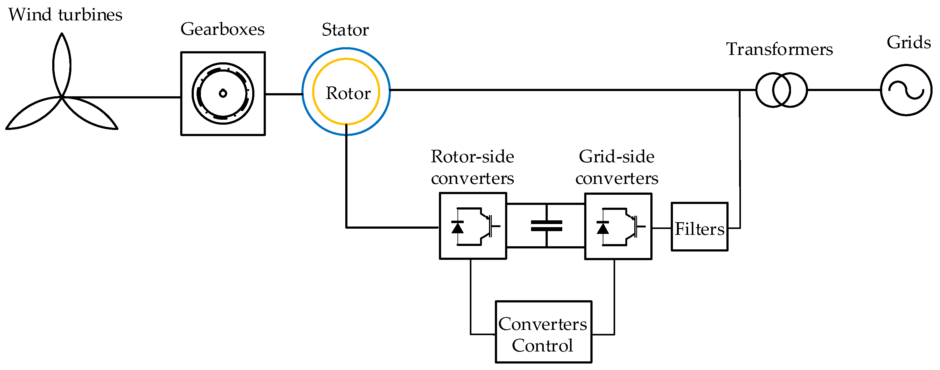
2. The Mathematical Model of DFIG

The structure diagram of a doubly-fed induction wind turbine, shown in Figure 1, consists of five main parts: wind turbine, gearbox, doubly-fed induction generator, back-to-back converter, and converter control system [19]. The basic working principle is that the wind drives the wind turbine, converting wind energy into mechanical energy, and the gearbox drive system drags the doubly-fed induction generator to generate a three-phase alternating current with alternating frequency and amplitude to the grid. The wind turbine is linked to the doubly-fed induction generator by the gearbox drive system. The stator side of the generator is attached directly to the grid, while the rotor side is connected to a back-to-back converter to the grid, which enables the stator and rotor to transport power from the grid in both directions [20]. The grid-side converter is to ensure the quality of the power output from the stator winding, and the rotor-side converter is to ensure that the rotor is adjustable and controllable to effectively complete the control strategy by adjusting the DFIG electromagnetic torque for the purpose of speed control [21].

The doubly-fed motor is a high-order, non-linear, strongly coupled multivariable, and parametrically time-varying system. Therefore, idealistic assumptions are usually made before analysis, and the mathematical model of the DFIG in a dq two-phase rotating coordinate system is shown below.

(1)

Voltage equation:

$$\{\begin{array}{l}{u}_{ds}=-R_s{i}_{ds}+\omega {\psi }_{qs}-p{\psi }_{ds}\\ u_{qs}=-R_s{i}_{qs}-\omega {\psi }_{ds}-p{\psi }_{qs}\\ u_{dr}=R_r{i}_{dr}-(\omega -{\omega }_r){\psi }_{qr}+p{\psi }_{dr}\\ u_{qr}=R_r{i}_{qr}+(\omega -{\omega }_r){\psi }_{dr}+p{\psi }_{qr}\end{array}$$

(1)

where $u_{ds}$, $u_{qs}$, $u_{dr}$, $u_{qr}$ are the components of the stator and rotor voltages on the d and q axes, $\omega$ is the stator angular velocities, ${\omega }_r$ is the rotor angular velocities, ${\omega }_s=\omega -{\omega }_r$ is the differential angular velocities and $p$ is the differential operators.

(2)

Magnetic chain equation:

$$\{\begin{array}{l}{\psi }_{ds}=L_s{i}_{ds}-L_m{i}_{dr}\\ {\psi }_{qs}=L_s{i}_{qs}-L_m{i}_{qr}\\ {\psi }_{dr}=-L_m{i}_{ds}+L_r{i}_{dr}\\ {\psi }_{qr}=-L_m{i}_{qs}+L_r{i}_{qr}\end{array}$$

(2)

In which, ${\psi }_{ds}$, ${\psi }_{qs}$, ${\psi }_{dr}$, ${\psi }_{qr}$ are the stator, rotor magnetic chain in the d, q axis of the component; $i_{ds}$, $i_{dr}$, $i_{qs}$, $i_{qr}$ are the stator, rotor current in the d, q axis of the component; $L_m$ is the stator-rotor mutual inductance; $L_s$, $L_r$ are the stator-rotor self-inductance.

Taking Equation (2) into Equation (1) gives the following relationship between current and voltage:

$$\left[\begin{array}{l}{u}_{ds}\\ u_{qs}\\ u_{dr}\\ u_{qr}\end{array}\right]=\left[\begin{array}{cccc}-R_s-L_{s}P& \omega L_s& L_{m}P& -\omega L_m\\ -\omega L_s& -R_s-L_{s}P& \omega L_m& L_{m}P\\ L_{m}P& {\omega }_s{L}_m& R_r+L_{r}P& -{\omega }_s{L}_r\\ -{\omega }_s{L}_m& -L_{m}P& {\omega }_s{L}_r& R_r+L_{r}P\end{array}\right]\left[\begin{array}{l}{i}_{ds}\\ i_{qs}\\ i_{dr}\\ i_{qr}\end{array}\right]$$

(3)

It can be seen from Equation (3) that the output current is related to the stator resistance, rotor resistance, stator inductance, rotor inductance, and stator-rotor mutual inductance for a constant input voltage.

(3)

Electromagnetic torque, power equation

The equations of motion are the same as in the three-phase stationary coordinate system, and the expression for the electromagnetic torque is:

$$T_e=n_p{L}_m(i_{ds}{i}_{qr}-i_{qs}{i}_{dr})=n_p({\psi }_{qs}{i}_{ds}-{\psi }_{ds}{i}_{qs})$$

(4)

The stator active and reactive power are:

$$\{\begin{array}{l}{P}_s=u_{ds}{i}_{ds}+u_{qs}{i}_{qs}\\ Q_s=u_{qs}{i}_{qs}-u_{ds}{i}_{ds}\end{array}$$

(5)

The rotor active and reactive power are:

$$\{\begin{array}{l}{P}_r=u_{dr}{i}_{dr}+u_{qr}{i}_{qr}\\ Q_r=u_{qr}{i}_{qr}-u_{dr}{i}_{dr}\end{array}$$

(6)

From Equations (1) to (6) it can be seen that $R_s$, $R_r$, $L_s$, $L_r$ and $L_m$ affect the output of the motor.

3. Algorithm Introduction

3.1. Grey Wolf Algorithm

The grey wolf optimization algorithm (GWO) was proposed by the scholar Seyedali Mirjalili [22] through observations of predators hunting in nature. The grey wolf optimization algorithm is a simple and implementable model that performs as well as other meta-heuristic swarm intelligence algorithms in many areas of optimization. Similar to other smart algorithms, the best solution is represented by the prey, and each possible solution is represented by each grey wolf. In the search for prey, grey wolves are endowed with a ranking depending on the quality of the calculated value of the adaptation function. The grey wolf has the optimum adaptation function score $\alpha$ wolf, the next best is $\beta$ wolf, the next best is $\delta$ wolf, and the rest are all $\omega$ wolves. $\alpha$, $\beta$, and $\delta$ wolves are much closer to their prey. The grey wolf’s level guidelines play an integral part in the hunting. The whole group of grey wolves is commanded by $\alpha$ wolf; $\beta$ wolf, also known as the deputy leader, follows the orders of $\alpha$ wolf, facilitates $\alpha$ wolf in deciding, and has jurisdiction over other wolves except $\alpha$ wolf; $\delta$ wolf, known as the ordinary wolf, follows the orders of wolves $\alpha$ and $\beta$, and acts as a sentry and scout; $\omega$ wolf, known as the bottom wolf, is not of high level but are numerous. The pack, led by wolf $\alpha$, surrounds the prey, wolves $\beta$ and $\delta$ attack the prey, and wolves d assist throughout the attack and eventually capture the prey.

The process of enveloping can be expressed as

$$D=\left|C\times X_P(t)-X(t)\right|$$

(7)

$$X(t+1)=X_P(t)-A\times D$$

(8)

where $X_P(t)$ is the position of the prey, $X$ denotes the position vector of the grey wolf, and $t$ is the current iteration. $C$ and $A$ are the coefficient vectors computed via Equations (9) and (10) below:

$$A=2\times A\times r_1-a$$

(9)

$$C=2\times r_2$$

(10)

where $r_1$, $r_2$ are random vectors in [0,1] and the elements of the $a$-vector decrease linearly from 2 to 0 during the iterative process according to the following Equation (11):

$$a=2-2(2\times t)/MaxIter$$

(11)

The hunting process can be expressed as follows:

$$D_{\alpha }=\left|C_1\times X_a-X(t)\right|$$

(12)

$$D_{\beta }=\left|C_2\times X_{\beta }-X(t)\right|$$

(13)

$$D_{\delta }=\left|C_3\times X_{\delta }-X(t)\right|$$

(14)

Here $C_1$, $C_2$, and $C_3$ are calculated by Equation (10) above:

$$X_{i1}(t)=X_{\alpha }(t)-A_{i1}\times D_{\alpha }(t)$$

(15)

$$X_{i2}(t)=X_{\beta }(t)-A_{i2}\times D_{\beta }(t)$$

(16)

$$X_{i3}(t)=X_{\delta }(t)-A_{i3}\times D_{\delta }(t)$$

(17)

$$X(t+1)=\frac{X_{i1}(t)+X_{i2}(t)+X_{i3}(t)}{3}$$

(18)

where $D_{\alpha }$, $D_{\beta }$ and $D_{\delta }$ are the distances of $\alpha$ wolf, $\beta$ wolf, and wolf $\delta$ from other wolves, respectively; $X_{\alpha }(t)$, $X_{\beta }(t)$, and $X_{\delta }(t)$ are the locations of wolves $\alpha$, $\beta$, and $\delta$, respectively; $A_{i1}$, $A_{i2}$, and $A_{i3}$ are coefficient vectors; $C_1$, $C_2$, and $C_3$ are random vectors, and $X$ is the current location of the individual wolf.

Finally, the wolves start to attack the prey and the value of $a$ in Equation (11) decreases linearly from 2 to 0 with time t. When $A\le 1$, the wolves concentrate on attacking the prey, focusing on the local search; when $A>1$, the wolves give up the pursuit of the current prey and disperse, focusing on the global search.

3.2. Adaptive Grey Wolf Algorithm Based on Information-Sharing Search Strategy (ISIAGWO)

The basic GWO algorithm has some advantages in terms of its optimality-finding ability when solving low-dimensional problems. As the complexity of the problem increases, the algorithm suffers from a reduction in population diversity and a lack of conditioning in the later stages of the linear convergence operator $a$, leading to a tendency for the algorithm to fall into local optima and insufficient solution efficiency [23,24]. To address these issues, Wu et al. [25] introduced iterative mapping, non-linear dynamic operators, and information-sharing search strategies to enhance the population diversity of the algorithm and balance the global and local search capabilities of the algorithm to improve the initial algorithm.

The standard iterative chaos mapping function is:

$$x_{k+1}=\sin \frac{b\pi }{x_k}$$

(19)

where the random number $b\in (0,1)$, taken as $b=0.5$ in this paper; $x_k$ is the value of the $k$th iteration $x$.

In the standard GWO algorithm, the convergence operator $a$ is linearly decreasing, making the local search capability of the algorithm significantly reduced in the later stages. The overall search performance of the algorithm is key to the algorithm, and putting down an incomplete gamma function to update the convergence operator $a$ effectively improves the global and local search performance of the algorithm [26] with the expression:

$$a=a_{lb}+\frac{a_{ub}-a_{lb}}{\lambda }\times gamma(\lambda ,1-\frac{t}{I_{max}})$$

(20)

where $a_{ub}$ and $a_{lb}$ are the upper and lower bounds of $a$, respectively; $t$ is the current number of iterations of the algorithm; $I_{max}$ is the maximum number of iterations, and $\lambda$ is the random number, which is taken as $\lambda =0.01$.

A new search strategy is proposed based on the connotation of information-sharing theory, including three steps information initialization, information sharing and information updating.

Initialization phase of wolf information: random distribution of wolves in a given search space, as specified by the expression:

$$X_{ij}=l{b}_j+k\times (s_{ubj}-s_{lbj})\begin{array}{cc}& i\in [1,N],j\in [1,D^{\prime }]\end{array}$$

(21)

where $s_{ubj}$ and $s_{lbj}$ are the upper and lower bounds of the search space; $k$ are the random numbers of the interval $(0,1)$; $N$ are the number of populations, and $D^{\prime }$ are the dimensions of the problem. The position of the $i$ wolf in the $t$ iteration can be obtained as $X_i(t)=\{X_{i1},X_{i2},●●●,X_{iD}\}$, and the degree of adaptation is denoted by $F(X_i(t))$.

Wolf pack information-sharing phase: each wolf acts as a candidate solution and shares information with nearby wolves, which can be represented as:

$$N_i(t)=\{X_j(t)|E_i(X_i(t),X_j(t)\le R_i(t),X_j(t)\in P_{pop}\}$$

(22)

where $E_i$ is the Euclidean distance between $X_i(t)$ and $X_j(t)$; $R_i(t)$ is the Euclidean distance between the current wolf location $X_i(t)$ and the candidate wolf $X_i(t+1)$, and $P_{pop}$ is the overall population size.

From the above, it can be seen that the information-sharing environment of the wolf pack has been successfully constituted, where the domain of individuals is constructed according to Equation (22). The candidate solutions for the wolf pack through dimensional information-sharing are as follows:

$$X_{i-IS,d}(t+1)=X_{i,d}(t)+r_{rand}\times (X_{n,d}(t)-X_{r,d}(t))$$

(23)

where $X_{i,d}(t)$ is the current individual; $X_{n,d}(t)$ is a random individual; $X_{r,d}(t)$ is another randomly selected individual in the population; $X_{i-IS,d}(t+1)$ is an individual updated by the information-sharing search strategy; $r_{rand}$ is a random number between [0,1].

Wolf information update phase: $X_{i-IS}(t+1)$ and $X_i(t+1)$ are compared in terms of fitness values and the better individual is selected, with the following update formula:

$$X_i(t+1)=\{\begin{array}{l}{X}_i(t+1)\begin{array}{cc}& f(X_i(t+1))<f(X_{i-IS}(t+1))\end{array}\\ X_{i-IS}(t+1)\begin{array}{cc}& \mathrm{Others}\end{array}\end{array}$$

(24)

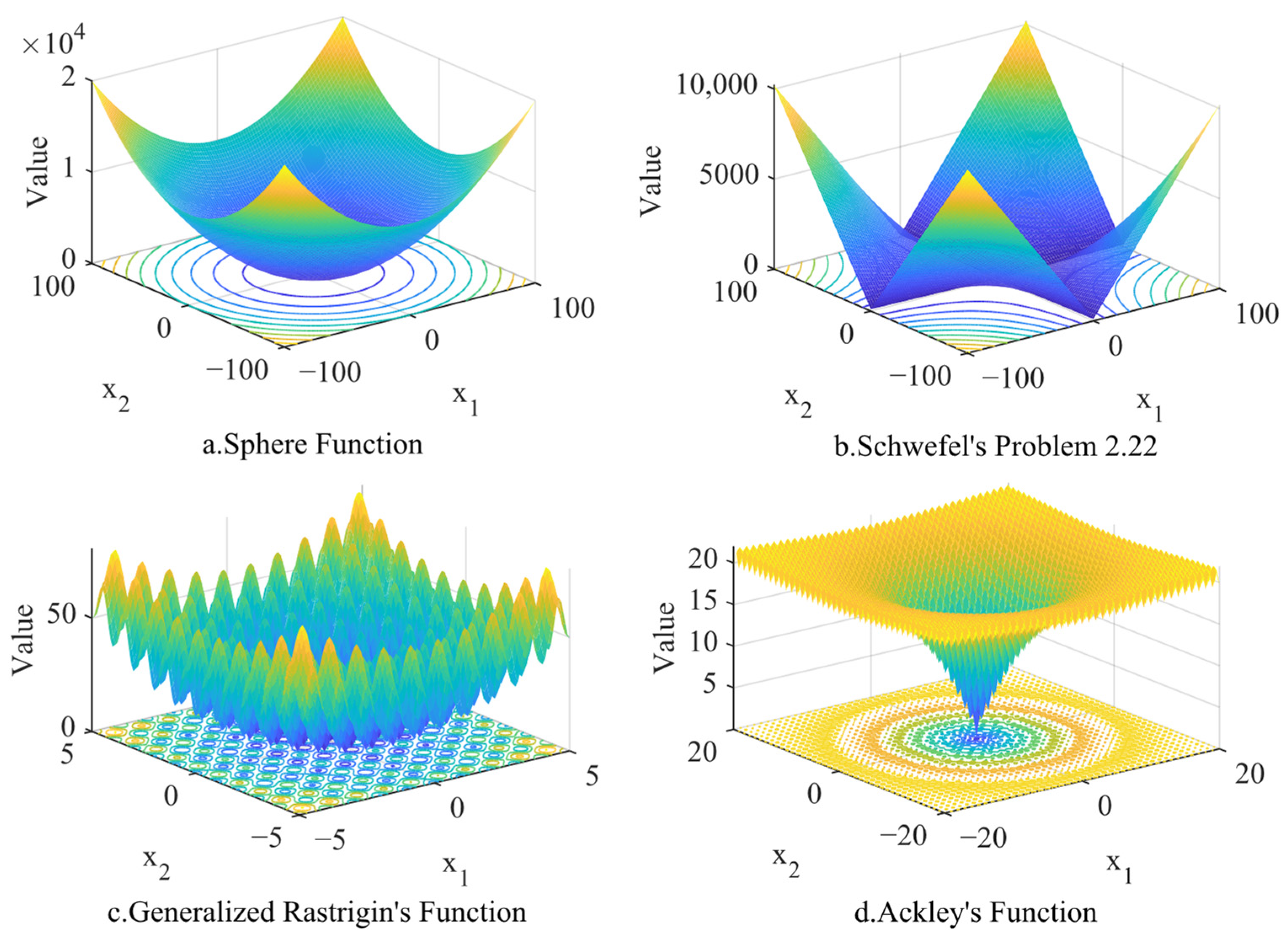
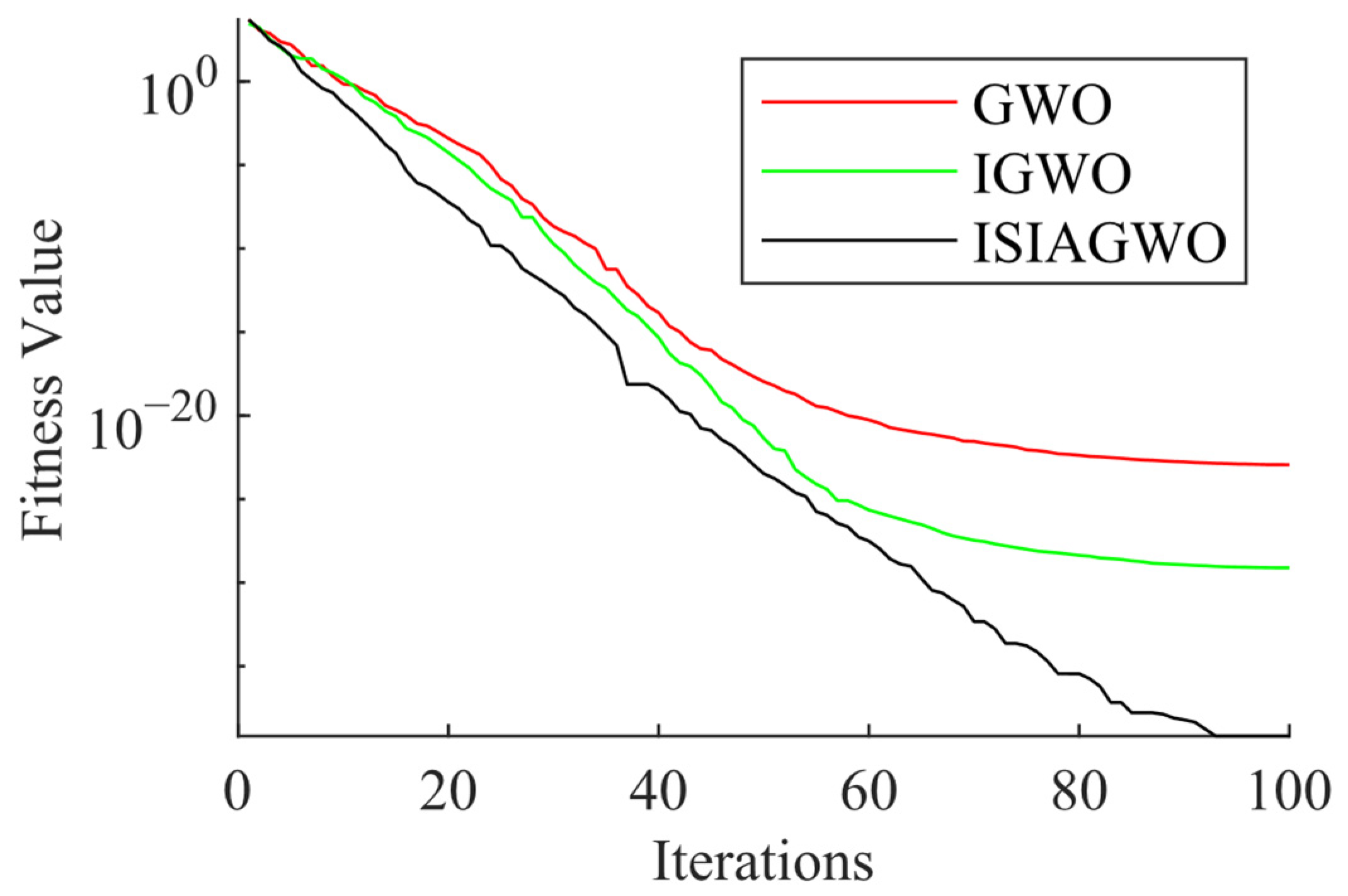
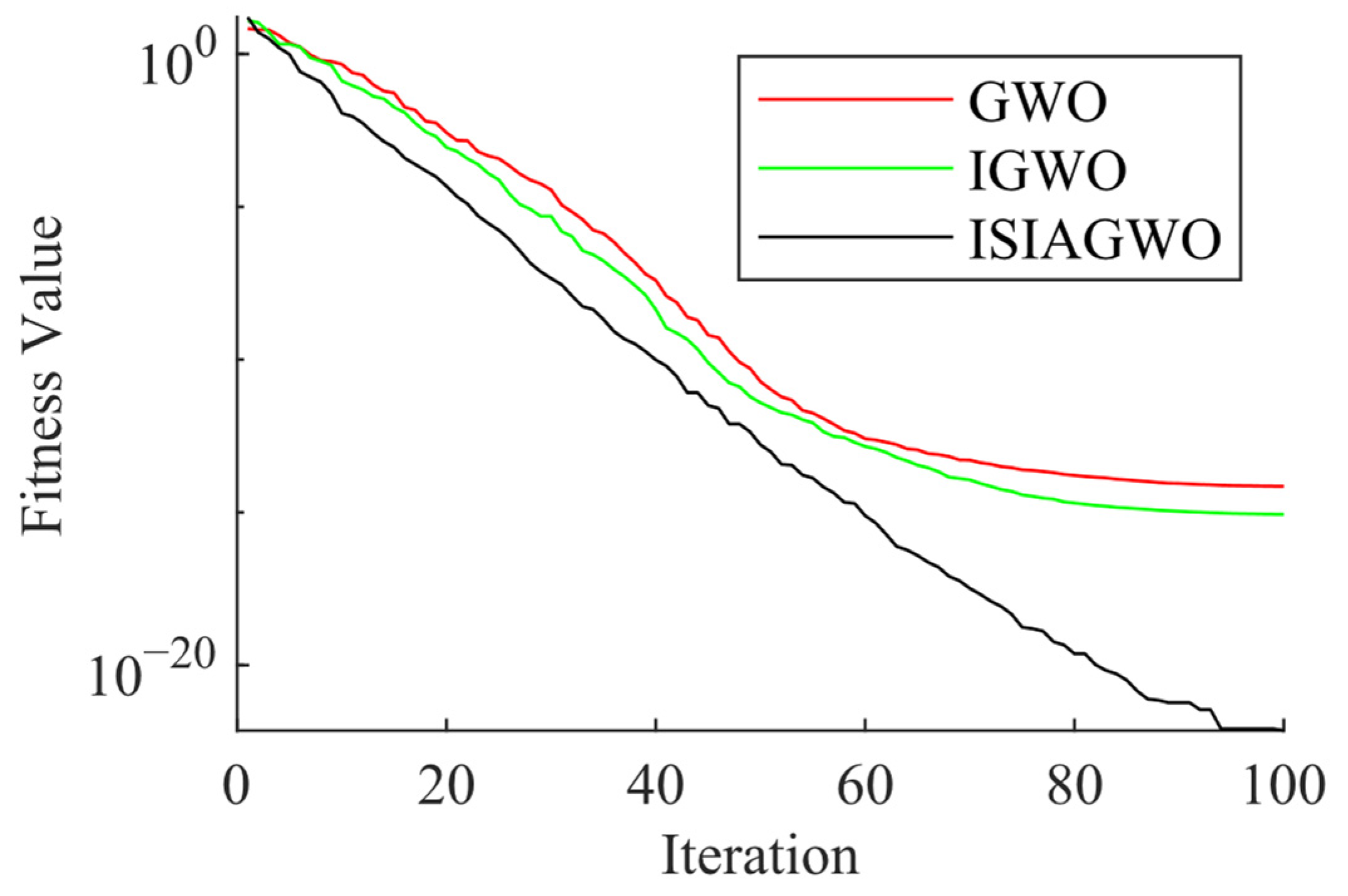
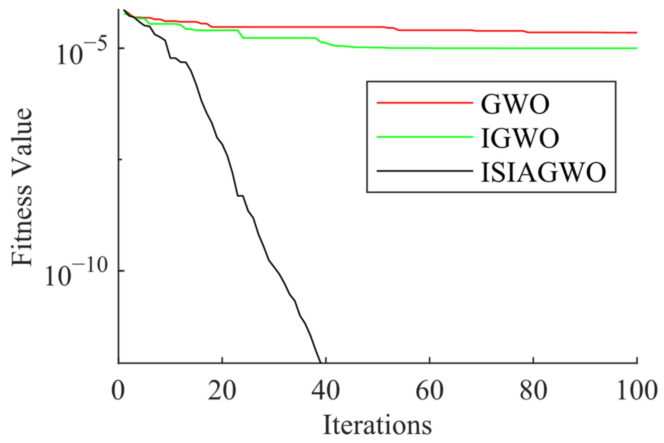
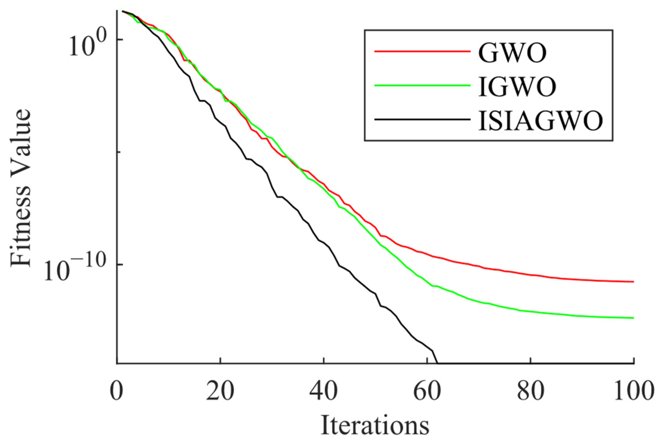
3.3. Algorithm Performance Test

In order to verify the performance of the ISIAGWO algorithm, four basic test functions are used in this paper, and the three algorithms of GWO and IGWO [27] to compare and verify, as shown in

Table 1. Standard test functions.

Name of Function	Functions	Value Range	Optimum
Sphere Function	$f_1(x)={\displaystyle \sum _{i=1}^n{x}_i^2}$	[−100, 100]	0
Schwefel’s Problem 2.22	$f_2(x)={\displaystyle \sum _{i=1}^{30}\left|xi\right|+{\displaystyle \prod _{i=1}^{30}\left|xi\right|}}$	[−10, 10]	0
Generalized Rastrigin’s Function	$f_3(x)={\displaystyle \sum _{i=1}^{30}[x_i^2-10\cos (2\pi x_i)+10]}$	[−5.12, 5.12]	0
Generalized Griewank’s Function	$\begin{array}{c}{f}_4(x)=-20\exp (-0.2\sqrt{\frac{1}{30}{\displaystyle \sum _{i=1}^{30}{x}_i^2}})-\\ \exp (\frac{1}{30}{\displaystyle \sum _{i=1}^{30}\cos 2\pi xi})+20+e\end{array}$	[−32, 32]	0

.

Among them, functions $f_1$ and $f_2$ are single-peaked functions, which are used to check the algorithm’s local optimization performance, and functions $f_3$ and $f_4$ are multi-peaked functions, which are used to check the algorithm’s global optimization capability. The optimal global values of the above four functions are all 0. The images of the test function are shown in Figure 2 below.

The parameters of the above three algorithms were all set to 30 dimensions, 50 populations, and 100 iterations, and the resulting optimization curves for the four functions are shown in Figure 3, Figure 4, Figure 5 and Figure 6 below.

The results of the three algorithm run, with their optimal values, mean values, and variance, are shown in

Table 2. Results of the algorithm test.

Functions	GWO			IGWO			ISIAGWO
	Optimum	Mean	Variance	Optimum	Mean	Variance	Optimum	Mean	Variance
$f_1$	2.286 × 10−21	6.680 × 101	4.357 × 102	7.842 × 10−24	6.775 × 101	4.494 × 102	6.679 × 10−42	2.654 × 101	1.639 × 102
$f_2$	2.580 × 10−13	4.817 × 10−1	2.082	2.681 × 10−15	4.532 × 10−1	3.107	4.228 × 10−22	3.406 × 10−1	1.886
$f_3$	4.979	9.456	6.765	9.950× 10−1	3.987	6.235	0.000	1.531	6.168
$f_4$	1.737× 10−11	7.779× 10−1	2.888	4.232× 10−13	7.137× 10−1	2.801	3.997× 10−15	6.900× 10−1	2.697

.

As can be seen from the test function optimization curves in Figure 3, Figure 4, Figure 5 and Figure 6, the convergence speed and the optimization effect of the ISIAGWO algorithm are significantly better than those of the original GWO and IGWO algorithms, and the optimal value, mean value, and variance of the ISIAGWO algorithm are better than those of the other two algorithms as can be seen from Table 2.

4. DFIG Parameter Identification

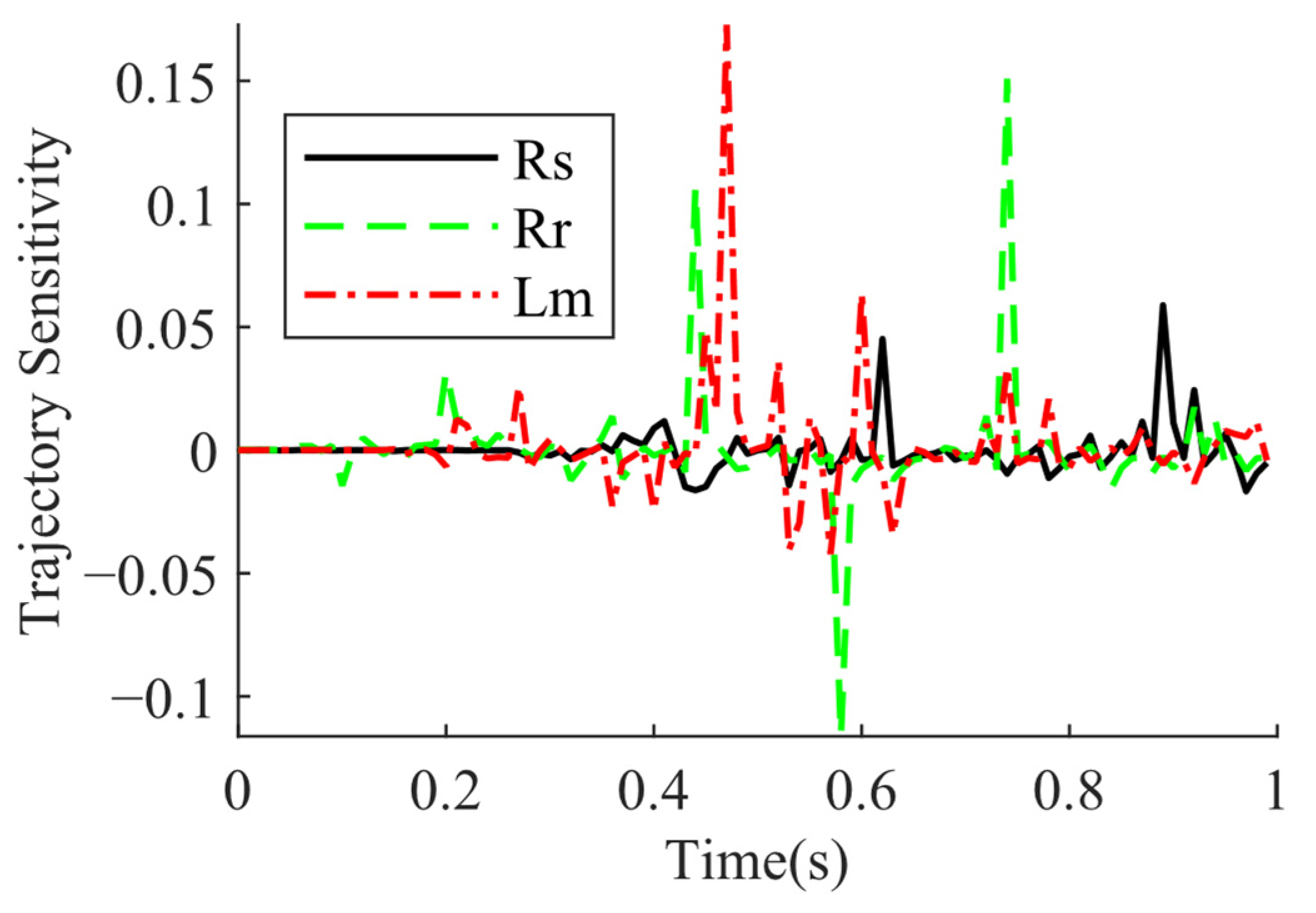
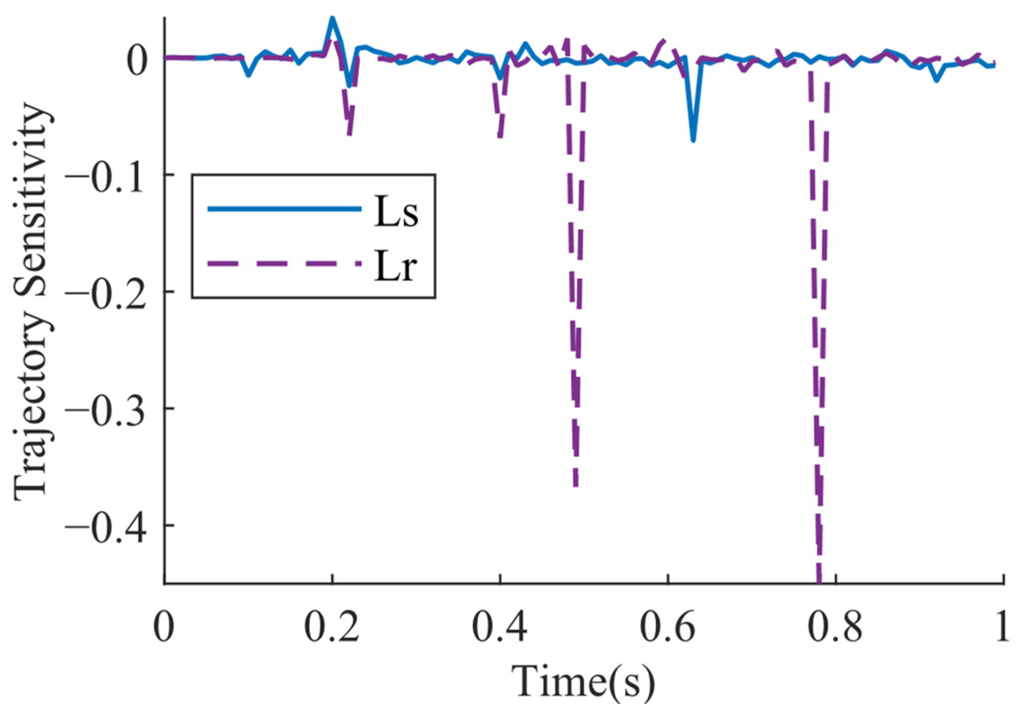
4.1. Identifiability of the Parameters

Before parameter identification can be carried out, it is necessary to know the identifiability of the parameters and the ease of parameter identification. The literature [28] suggests that trajectory sensitivity can be used to measure the identifiability of parameters and the ease of parameter identification. If the trajectory sensitivities of several parameters pass the zero point at the same time, it can be determined that these parameters are not uniquely identifiable. If the sensitivity of all the parameters does not pass the zero point at the same time, then the parameters are uniquely identifiable, and the greater the trajectory sensitivity, the greater the impact on the dynamic behavior of the system and the easier it is to identify. The relative values of trajectory sensitivity are defined as follows:

$$S_{{\theta }_i}=\underset{\mathsf{\Delta }{\theta }_i\to 0}{\lim }\frac{\frac{y(t,{\theta }_1,\cdots ,{\theta }_i+\mathsf{\Delta }{\theta }_i,\cdots ,{\theta }_m)-y(t,{\theta }_1,\cdots ,{\theta }_i,\cdots ,{\theta }_m)}{y(t,{\theta }_1,\cdots ,{\theta }_i,\cdots ,{\theta }_m)}}{\frac{\mathsf{\Delta }{\theta }_i}{{\theta }_{i0}}}$$

(25)

where ${\theta }_i$ is the sensitivity parameter to be found; ${\theta }_{i0}$ is the given value of ${\theta }_i$ the parameter; $y$ is the observed trajectory; $\mathsf{\Delta }$ is the increment of the corresponding parameter.

This paper builds a system model based on the MATLAB/Simulink simulation platform for doubly-fed wind turbines connected to an infinite grid, as shown in Figure 7. A wind farm consisting of six wind turbines is connected through a 30 kM transmission line to a 25 kV distribution grid supplying power to a 120 kV grid.

Set the model parameters as shown in

Table 3. Parameters of the model.

Components	Parameters	Values
Doubly-fed generator	Stator resistance $R_s$ (p.u.)	0.023
	Stator inductors $L_r$ (p.u.)	0.180
	Rotor resistance $R_r$ (p.u.)	0.016
	Rotor inductors $L_r$ (p.u.)	0.160
	Stator-rotor mutual inductance $L_m$ (p.u.)	2.900
Wind Turbine	Rotor inertia time constant $H_g$ (s)	0.685
	Wind turbine inertia time constants $H_w$ (s)	4.320
	Damping factor of the shaft system $D_{sh}$ (p.u.)	1.110
	Shaft system stiffness factor $K_{sh}$ (p.u.)	1.500
	polar logarithms $P$	3.000
Grid	Grid voltage $U$ (kV)	120.000
	Grid capacity $S$ (MVA)	2500.000

.

In this example, the wind speed is set at 15 m/s, the speed is maintained at 1.2 p.u., the steady-state output power is 0.9 p.u., the simulation time is 1 s, when $t$ = 0.3 s, a transient three-phase short circuit fault occurs at the end of the transmission line, and the fault is eliminated at $t$ = 0.4 s. Using the fan outlet current as the observed quantity, increase $R_s$, $R_r$, $L_s$, $L_r$, and $L_m$ by 10% each, and keep the rest of the parameters unchanged, and calculate. The trajectory sensitivity is shown in Figure 8 and Figure 9 below.

It can be observed from Figure 8 that the three parameters $R_s$, $R_r$, and $L_m$ do not pass the zero point at the same time, which leads to the conclusion that the three parameters $R_s$, $R_r$, and $L_m$ are identifiable. As can be seen from Figure 9, the phases $L_s$ and $L_r$ are close to each other, but there are still some gaps that do not pass the zero point at the same time, which leads to the conclusion that the two parameters $L_s$ and $L_r$ are identifiable. In addition, after the end of the short circuit fault, the trajectory sensitivity curve of each parameter will also occur relatively large abrupt changes, indicating that the change of parameter values after the end of the short circuit fault in the grid will also have a certain impact on the response of the unit.

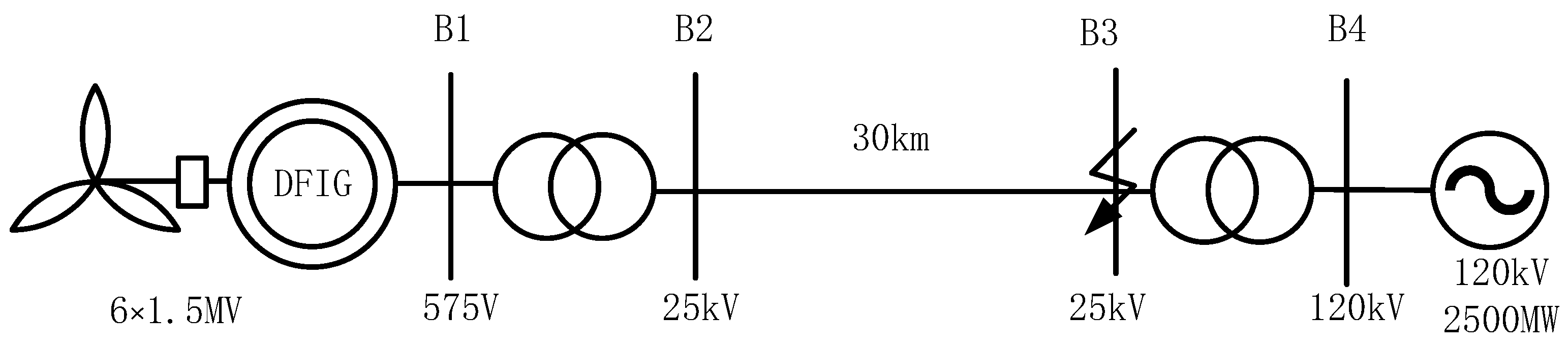
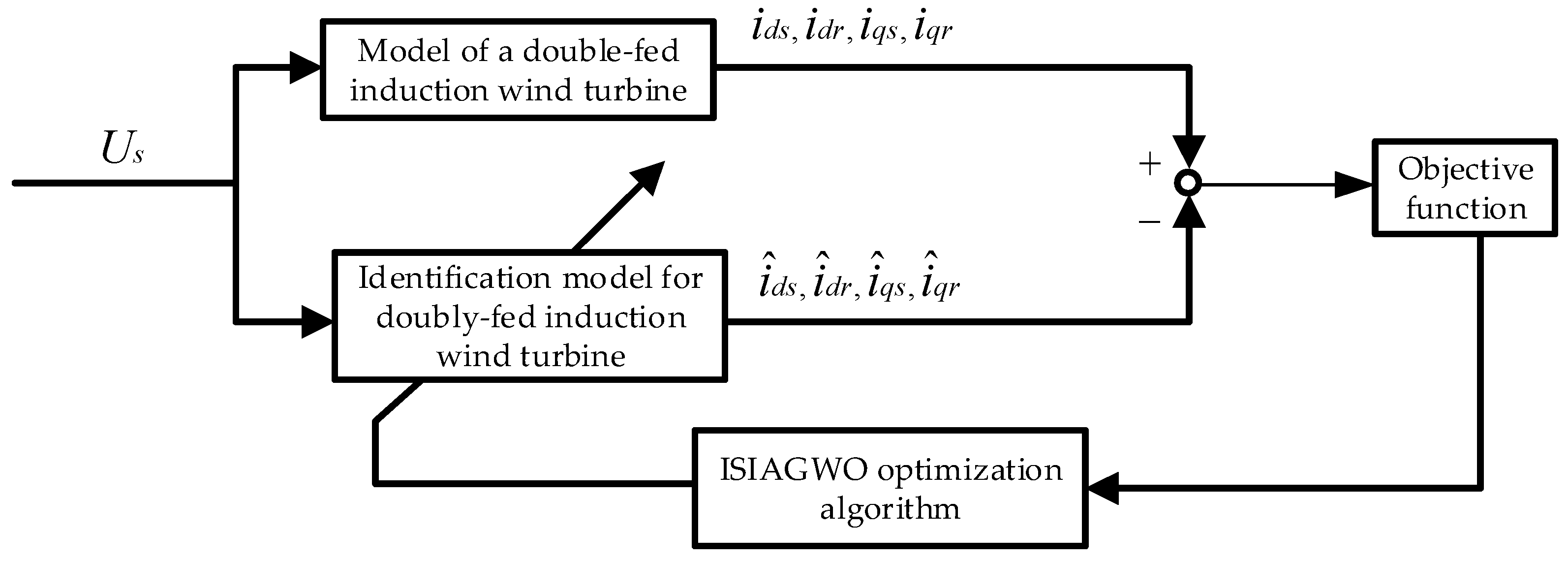
4.2. The DFIG Identification Model

When performing DFIG parameter estimation, the mathematical model of DFIG can be transformed into a state equation, as described in the literature [29], as shown in the following equation:

$$\begin{array}{l}\dot{x}(t)=f(P,x(t),u(t))\\ y(t)=g(P,x(t))\end{array}$$

(26)

In which, $x(t)$ is the state variable, $u(t)$ is the system input, $P$ is the DFIG parameter to be identified, and $y(t)$ is the system output.

In the DFIG identification model, $x(t)=(i_d,i_q)$, $u(t)=(u_d,u_q)$, $P=(R_s,R_r,L_s,L_r,L_m)$, $y(t)=(i_d,i_q)$. In order to identify the DFIG parameters $P$, the desired system state model is developed as follows:

$$\begin{array}{l}\widehat{\dot{x}}(t)=f(\widehat{P},\widehat{x}(t),u(t))\\ \widehat{y}(t)=g(\widehat{P},\widehat{x}(t))\end{array}$$

(27)

In the DFIG identification model, $\widehat{x}(t)=({\widehat{i}}_d,{\widehat{i}}_q)$, $u(t)=(u_d,u_q)$, $\widehat{P}=({\widehat{R}}_s,{\widehat{R}}_r,{\widehat{L}}_s,{\widehat{L}}_r,{\widehat{L}}_m)$, $\widehat{y}(t)=({\widehat{i}}_d,{\widehat{i}}_q)$. Suppose that the output error is defined as:

$$e=y-\widehat{y}$$

(28)

The degree of difference between the output of the desired system and the output of the actual system can then be expressed in terms of the following performance indicators:

$$f(P)={\displaystyle {\int }_{t1}^{t2}{e}^{T}edt}$$

(29)

is expressed in discrete form as:

$$f(P)={\displaystyle \sum _{K=1}^N\{{[y(k)-\widehat{y}(k)]}^T[y(k)-\widehat{y}(k)]\}}$$

(30)

Therefore, when building the DFIG multi-parameter identification model, the current and rotor speed of the doubly-fed motor are taken as state quantities, and the state equation of the DFIG can be derived according to the above Equation (30).

$$\{\begin{array}{l}\frac{{di}_{ds}}{dt}=-[((\omega -{\omega }_r)L_m^2-\omega L_s{L}_r)i_{qs}+R_s{L}_r{i}_{ds}-R_r{L}_m{i}_{dr}\\ \hspace{1em}\hspace{1em}-{\omega }_r{L}_r{L}_m{i}_{qr}-L_r{u}_{ds}+L_m{u}_{dr}]/\sigma L_s{L}_r\\ \frac{{di}_{qs}}{dt}=-[((\omega -{\omega }_r)L_m^2+\omega L_s{L}_r)i_{ds}+R_s{L}_r{i}_{qs}-R_r{L}_m{i}_{qr}\\ \hspace{1em}\hspace{1em}+{\omega }_r{L}_r{L}_m{i}_{dr}-L_r{u}_{qs}+L_m{u}_{qr}]/\sigma L_s{L}_r\\ \frac{{di}_{dr}}{dt}=-[-((\omega -{\omega }_r)L_s{L}_r-\omega L_m^2)i_{qr}-R_s{L}_m{i}_{ds}-R_r{L}_s{i}_{dr}\\ \hspace{1em}\hspace{1em}-{\omega }_r{L}_s{L}_m{i}_{qs}-L_s{u}_{dr}+L_m{u}_{ds}]/\sigma L_s{L}_r\\ \frac{{di}_{qr}}{dt}=-[((\omega -{\omega }_r)L_s{L}_r-\omega L_m^2)i_{dr}-R_s{L}_m{i}_{qs}+R_r{L}_s{i}_{qr}\\ \hspace{1em}\hspace{1em}-{\omega }_r{L}_s{L}_m{i}_{ds}-L_s{u}_{qr}+L_m{u}_{qs}]/\sigma L_s{L}_r\end{array}$$

(31)

where the leakage coefficient is $\sigma =1-L_m^2/L_s{L}_r$.

Let the sampling period be $T_s$, and discretize the above equation to obtain the actual system state equation:

$$\{\begin{array}{l}{i}_{ds}(k+1)=-[((\omega -{\omega }_r(k))L_m^2-\omega L_s{L}_r)i_{qs}(k)+R_s{L}_r{i}_{ds}(k)\\ \hspace{1em}\hspace{1em}\hspace{1em}\hspace{1em}-R_r{L}_m{i}_{dr}(k)-{\omega }_r(k)L_r{L}_m{i}_{qr}(k)-L_r{u}_{ds}(k)\\ \hspace{1em}\hspace{1em}\hspace{1em}\hspace{1em}+L_m{u}_{dr}(k)]T_s/\sigma L_s{L}_r+i_{ds}(k)\\ i_{qs}(k+1)=-[((\omega -{\omega }_r(k))L_m^2+\omega L_s{L}_r)i_{ds}(k)+R_s{L}_r{i}_{qs}(k)\\ \hspace{1em}\hspace{1em}\hspace{1em}\hspace{1em}-R_r{L}_m{i}_{qr}(k)+{\omega }_r(k)L_r{L}_m{i}_{dr}(k)-L_r{u}_{qs}(k)\\ \hspace{1em}\hspace{1em}\hspace{1em}\hspace{1em}+L_m{u}_{qr}(k)]T_s/\sigma L_s{L}_r+i_{qs}(k)\\ i_{dr}(k+1)=-[-((\omega -{\omega }_r(k))L_s{L}_r-\omega L_m^2)i_{qr}(k)-R_s{L}_m{i}_{ds}(k)\\ \hspace{1em}\hspace{1em}\hspace{1em}\hspace{1em}-R_r{L}_s{i}_{dr}(k)-{\omega }_r{L}_s{L}_m{i}_{qs}(k)-L_s{u}_{dr}(k)\\ \hspace{1em}\hspace{1em}\hspace{1em}\hspace{1em}+L_m{u}_{ds}(k)]T_s/\sigma L_s{L}_r+i_{dr}(k)\\ i_{qr}(k+1)=-[((\omega -{\omega }_r(k))L_s{L}_r-\omega L_m^2)i_{dr}(k)-R_s{L}_m{i}_{qs}(k)\\ \hspace{1em}\hspace{1em}\hspace{1em}\hspace{1em}+R_r{L}_s{i}_{qr}(k)-{\omega }_r(k)L_s{L}_m{i}_{ds}(k)-L_s{u}_{qr}(k)\\ \hspace{1em}\hspace{1em}\hspace{1em}\hspace{1em}+L_m{u}_{qs}(k)]T_s/\sigma L_s{L}_r+i_{qr}(k)\end{array}$$

(32)

Let ${\widehat{i}}_{ds}$, ${\widehat{i}}_{dr}$, ${\widehat{i}}_{qs}$, and ${\widehat{i}}_{qr}$, be the estimates of $i_{ds}$, $i_{dr}$, $i_{qs}$, and $i_{qr}$, respectively, and the equation of state under the desired system is as follows:

$$\{\begin{array}{l}{\widehat{i}}_{ds}(k+1)=-[((\omega -{\omega }_r(k))L_m^2-\omega L_s{L}_r){\widehat{i}}_{qs}(k)+R_s{L}_r{\widehat{i}}_{ds}(k)\\ \hspace{1em}\hspace{1em}\hspace{1em}\hspace{1em}-R_r{L}_m{\widehat{i}}_{dr}(k)-{\omega }_r(k)L_r{L}_m{\widehat{i}}_{qr}(k)-L_r{u}_{ds}(k)\\ \hspace{1em}\hspace{1em}\hspace{1em}\hspace{1em}+L_m{u}_{dr}(k)]T_s/\sigma L_s{L}_r+{\widehat{i}}_{ds}(k)\\ {\widehat{i}}_{qs}(k+1)=-[((\omega -{\omega }_r(k))L_m^2+\omega L_s{L}_r){\widehat{i}}_{ds}(k)+R_s{L}_r{\widehat{i}}_{qs}(k)\\ \hspace{1em}\hspace{1em}\hspace{1em}\hspace{1em}-R_r{L}_m{\widehat{i}}_{qr}(k)+{\omega }_r(k)L_r{L}_m\widehat{i}{d}_r(k)-L_r{u}_{qs}(k)\\ \hspace{1em}\hspace{1em}\hspace{1em}\hspace{1em}+L_m{u}_{qr}(k)]T_s/\sigma L_s{L}_r+{\widehat{i}}_{qs}(k)\\ {\widehat{i}}_{dr}(k+1)=-[-((\omega -{\omega }_r(k))L_s{L}_r-\omega L_m^2){\widehat{i}}_{qr}(k)-R_s{L}_m{\widehat{i}}_{ds}(k)\\ \hspace{1em}\hspace{1em}\hspace{1em}\hspace{1em}-R_r{L}_s{\widehat{i}}_{dr}(k)-{\omega }_r{L}_s{L}_m{\widehat{i}}_{qs}(k)-L_s{u}_{dr}(k)\\ \hspace{1em}\hspace{1em}\hspace{1em}\hspace{1em}+L_m{u}_{ds}(k)]T_s/\sigma L_s{L}_r+{\widehat{i}}_{dr}(k)\\ {\widehat{i}}_{qr}(k+1)=-[((\omega -{\omega }_r(k))L_s{L}_r-\omega L_m^2){\widehat{i}}_{dr}(k)-R_s{L}_m{\widehat{i}}_{qs}(k)\\ \hspace{1em}\hspace{1em}\hspace{1em}\hspace{1em}+R_r{L}_s{\widehat{i}}_{qr}(k)-{\omega }_r(k)L_s{L}_m{\widehat{i}}_{ds}(k)-L_s{u}_{qr}(k)\\ \hspace{1em}\hspace{1em}\hspace{1em}\hspace{1em}+L_m{u}_{qs}(k)]T_s/\sigma L_s{L}_r+{\widehat{i}}_{qr}(k)\end{array}$$

(33)

In the above mathematical model of DFIG, the motor parameter $\{R_s,R_r,L_s,L_r,L_m\}$ are the identification parameters, and according to Equation (30), the objective function of the system can be established as shown in Equation (34); then the parameter identification problem is transformed into the problem of finding the minimum value of Equation (34):

$$f(P)={\displaystyle \sum _{k=1}^N\begin{array}{l}(w_1{(i_{ds}(k)-{\widehat{i}}_{ds}(k))}^2+w_2{(i_{dr}(k)-{\widehat{i}}_{dr}(k))}^2\\ +w_3{(i_{qs}(k)-{\widehat{i}}_{qs}(k))}^2+w_4{(i_{qr}(k)-{\widehat{i}}_{qr}(k))}^2)\end{array}}$$

(34)

where $i_{ds}$, $i_{dr}$, $i_{qs}$, and $i_{qr}$ are the current values in the dq coordinate system measured in the actual model, ${\widehat{i}}_{ds}$, ${\widehat{i}}_{dr}$, ${\widehat{i}}_{qs}$, and ${\widehat{i}}_{qr}$ are the current values in the dq coordinate system calculated in the identification model, and $w_1$, $w_2$, $w_3$, and $w_4$ are the weights, each taken as 0.25.

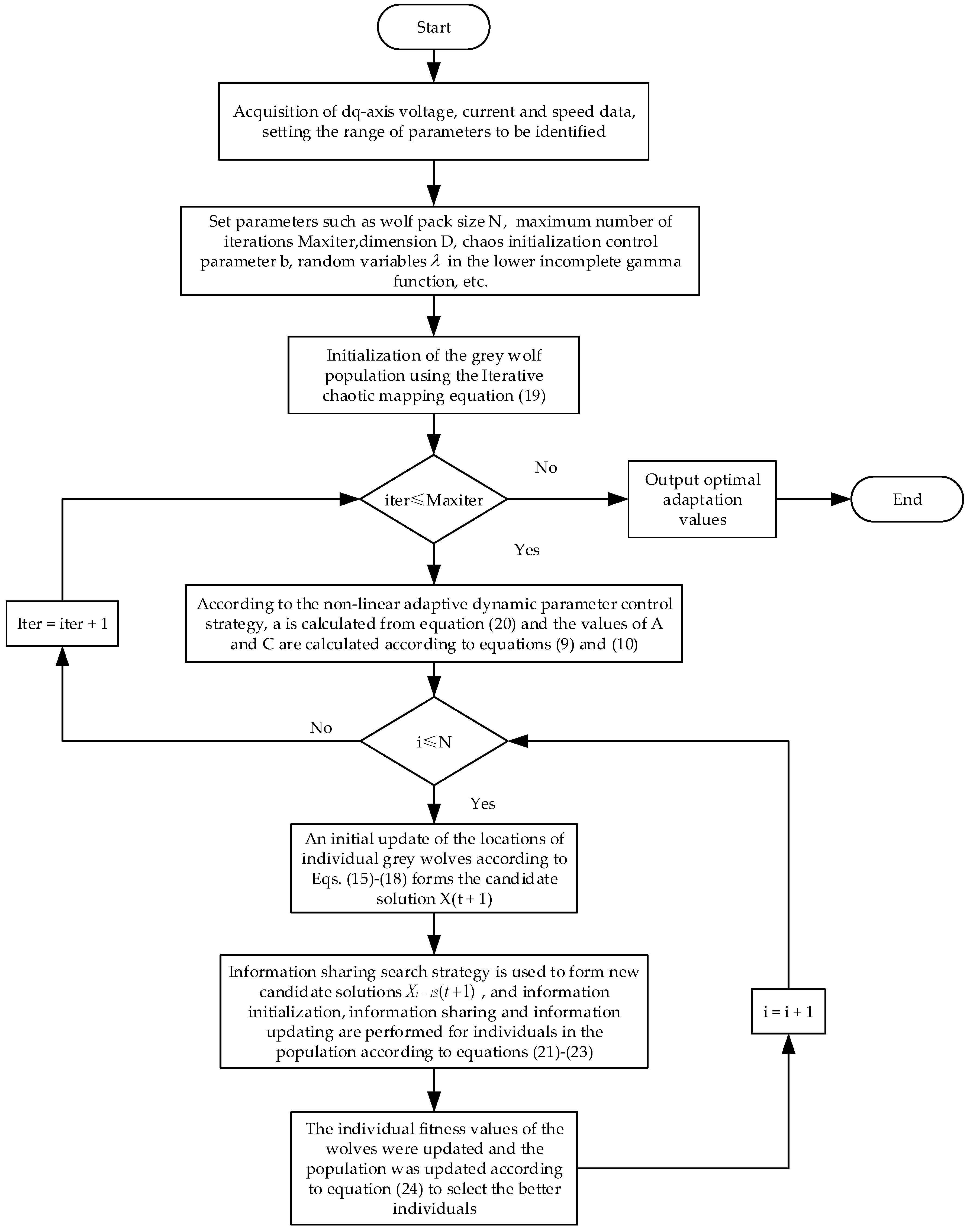
4.3. Principle and Steps of the ISIAGWO Algorithm for Identification

The DFIG parameter identification process is based on the difference between the actual output of the motor and the output of the identification model, and the identification model is continuously adjusted by the ISIAGWO algorithm to finally identify the DFIG parameters. The identification principle is shown in Figure 10.

The ISIAGWO algorithm was used to identify the DFIG parameters, and the flow chart is shown in Figure 11 below.

5. Simulation and Analysis

5.1. Parameter Settings

In the simulations of parameter identification, the initial values of the population particles of the three algorithms, all of which were randomly initialized within the initialization range of the given solution space, set the initial search interval for the motor parameters, as shown in

Table 4. True values of motor parameters and their initialization range.

Parameters	Initialization Range	True Value
Stator resistance $R_s(p.u.)$	0.01500~0.03200	0.02300
Rotor resistance $R_r(p.u.)$	0.01000~0.02200	0.01600
Stator inductors $L_s(p.u.)$	0.10000~0.22000	0.1800
Rotor inductors $L_r(p.u.)$	0.10000~0.22000	0.1600
Stator-rotor mutual inductance $L_m(p.u.)$	1.50000~5.00000	2.900

.

Each algorithm sets the number of populations to 10 and the maximum number of iterations to 100.

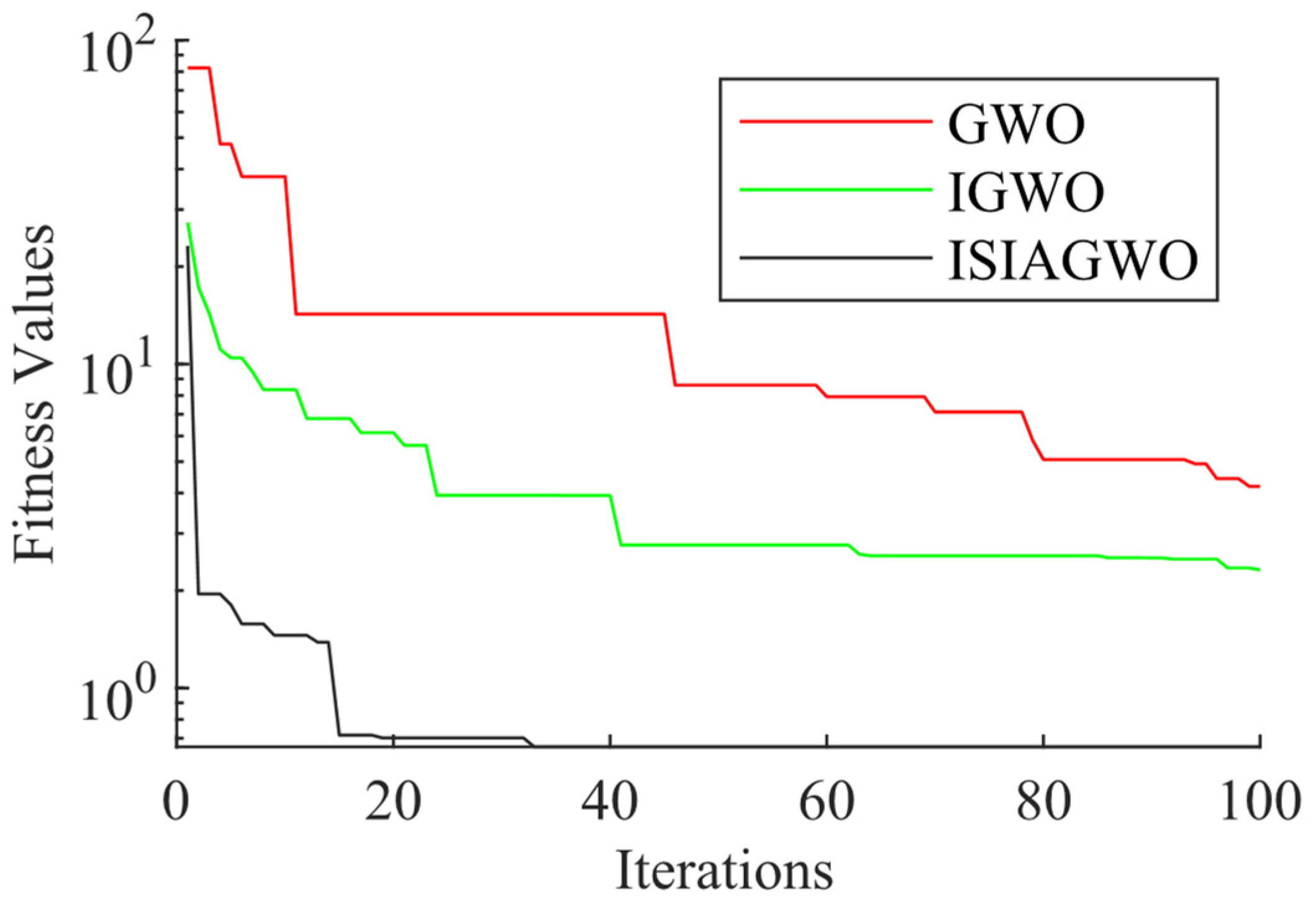
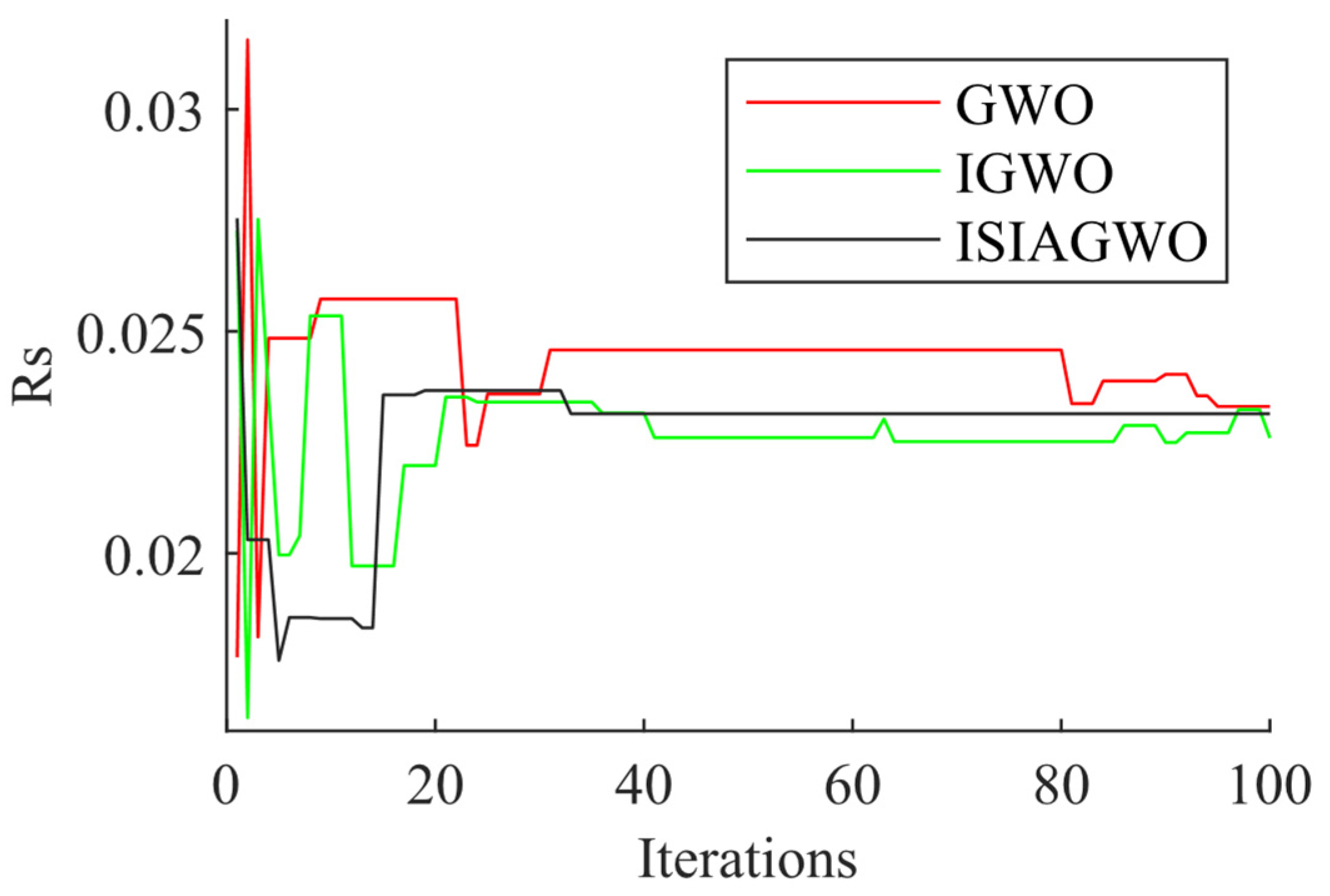
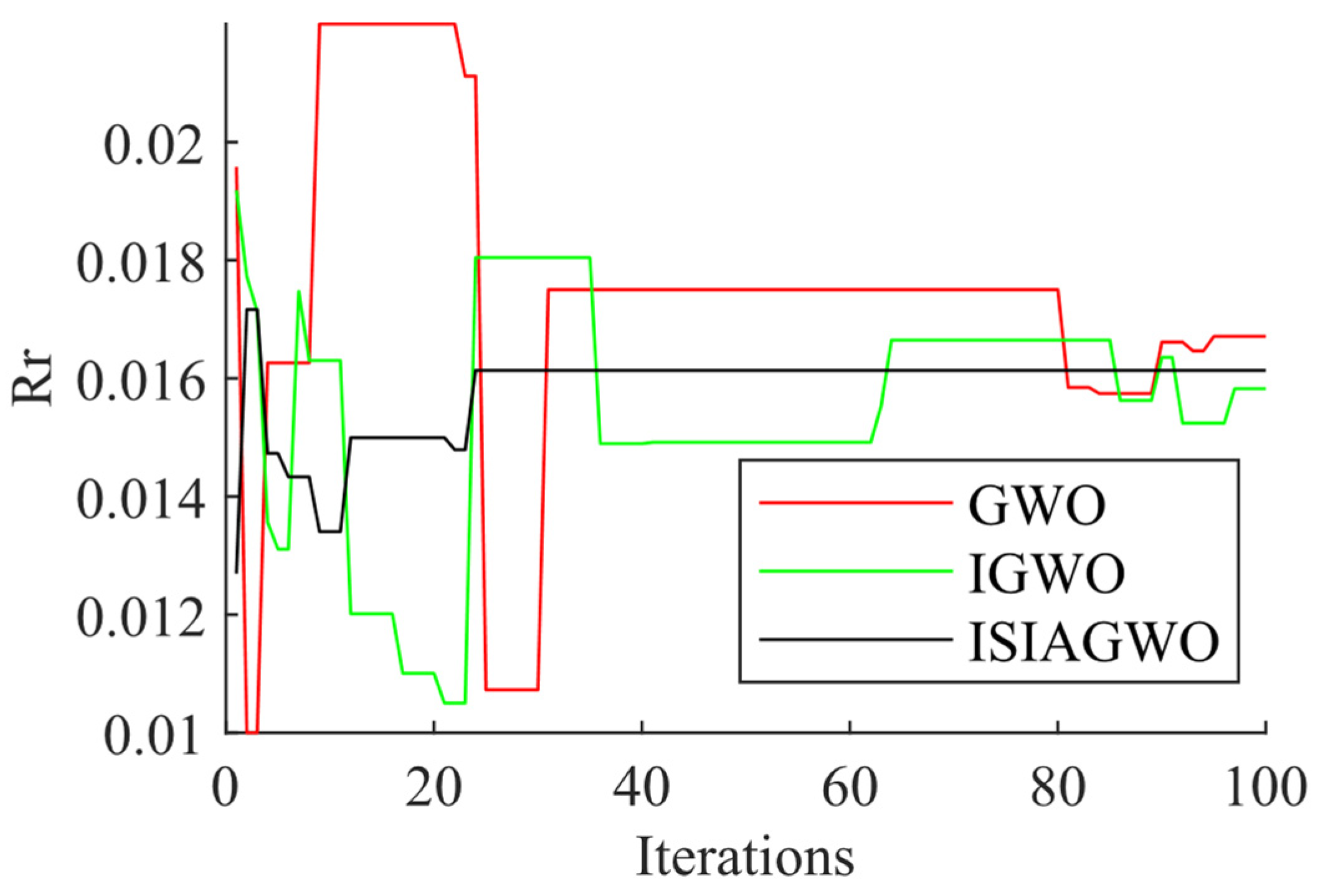
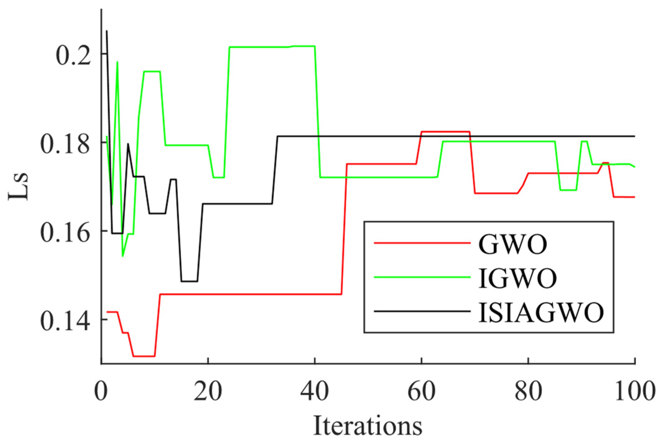
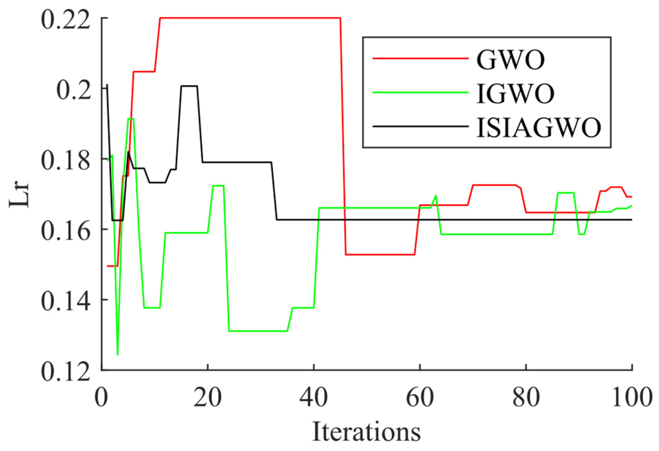
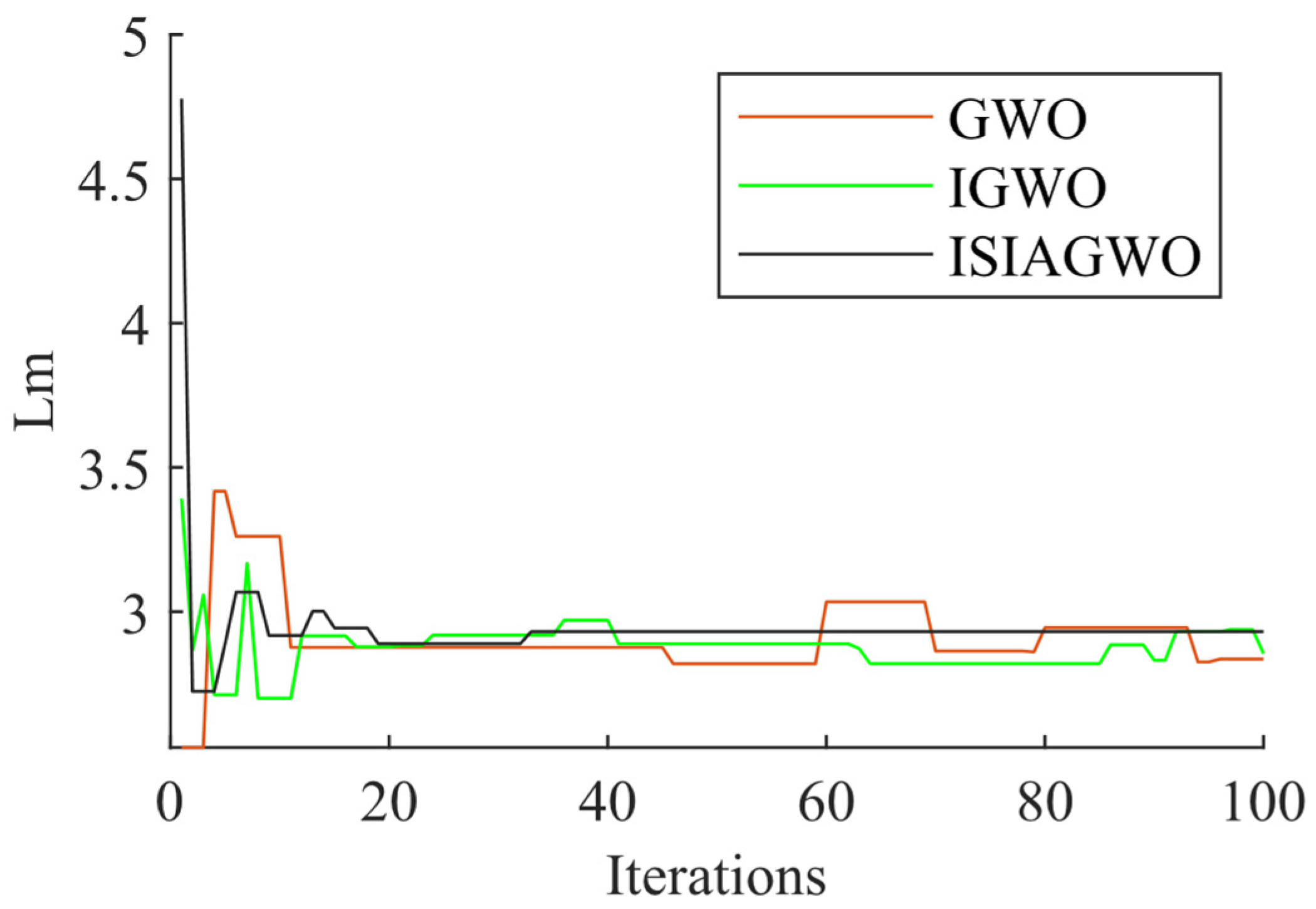
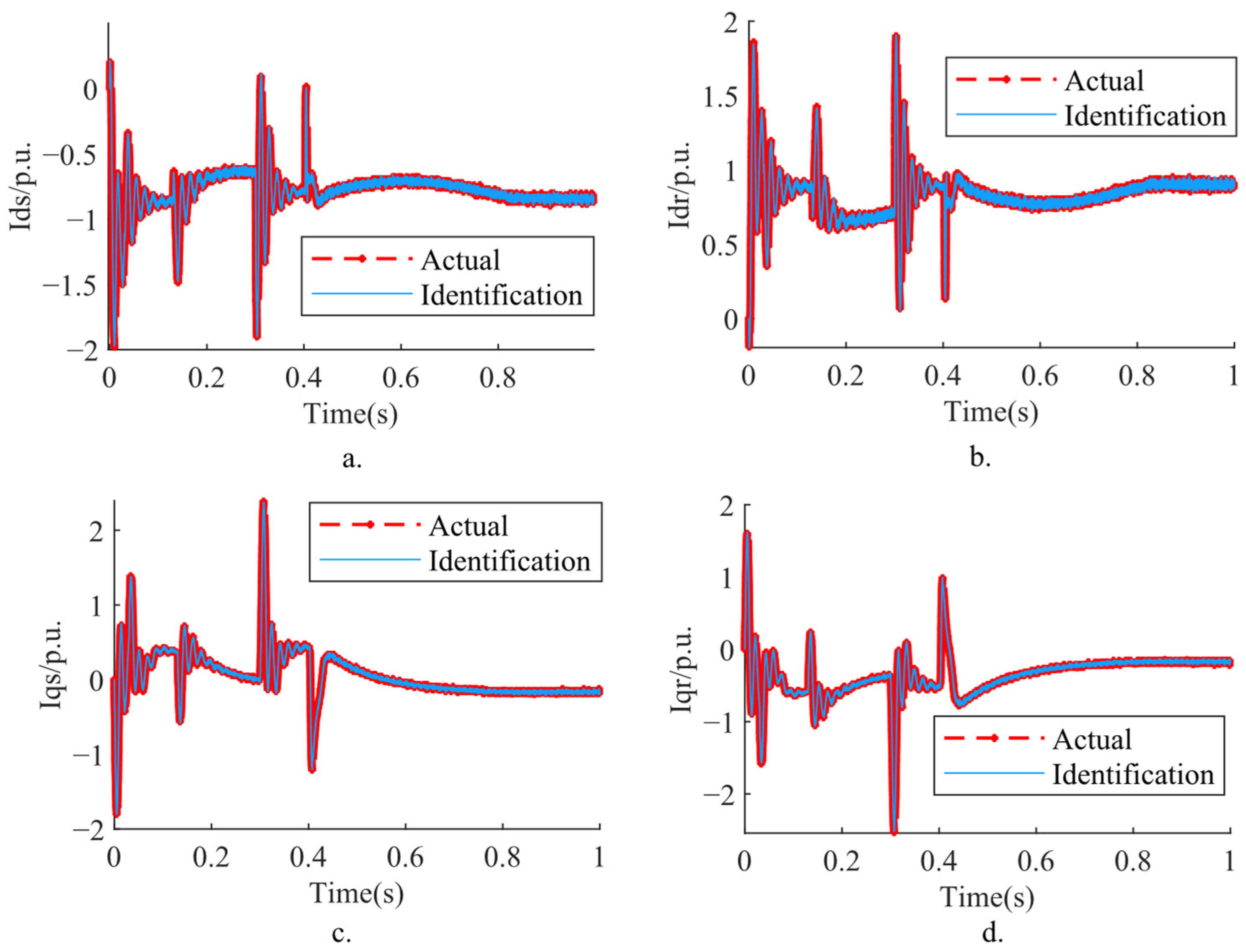
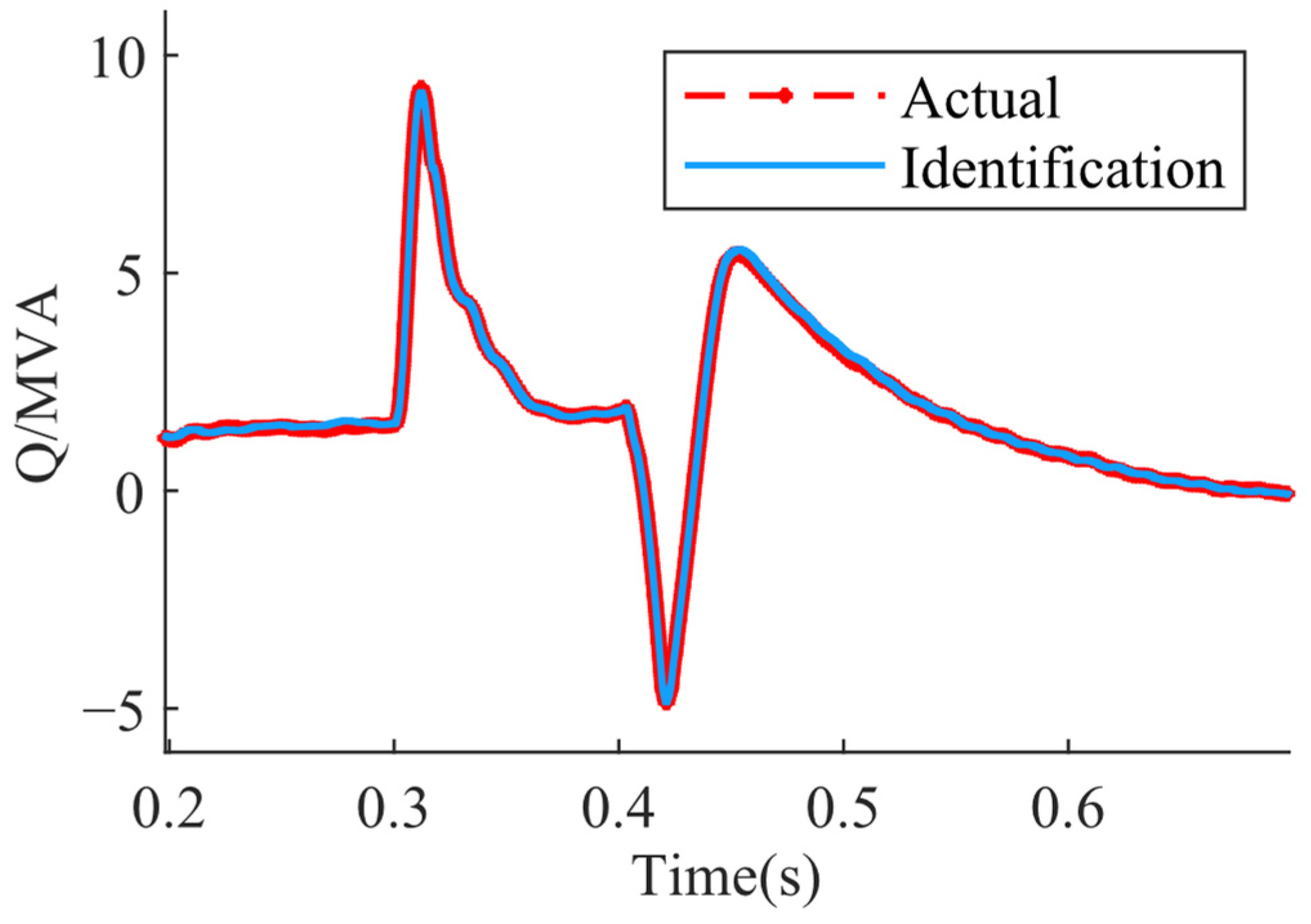
5.2. Results and Analysis

The results of the optimization of the three algorithms to identify adaptation are shown in

Table 5. Values of the fitness function for the three algorithms.

Algorithms	Minimum	Average	Variance
GWO	3.2388	9.0968	10.0749
IGWO	2.3159	4.3267	3.5354
ISIAGWO	0.6576	1.01616	2.26446

.

The results of the identification of $R_s$, $R_r$, $L_s$, $L_r$, and $L_m$ of the DFIG are shown in

Table 6. Comparison of the results of three algorithms for the identification of generator parameters.

Algorithms		$\mathit{R}\mathit{s}$	$\mathit{R}\mathit{r}$	$\mathit{L}\mathit{s}$	$\mathit{L}\mathit{r}$	$\mathit{L}\mathit{m}$
GWO	True value	0.02300	0.01600	0.18000	0.16000	2.90000
	Identifying value	0.02331	0.01671	0.16764	0.16921	2.83616
	Relative error%	−1.34%	−4.44%	6.87%	−5.75%	2.20%
IGWO	True value	0.02300	0.01600	0.18000	0.16000	2.90000
	Identifying value	0.02260	0.01582	0.17441	0.16671	2.85539
	Relative error%	1.75%	1.10%	3.11%	−4.19%	1.54%
ISIAGWO	True value	0.02300	0.01600	0.18000	0.16000	2.90000
	Identifying value	0.02314	0.01614	0.18137	0.16269	2.93127
	Relative error%	−0.63%	−0.85%	−0.76%	−1.68%	−1.08%

.

It can be observed from Table 5 that the ISIAGWO algorithm has smaller values of the fitness function compared to both the GWO algorithm and the IGWO algorithm. In terms of mean and minimum values, the ISIAGWO algorithm has better results in the parameter identification process, and in terms of variance, this algorithm is also more stable than the other two algorithms. It can be observed from Table 6, the ISIAGWO algorithm has better parameter identification accuracy than the other two algorithms and has the smallest error with the true value in the identification results for $R_s$, $R_r$, $L_s$, $L_r$, and $L_m$ of the DFIG.

The convergence curve of the DFIG’s parameter identification algorithm adaptation is shown in Figure 12.

The stator resistance of DFIG identification convergence curve, shown in Figure 13.

The rotor resistance of DFIG identification convergence curve, shown in Figure 14.

The stator inductance of DFIG identification convergence curve, shown in Figure 15.

The rotor inductance of DFIG identification convergence curve, shown in Figure 16.

The stator-rotor mutual inductance of DFIG identification convergence curve, shown in Figure 17.

From the convergence curves in Figure 13, Figure 14, Figure 15, Figure 16 and Figure 17, we can see that the GWO algorithm has the worst discrimination effect and the discrimination curve deviates from the true value the farthest. Compared with the GWO algorithm, the IGWO algorithm has a certain improvement in recognition accuracy, but the convergence speed of the two is almost the same; there is little difference. The ISIAGWO algorithm has the greatest recognition precision and convergence rate, as well as the highest parameter recognition results.

A comparison of the output of the actual model and the identification model in Figure 18, Figure 19 and Figure 20 shows that the differences are minimal, further illustrating the accuracy of the parameter identification results.

6. Conclusions

The analysis shows that the DFIG generator parameters have an influence on its output current, active, and reactive power. The analysis of the sensitivity of the generator parameter trajectory based on the observed quantity as the DFIG outlet current illustrates the identifiability of its parameters. The final simulation results show that the ISIAGWO algorithm can accurately identify the stator resistance, rotor resistance, stator inductance, rotor inductance, and stator-rotor mutual inductance, and its identification results are better than those of the GWO and IGWO algorithms, with better identification accuracy, stability, and convergence. The accuracy of the method can also be seen in the comparison between the output of the actual model and the identification model. In addition, the precision and efficiency of the method has been enhanced with respect to literature [30].

Further research is proposed to collect data from actual wind farms, then build a model of the actual wind farm, and apply the parameter discernment method validated in this paper to discern the generator parameters of the actual DFIG.

References

1. Fernández-Guillamón, A.; Gómez-Lázaro, E.; Muljadi, E.; Molina-García, A. Power systems with high renewable energy sources: A review of inertia and frequency control strategies over time. Renew. Sustain. Energy Rev. 2020, 115, 109369. [Google Scholar] [CrossRef] [Green Version]
2. Jia, K.; Gu, C.; Li, L.; Xuan, Z.; Bi, T.; Thomas, D. Sparse voltage amplitude measurement based fault location in large-scale photovoltaic power plants. Appl. Energy 2018, 211, 568–581. [Google Scholar] [CrossRef]
3. Vargas, S.A.; Telles Esteves, G.R.; Macaira, P.M.; Bastos, B.Q.; Cyrino Oliveira, F.L.; Souza, R.C. Wind Power Generation: A Review and a Research Agenda. J. Clean. Prod. 2019, 218, 850–870. [Google Scholar] [CrossRef]
4. Daniel, M. Doubly fed induction generator system for wind turbines. IEEE Ind. Appl. Mag. 2002, 8, 26–33. [Google Scholar]
5. Liu, T.; Zhang, Y.; Wang, M.; Zhang, Y.; Qin, X.; Wang, Y. A short-circuit current calculation method for doubly-fed wind turbines considering the control strategy switching process. Chin. J. Electr. Eng. 2021, 41, 3330–3338+3659. [Google Scholar] [CrossRef]
6. Yingying, J. Study of Swarm Intelligence Algorithm for Parameter Identification of Doubly-Fed Wind Turbine. Master’s Thesis, Jiangnan University, Wuxi, China, 2016. [Google Scholar]
7. Belmokhtar, K.; Ibrahim, H.; Merabet, A. Online parameter identification for a DFIG driven wind turbine generator based on recursive least squares algorithm. In Proceedings of the 2015 IEEE 28th Canadian Conference on Electrical and Computer Engineering (CCECE), Halifax, NS, Canada, 3–6 May 2015; pp. 965–969. [Google Scholar] [CrossRef]
8. Kong, M.; Sun, D.; He, J.; Nian, H. Control Parameter Identification in Grid-side Converter of Directly Driven Wind Turbine Systems. In Proceedings of the 2020 12th IEEE PES Asia-Pacific Power and Energy Engineering Conference (APPEEC), Nanjing, China, 20–23 September 2020; pp. 1–5. [Google Scholar] [CrossRef]
9. Gao, B.; Liu, G.Z.; Zhang, J.; Wang, S. SOC estimation of lithium-ion batteries by traceless Kalman filtering. Battery 2021, 51, 270–274. [Google Scholar] [CrossRef]
10. Wang, Q.; Wang, S.; Fu, J.; Li, Y. Current predictive control of permanent magnet synchronous motor based on model reference adaptive parameter identification. Electr. Mach. Control. Appl. 2017, 44, 48–53. [Google Scholar]
11. Zhang, L.W.; Zhang, P.; Liu, Y.F.; Zhang, C.; Liu, J. Parameter identification of permanent magnet synchronous motor based on variable Step Size Adaline neural network. Trans. Electrotech. Soc. 2018, 33, 377–384. [Google Scholar] [CrossRef]
12. Chen, H.; Liu, H.; Chu, X.; Liu, Q.; Xue, D. Anomaly detection and critical SCADA parameters identification for wind turbines based on LSTM-AE neural network. Renew. Energy 2021, 172, 829–840. [Google Scholar] [CrossRef]
13. Gu, R.; Dai, J.; Zhang, J.; Miao, F.; Tang, Y. Research on Equivalent Modeling of PMSG-based Wind Farms using Parameter Identification method. In Proceedings of the 2020 12th IEEE PES Asia-Pacific Power and Energy Engineering Conference (APPEEC), Nanjing, China, 20–23 September 2020; pp. 1–5. [Google Scholar] [CrossRef]
14. Zhou, Y.; Zhao, L.; Lee, W.J. Robustness Analysis of Dynamic Equivalent Model of DFIG Wind Farm for Stability Study. IEEE Trans. Ind. Appl. 2018, 54, 5682–5690. [Google Scholar] [CrossRef]
15. Liu, Y.; Pan, X.; Ju, P. Parameter identification of doubly fed induction generator based on improved particle swarm optimization algorithm. J. Hohai Univ. (Nat. Sci. Ed.) 2014, 42, 273–277. [Google Scholar]
16. Wu, B.; Zeng, S.; Wang, T. Multi-parameter identification based on hierarchical immune coevolutionary particle swarm optimization algorithm for doubly-fed fans. Sci. Technol. Eng. 2019, 19, 179–185. [Google Scholar]
17. Li, H.; Wu, Y.; Li, Q.; Gong, L.; Yang, W. Improved identification method of doubly-fed induction generator based on trajectory sensitivity analysis. Int. J. Electr. Power Energy Syst. 2021, 125, 106472. [Google Scholar] [CrossRef]
18. Wu, L.; Liu, H.; Zhang, J.; Liu, C.; Sun, Y.; Li, Z.; Li, J. Identification of Control Parameters for Converters of Doubly Fed Wind Turbines Based on Hybrid Genetic Algorithm. Processes 2022, 10, 567. [Google Scholar] [CrossRef]
19. Xian, M. Study on DFIG Virtual Synchronous Machine Grid-Connected Controller When the Power Grid Is Unbalanced. Master’s Thesis, Guizhou University, Guizhou, China, 2022. [Google Scholar]
20. Gao, M. Research on parameter identification of doubly-fed wind turbine and dynamic equivalent method of wind farm. Master’s Thesis, North China Electric Power University, Beijing, China, 2021. [Google Scholar]
21. Gao, Q. Research on parameter optimization of doufly-fed fan based on proportional integral differential optimization algorithm. Master’s Thesis, Guangxi University, Nanning, China, 2021. [Google Scholar]
22. Mirjalili, S.; Mirjalili, S.M.; Lewis, A. Grey Wolf Optimizer. Adv. Eng. Softw. 2014, 69, 46–61. [Google Scholar] [CrossRef] [Green Version]
23. Lu, C.; Gao, L.; Yi, J. Grey Wolf Optimizer with Cellular Topological Structure. Expert Syst. Appl. 2018, 107, 89–114. [Google Scholar] [CrossRef]
24. Tu, Q.; Chen, X.; Liu, X. Hierarchy Strengthened Grey Wolf Optimizer for Numerical Optimization and Feature Selection. IEEE Access 2019, 7, 78012–78028. [Google Scholar] [CrossRef]
25. Wu, C.; Fu, X.; Pei, J. Research on adaptive Gray Wolf Algorithm based on information sharing search strategy. Electro-Opt. Control. 2022, 29, 22–28. [Google Scholar]
26. Wang, M.; Wang, Q.; Wang, X. An improved Gray Wolf Optimization Algorithm based on Iterative Mapping and Simplex Method. Comput. Appl. 2018, 38, 16–20+54. [Google Scholar]
27. Nadimi-Shahraki, M.H.; Taghian, S.; Mirjalili, S. An improved grey wolf optimizer for solving engineering problems. Expert Syst. Appl. 2021, 166, 113917. [Google Scholar] [CrossRef]
28. Ju, P. Power System Modeling Theory and Method; Science Press: Beijing, China, 2010. [Google Scholar]
29. Jiang, Y.; Tian, N.; Ji, Z. Parameter identification of DFIG based on improved competitive particle swarm optimization algorithm. Control. Eng. 2018, 25, 122–130. [Google Scholar] [CrossRef]
30. Pan, X.; Yin, Z.Y.; Ju, P.; Wu, F.; Jin, Y.-Q.; Ma, Q. Model parameters of doubly-fed induction generators based on short-circuit current identification. Power Autom. Equip. 2017, 37, 27–31. [Google Scholar] [CrossRef]
Figure 1. Doubly-fed wind turbine structure.
Energies 16 01355 g001
Figure 2. Images of the test function.
Energies 16 01355 g002
Figure 3. Sphere function optimization curve.
Energies 16 01355 g003
Figure 4. Schwefel’s Problem 2.22 Functional optimization curves.
Energies 16 01355 g004
Figure 5. Generalized Rastrigin’s Function Optimization Curves.
Energies 16 01355 g005
Figure 6. Ackley’s function optimization curve.
Energies 16 01355 g006
Figure 7. DFIG parallel to infinity system model.
Energies 16 01355 g007
Figure 8. Trajectory sensitivity of R s , R r , and L m .
Energies 16 01355 g008
Figure 9. Trajectory sensitivity of L s and L r .
Energies 16 01355 g009
Figure 10. Principle of DFIG parameter identification.
Energies 16 01355 g010
Figure 11. Flow chart for parameter identification based on ISIAGWO algorithm.
Energies 16 01355 g011
Figure 12. Convergence curves for DFIG’s parameter identification algorithm adaptation.
Energies 16 01355 g012
Figure 13. The stator resistance of DFIG identification convergence curve.
Energies 16 01355 g013
Figure 14. The rotor resistance of DFIG identification convergence curve.
Energies 16 01355 g014
Figure 15. The stator inductance of DFIG identification convergence curve.
Energies 16 01355 g015
Figure 16. The rotor inductance of DFIG identification convergence curve.
Energies 16 01355 g016
Figure 17. The stator-rotor mutual inductance of DFIG identification convergence curve.
Energies 16 01355 g017
Figure 18. (a) Actual and identification model Ids output; (b) Actual and identification model Idr output; (c) Actual and identification model Iqs output; (d) Actual and identification model Iqr output.
Energies 16 01355 g018
Figure 19. The active output of the actual model and the identification model.
Energies 16 01355 g019
Figure 20. The reactive power output of the actual model and the discriminated model.
Energies 16 01355 g020